Redshift Surveys and the Value of $\Omega$

Abstract

We compare the statistical properties of structures normal and transverse to the line of sight which appear in observational data from redshift surveys. We present a statistic which can quantify this effect in a conceptually different way from standard analyses of distortions of the power-spectrum or correlation function. From tests with N–body experiments, we argue that this statistic represents a new, more direct and potentially powerful diagnostic of the cosmological density parameter $\Omega$.

1 Introduction

There are multiple methods, both observational and numerical that combine to constrain cosmological parameters. No single method is able to determine by itself more than one of the main parameters with good accuracy in a model–independent way. We introduce an approach which bypasses the need to measure peculiar velocities or the underlying mass distribution (bias) to probe $\Omega_{m}$ (the total matter density) by directly examining displacements in redshift space. The method takes advantage of the highly successful Zel’dovich approximation which relates displacements to peculiar velocities in the weakly nonlinear regime as a function of $\Omega$–plus the fact that peculiar velocities look like displacements in redshift space. This leads to a bias–insensitive method to probe $\Omega$.

We explore a radically new way of estimating the mass density of the Universe from redshift surveys. Unlike POTENT and power–spectral redshift distortion methods, this method is insensitive to bias. Furthermore, it does not depend on the expensive and time–consuming measurement of peculiar velocities. It measures $\Omega_{m}$ from redshift surveys directly in contrast to Supernova projects which measure $q_{0}$, or CMB perturbations, which measure complex combinations of model dependent parameters. This method is model independent and is insensitive to the source of cosmic perturbations, unlike the CMB power spectral methods, which only work when the primordial power spectrum is known.

The formation of the largest structures in the universe (i.e. galaxies, groups of galaxies, clusters, superclusters and voids of galaxies) is a fascinating problem. Many current questions ranging from speculations on the physical nature of dark matter, to the measurement of angular anisotropies of the microwave background radiation and determination of the epoch of galaxy formation join together here. These structures hold information about the very early stages of the evolution of the universe. This assumption is based on the fact that the larger the object, the longer the characteristic time of its evolution. Thus, in terms of characteristic evolution time, the larger the structure the younger it is. Superclusters are dynamically unrelaxed systems, and in studying them, one can learn about primordial fluctuations in the universe.

We focus here on the weakly nonlinear or quasi–linear regime, in terms of both dynamics and statistics. The very largest scales are in the linear regime. They are observationally difficult to investigate, but the dynamical questions are simple. On the other hand, the deeply nonlinear regime is difficult to connect with initial conditions.

A new generation of the redshift surveys (SDSS, 2dF) will open up the possibility of observational study the scales in the quasi-linear regime ($\sim 100h^{-1}$Mpc, where $h$ is the Hubble constant in units of $100$ km/s/Mpc.) Also they will allow a much more detailed statistical analysis of the structures on $30-100h^{-1}$Mpc scales. Studies of geometry and topology of the largest structures which traditionally suffered from small databases will play an important role in discriminating cosmological scenarios.

One can characterize the weakly nonlinear regime as probing dense concentrations ($\delta\rho/\rho\geq$ 1) which are still within reach of Zel’dovich and other nonlinear approximations. Very little if any phase mixing or shell crossing has happened on these scales, corresponding roughly to superclusters. We think these scales deserve more attention for two reasons: Observationally, new ground–based redshift surveys are greatly increasing the quantity and quality of data. In terms of theory and analysis, new techniques show that it is possible to make a direct link between this scale and initial conditions. Nearly all structure formation work in cosmology has either focused on very large scales using linear theory or else galaxy/cluster formation using hydrodynamics. Superclusters provide information not easily accessible to either approach.

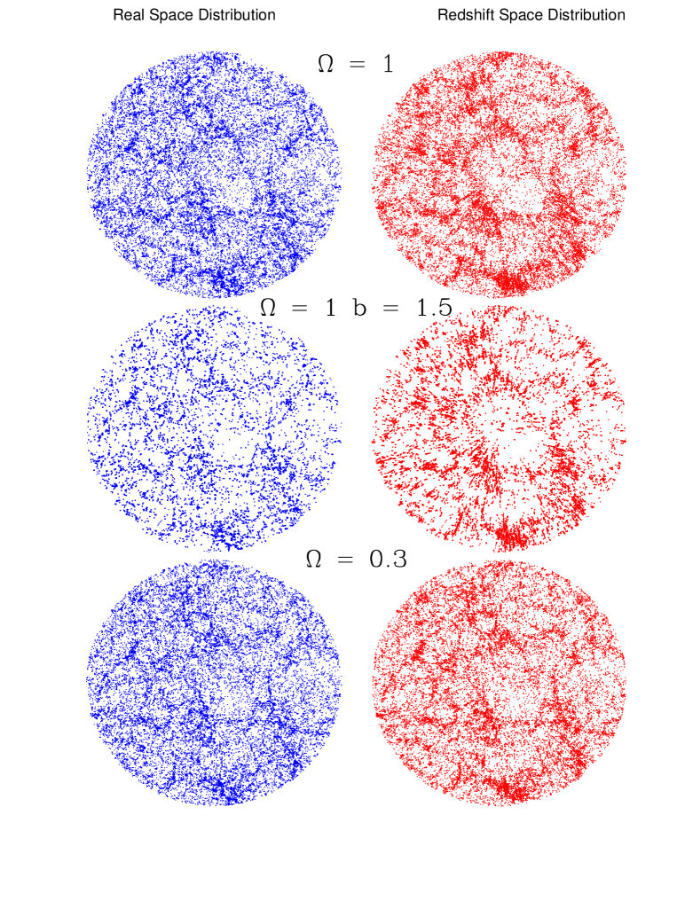
Figure 1: Illustration of redshift distortions for various models

2 Method

According to the Hubble law, $v\simeq cz\simeq H_{0}r$, the recession velocity $v$ of a galaxy, inferred from its redshift, is proportional to its proper distance from the observer, $r$, $H_{0}$ is the Hubble constant today. Irregularities gravitationally generate peculiar velocities ($v_{p}$), so that the true relationship is

$$v=H_{0}r+v_{p}$$ (1)

where $v_{p}$ is the line of sight component of the peculiar motion. Maps of galaxy positions constructed by assuming that velocities are exactly proportional to distance (redshift space) have two principal distortions. The first is generated in dense collapsed structures where there are very many galaxies at essentially the same distance from the observer, each with a random peculiar motion. This results in a radial stretching of the structure known as a “Fingers of God”. The second effect acts on much larger scales (e.g. Kaiser 1987). A large overdensity generates coherent bulk motions in the galaxy distribution as it collapses. Material generally flows towards the center of the structure, i.e. towards the observer for material on the far side of the structure and away from the observer on the near side so it will appear compressed along the line of sight. These effects are large for critical $\Omega_{m}$ and negligible for small $\Omega_{m}$. (For illustration of this effect see http://kusmos.phsx.ukans.edu/ feldman/redshift-distortions.html).

While redshift-space distortions are a nuisance when one wants to construct accurate maps of the (true) spatial distribution of galaxies, they may lead to a robust determination of $\Omega_{m}$ the contribution of clustered matter, (baryonic or not) to the mass density of the Universe.

It has been noticed that superclusters appear to “surround” us, in a preferentially concentric pattern. Although the statistics are poor (few superclusters), it is interesting to ask whether this effect could appear in a homogeneous, isotropic Universe. The effect of peculiar velocity breaks the isotropy in redshift–space diagrams, interacting with inhomogeneities differently depending on how their long axis is oriented.

Our new method is based on the suggestion in Melott et al. (1998); see also Praton et al. (1997). The essence of our method can be explained based on the images in Figure 1 which are slices of 3D simulations. The left side is real–space, the right side redshift–space. The upper row are evolved in a $\Omega_{m}=1$ cosmology ($\lambda=0$), the second row are of a critical CDM cosmology with high bias, the lower an $\Omega_{m}=0.1$ cosmology. All have similar large–scale linear power amplitude and phases at the moment shown. It is clear that the visual concentric effect are much stronger in the high $\Omega$ models in redshift space.

The models we use to illustrate the method have the same initial power spectrum (an $\Omega_{m}=1$ CDM model, normalized to a circle radius of 230 h^-1 Mpc for $h=0.67$ $\sigma_{8}=1$). We use the same spectrum also for the low $\Omega_{m}$ case to make it clear that the effect is rooted in $\Omega_{m}$, not the spectrum. All the slices have very nearly the same number of particles. The effect of peculiar motions is to increase the spacing of large–scale structures in the radial direction as compared with real space, as we show quantitatively below. The enhancement is $\Omega_{m}$–dependent. It is on the basis of this visually–striking difference between the redshift–space behavior of low– and high–density models that we propose a statistic that reproduces the eye’s sensitivity to differences in pattern.

The essence of large–scale redshift space effects is a compression and/or expansion effect along the line of sight. It can best be explained (following Melott et al, 1998) using the Zel’dovich approximation (Zel’dovich 1970) This approximation follows the development of structure by relating the final (Eulerian) position of a particle ${\bf r}$ at some time $t$ to its initial (Lagrangian) position ${\bf q}$ defined at the primordial epoch when particles were smoothly distributed:

$${\bf r}=a(t){\bf x}({\bf q},t)=a(t)[{\bf q}-D_{+}\nabla_{\bf q}\Phi({\bf q})].$$ (2)

In this simple, separable mapping, the displacement field is given by the gradient of the primordial gravitational potential $\Phi$, with respect to the initial coordinates. $a(t)$ is the cosmic scale factor. Differentiating this expression leads to

$${\bf V}={d{\bf r}\over dt}=H{\bf r}-a(t)\dot{D}_{+}\nabla_{\bf q}\Phi({\bf q})$$ (3)

for the velocity of a fluid element ${\bf V}$, where $D_{+}$ is the linear growth of perturbations as a function of time, usually parameterized by $f=d\log D_{+}/d\log a$. This is now known to reproduce weakly non-linear (i.e. large–scale) features in the distribution of matter very accurately indeed, if implemented in an optimized form known as the Truncated Zel’dovich Approximation (Coles et al. 1993, Melott 1994).

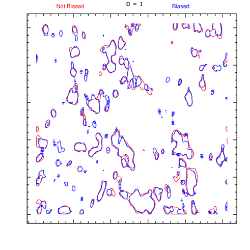
Figure 2: $\Omega=1$ biased (dotted lines) and non–biased (solid) contour levels.

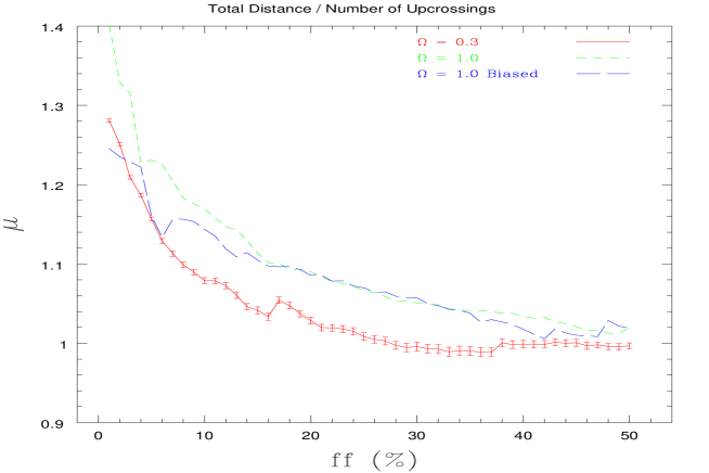
Figure 3: The ratio of parallel to perpendicular distances in a redshift maps. $\mu$ is large for critical $\Omega$ models.

The mapping (3) provides a straightforward explanation of the changed characteristic scale of structures in the redshift direction. Calculating the redshift coordinate exactly and translating it into an effective distance $d_{z}$ gives

$$d_{z}={V\over H}=r_{3}-fa(t)D_{+}(t)\nabla_{3}\Phi({\bf q})=aq_{3}-(1+f)a(t)D_{+}(t)\nabla_{3}\Phi({\bf q}),$$ (4)

in which we have the 3-axis in the redshift direction. Thus the displacement term becomes multiplied by a factor $(1+f)$ in (4) compared to (3). The effect of the displacement field in redshift space is to give the observer a “preview” (albeit in only one direction) of a later stage of the clustering hierarchy. (Note that $\delta$, the density contrast, does not enter here).

We construct density contours for the smoothed field, and take lines-of-sight through the smoothed density field and calculate the rms distance between successive same-direction contour-(up)crossings of high density levels; denoted $S_{\parallel}$. We also do a similar calculation for lines in the direction orthogonal to the observer’s line of sight; denoted $S_{\perp}$ After much experimentation with a large ensemble of simulations, a simple statistic turned out to be nearly optimal; the ratio of the rms spacing in the redshift direction to that in the orthogonal direction, which we call $\mu$:

$$\mu={S_{\parallel}\over S_{\perp}}$$ (5)

In order to examine a density field (the galaxy density in redshift surveys) it is necessary to specify a scale on which the density field will be smoothed. In our case, we want the smoothing scale to include the large–scale dynamics while filtering out small, fully nonlinear dynamics. Then, we must chose one contour level to use for the upcrossing interval measurement.

Although in general contours corresponding to a given filling factor reduce bias dependence, a particular level must be chosen. We choose that level corresponding to filled fraction of 1/8. This fraction has the motivation that dissipationless collapse of a uniform medium will virialize at about this volume fraction. Since with our choice of smoothing we are looking only at just–collapsed structure, this is an appropriate estimate. The use of a small fraction emphasizes the interval between objects, not the size of the objects themselves. We have checked that our measure also has a broad maximum around our choice of filling factor, so that it is not especially sensitive to this choice.

The fundamental object used in this method is the isodensity contour level. Our steps are (1) Make a 2d array consisting of projections of a slice of a 3–D distribution (2) Construct a smoothed density field (3) Make isodensity contour levels corresponding to a set filling factor i.e. fraction of the available area (4) Measure the distance between upcrossings of this contour in the redshift and transverse (real) directions.

To summarize, we show that the typical origin of bias-dependence is absent; we argue that our filling factor approach eliminates another possible source of bias; and we show results of a simulation which behaves in this way (bias insensitive). As can be seen in Figure 2, the bias dependence is negligible since the contours change little in the biased model.

In figure 3 we show the results of the simulations. We plot $\mu$ (see 5) vs filling factor ($ff$). we added the error bars only to one line, but they are of similar magnitude. We see that the critical $\Omega$ models behave similarly and are significantly different than the low ($\Omega=0.3$) model.

3 Conclusions

In the next few years, astronomers will map an appreciable fraction of the Universe by redshift surveys where recession speed is assumed to be proportional to distance. Gravity induce peculiar motions of galaxies as part of the ongoing process of structure formation. We showed that such motions tend to enhance redshift structures concentric about the observer, and argued that the strength of this effect may be a powerful new probe of the mass density of the Universe.

The principal limitations of this method are the following:

• The smoothing length is specified by the autocorrelation function. Biasing may affect this somewhat (small effect).

• The spacing ratio $\mu\neq 1$ for low $\Omega$ models. This is due to the fact that the “fingers of God” effect introduce noise (small effect).

• The method requires deep, dense, 3–D redshift surveys where the correlation length is much smaller than the survey effective radius. These surveys are coming (SDSS, 2DF)

• The method measures $\Omega_{m}$ not $\Lambda$.

The advantages of this method are:

• No need for distance measurements, redshifts are enough.

• No comparison between the density field and the velocity field. Thus we measure $\Omega$ directly no $\beta=\Omega^{0.6}/b$, that is, virtually no bias dependence.

• Bias affects this statistic only through excess smoothing which is both a weak effect and can be controlled easily.

- [1] oles P., Melott A.L., & Shandarin S.F. 1993, MNRAS, 260, 765
- [2] aiser, N. 1987, MNRAS, 260, 705
- [3] elott A.L. 1994, ApJ, 426, L19
- [4] elott A.L., Coles, P., Feldman, H. and Wilhite, B. 1998, ApJ496, L85
- [5] eebles P.J.E., 1980. The Large–scale Structure of the Universe (Princeton University Press, Princeton)
- [6] raton E.A., Melott A.L., & McKee M.Q. 1997, ApJ, 479, L15
- [7] el’dovich Ya.B. 1970, A&A, 5, 84