What can we learn from the fluxes of the 1.2 Jy IRAS sample?

Abstract

We present a new method for fitting peculiar velocity models to complete flux limited magnitude-redshifts catalogues, using the luminosity function of the sources as a distance indicator. The method is characterized by its robustness. In particular, no assumptions are made concerning the spatial distribution of sources and their luminosity function. Moreover the inclusion of additional observables, such for example the one carrying the Tully-Fisher information, is straightforward.
As an illustration of the method, the predicted IRAS peculiar velocity model is herein tested using the fluxes of the IRAS 1.2 Jy sample as the distance indicator. The results suggest that this model, while successful in reproducing locally the cosmic flow, fails to describe the kinematics on larger scales.

1 The method

The application of the method is restricted to samples strictly complete up to a given magnitude limit $m_{\rm lim}$, i.e. the selection function in apparent magnitude is well described by a sharp cut-off $\psi(m)=\theta(m_{\rm lim}-m)$ with $\theta(x)$ the Heaveside function. The probability density of the sample may be written in this case as

$$dP=\frac{1}{A}h(\mu,l,b)\cos b\,dldbd\mu\,f(M)dM\,\theta(m_{\rm lim}-m)$$ (1)

where $\mu=m-M$ is the distance modulus, $h(\mu,l,b)$ the line-of-sight distribution function, $f(M)$ the luminosity function and $A$ is the normalisation factor warranting $\int dP=1$.

The milestone of the method consists in defining the random variable $\zeta$ as follows

$$\zeta=\frac{F(M)}{F(M_{\rm lim})}\,\,\,\,\,\,\,\,\,\,\,\,\,\,;\,\,\,\,\,\,\,\,\,\,\,\,\,\,d\zeta=\frac{f(M)}{F(M_{\rm lim})}\,dM$$ (2)

where $F(M)=\int_{-\infty}^{M}f(x)dx$ stands for the cumulative distribution function in $M$ and $M_{\rm lim}\equiv M_{\rm lim}(\mu)$ is the maximum absolute magnitude for which a galaxy at distance $\mu$ would be visible in the sample (e.g. $M_{\rm lim}(\mu)=m_{\rm lim}-\mu$ if the k-correction is neglected). By definition, the random variable $\zeta$ for a sampled galaxy belongs to the interval $[0,1]$. The probability density of Eq. (1) reduces to

$$dP=\frac{1}{A}h(\mu,l,b)\,F(M_{\rm lim}(\mu))\,\cos b\,dldbd\mu\,\times\,\theta(\zeta)\,\theta(1-\zeta)\,d\zeta$$ (3)

This equation implies the two following properties:

• P1: $\zeta$ is uniformly distributed between $0$ and $1$.

• P2: $\zeta$ and $\mu$ are statistically independent, i.e. the distribution of $\zeta$ does not depend on the spatial position of the galaxies.

The random variable $\zeta$ can be estimated without any prior knowledge of the cumulative luminosity function $F(M)$. For each galaxy $(M_{i},\mu_{i})$ one can indeed form the subsample $S_{i}=S_{1}\cup S_{2}$ with $S_{1}=\{\,(M,\mu){\rm~{}such~{}that~{}}M\leq M_{i}{\rm~{}and~{}}\mu\leq\mu_{i}\,\}$ and $S_{2}=\{\,(M,\mu){\rm~{}such~{}that~{}}M_{i}<M\leq M^{i}_{\rm lim}{\rm~{}and~{}}\mu\leq\mu_{i}\,\}$. By construction (see figure 1) $M$ and $\mu$ are independent in each subsample $S_{i}$. This implies that the following quantity is an unbiased estimate of the random variable $\zeta$

$${\hat{\zeta}_{i}}=\frac{r_{i}}{n_{i}+1}$$ (4)

where $n_{i}$ is the number of objects in $S_{i}=S_{1}\cup S_{2}$ and $r_{i}$ the number of objects in $S_{1}$ (see Efron & Petrosian 1992).

The radial peculiar velocity field is herein described by a linear model parametrized by a $N$-dimensional vector ${\bf\beta}=(\beta_{1},\beta_{2},...,\beta_{N})$,

$$v_{\bf\beta}\equiv v_{\bf\beta}({\bf r})=\sum_{k=1}^{N}\beta_{k}\,v_{k}({\bf r})$$ (5)

where $v_{1}({\bf r})$, $v_{2}({\bf r})$, …, $v_{N}({\bf r})$ is a set of functions depending on the spatial position ${\bf r}$. It assumed hereafter that there exists a solution ${\bf\beta}^{\star}$ fairly reproducing the true radial peculiar velocities of galaxies $v_{i}\equiv v({\bf r}_{i})\simeq v_{{\bf\beta}^{\star}}({\bf r}_{i})$. For a given vector ${\bf\beta}$, the model dependent variables $\mu_{\bf\beta}$ and $M_{\bf\beta}$ can be computed from the observed redshift $z$ and apparent magnitude $m$ following

$$\mu_{\bf\beta}=5\,\log_{10}\frac{cz}{H_{0}}+25-u_{\bf\beta}\,\,\,\,;\,\,\,\,M_{\bf\beta}=m-\mu_{\bf\beta}\,\,\,\,;\,\,\,\,u_{\bf\beta}=-5\,\log_{10}\left(1-\frac{v_{\bf\beta}}{cz}\right)$$ (6)

The quantities $\mu_{\bf\beta}$ and $M_{\bf\beta}$ are related to the true absolute magnitude $M$ and distance modulus $\mu$ via $\mu_{\bf\beta}=\mu+u_{\bf\beta^{\star}}-u_{\bf\beta}$ and $M_{\bf\beta}=M-u_{\bf\beta^{\star}}+u_{\bf\beta}$.

It is shown in Rauzy&Hendry (hereafter RH) that any test of independence between $\zeta_{\beta}$ computed following Eq. (4) and $u_{\beta}$ provides us with an unbiased estimate of $\beta^{\star}$. In particular the coefficient of correlation $\rho(\zeta_{\beta},u_{\beta})$ has to vanish when $\beta={\beta^{\star}}$, i.e.

$$\beta={\beta^{\star}}\,\,\,\,\,\Longleftrightarrow\,\,\,\,\,\rho(\zeta_{\beta},u_{\beta})=0$$ (7)

The accuracy of this estimator can be obtained through numerical simulations by analysing the influence of sampling fluctuations on the coefficient of correlation.

This estimator is clearly robust. Nothing has been assumed concerning the spatial distribution of sources nor on the shape of their luminosity function. In particular the method is free of Malmquist-like biases. Moreover the inclusion of a second observable parameter, for example in order to account for Tully-Fisher information, can be achieved without any difficulty. Finally it is worthwhile to mention that the method will benefit from the use of the velocity orthogonalization procedure proposed by Nusser & Davis (1995) (see RH for details).

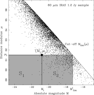
Figure 1: Distance modulus versus absolute magnitude for the 60 $\mu$m IRAS 1.2 Jy sample (5321 galaxies)

2 Application to the IRAS 1.2 Jy sample

The method is herein applied to the 60 $\mu$m IRAS 1.2 Jy sample (Fisher et al. 1995). The distance modulus versus absolute magnitude diagram is shown in figure 1. The peculiar velocity field model tested is the predicted IRAS velocity field (Strauss et al. 1992) characterized by only one parameter $\beta=\Omega_{0.6}/b_{I}$. The luminosity function of these sources does not exhibit any turnover towards the faint-end tail, at least within the observed range of magnitudes. Due to the large spread of the LF, one cannot expect very high constraints on the velocity model tested. However a rejection test for the $\beta$ parameter can be constructed. We obtained that $\beta\geq 0.7$ can be rejected with a confidence level of 95% and $\beta\geq 1.1$ with a confidence level of 99%.

In a second step, we use the observed correlation between the absolute magnitude $M$ and some ”colour index” defined as $p=2.5\log_{10}(F_{100}/F_{60})$ (with $F_{100}$ the flux at 100 $\mu$m) in order to refine the analysis. The data have been grouped in $8$ classes by interval of $p$. Because of the correlation between $p$ and $M$, the spread of the luminosity function for each of these classes taken individually is expected to be smaller than the spread of the global luminosity function, and thus the accuracy of the distance indicator improved. The random variable $\zeta_{\beta}$ is then computed using Eq. (4) but this time class by class. The correlation between $\zeta_{\beta}$ and the velocity modulus $u_{\beta}$ is after that evaluated for the whole sample.

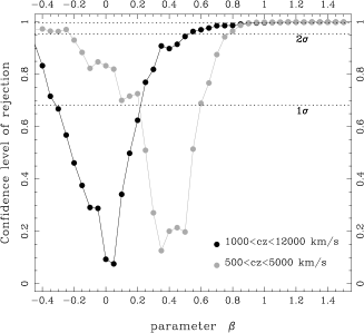
Figure 2: Confidence level of rejection for the parameter $\beta$

The results are presented in figure 2 in terms of the confidence level of rejection for the parameter $\beta$. The method has been first applied to the galaxies within the redshift range 1000-12000 km s^-1. It is found that $\beta\in[-0.35,0.25]$ at $1\sigma$, and that models with $\beta\geq 0.5$ can be rejected with a confidence level of 95%. This result is in disagreement with most of the analyses based on Tully-Fisher data (e.g. VELMOD on MarkIII (Willick & Strauss 1998), ITF method on SFI (Da Costa et al. 1998) favoring a value of $\beta=0.5$. We interpret this discrepancy as follows.

When fitting a velocity model to data, the natural weight assigned by the fitting procedure to each galaxy is roughly proportional to the inverse of its redshift. The mean effective depth of the volume where the velocity model is compared to data has to be estimated using these weights. For our first sample with $z\in[1000,12000]$ km s^-1, we find a mean effective depth $3800$ km s^-1. In order to mimic the effective volume sampled by Tully-Fisher data we have applied the method to a truncated version of the IRAS sample containing 1621 galaxies with $z\in[500,5000]$ and galactic latitude $|b|>20$ (the mean effective depth of this sample is 2200 km s^-1). Figure 2 shows that the value of $\beta$ estimated from this truncated sample is fully consistent with the values obtained using Tully-Fisher data. An interpretation of these results could be that the predicted IRAS velocity field model, while successful in reproducing locally the cosmic flow, fails to describe the kinematics on larger scales.

- [1] a Costa L.N., Nusser A., Freudling W., Giovanelli R., Haynes M.P., Salzer J.J., Wegner G. 1998, MNRAS 229, 425
- [2] fron B., Petrosian V. 1992, ApJ 399, 345
- [3] isher K.B.,Huchra J.P., Strauss M.A., Davis M., Yahil A., Schlegel D. 1995, ApJS 100, 69
- [4] usser A., Davis M. 1995, MNRAS 276, 1391
- [5] auzy S., Hendry M.A. 1999, in preparation
- [6] trauss M.A., Davis M., Yahil A.,Huchra J.P. 1992, ApJ 385, 421
- [7] illick J.A., Strauss M.A. 1998, ApJ 507, 64
- [8]