Simulations of Nonthermal Electron Transport in Multidimensional Flows: Synthetic Observations of Radio Galaxies

Abstract

We have applied an effective numerical scheme for cosmic-ray transport to 3D MHD simulations of jet flow in radio galaxies (see the companion paper by Jones et al. 1999). The marriage of relativistic particle and 3D magnetic field information allows us to construct a rich set of “synthetic observations” of our simulated objects. The information is sufficient to calculate the “true” synchrotron emissivity at a given frequency using explicit information about the relativistic electrons. This enables us to produce synchrotron surface-brightness maps, including polarization. Inverse-Compton X-ray surface-brightness maps may also be produced. First results intended to explore the connection between jet dynamics and electron transport in radio lobes are discussed. We infer lobe magnetic field values by comparison of synthetically observed X-ray and synchrotron fluxes, and find these “inverse-Compton” fields to be quite consistent with the actual RMS field averaged over the lobe. The simplest minimum energy calculation from the synthetic observations also seems to agree with the actual simulated source properties.

, , ,

1 Introduction

Numerical simulations of extragalactic jets have been used for well over a decade to shed light on the physical processes taking place within radio galaxies. There is an important and sometimes overlooked issue when making the comparison between numerical simulations and observed sources: the link between dynamical processes and the resulting emissions. Synthetic observations can address this issue. By synthetically observing a source whose detailed physical structure is known beforehand, we can gain insights into what real observations are actually telling us.

Attempts have been made to obtain emission characteristics from purely hydrodynamical simulations. The earliest versions estimated the local magnetic field strength by assuming it to be proportional to the density, providing a means to derive a crude synchrotron “pseudoemissivity.” ? made comparisons between observed hot spot morphologies and simulated hot spot dynamics in this way. Yet purely hydrodynamical simulations can never truly model the jet synchrotron emission, as emphasized by ?, who found that the distribution of hydrodynamic variables provides little insight into the observed intensity distribution in relativistic hydrodynamic simulations. Inclusion of even a passive vector magnetic field (e.g., Laing 1981; Clarke, Norman, & Burns 1989) seemed to offer a big step forward, since the synchrotron emission reflects in part the magnetic field distribution, and since it allows one to calculate observable polarization properties. At this level synthetic synchrotron brightness distributions show encouraging morphological similarities to real radio galaxies.

However, synthetic radio observations from large-scale, fully 3-dimensional purely magnetohydrodynamical simulations still require critical arbitrary assumptions to model the emission. In addition, the emission spectrum cannot be obtained this way (?). Only an explicit treatment of the relativistic electron population can allow us to treat the emission properties of the simulation directly. Jones, Ryu & Engel (1999) (JRE99) and Jones, Tregillis & Ryu (these proceedings) (JTR99) describe a computationally economical technique for relativistic particle transport within multidimensional MHD flows. This scheme can follow explicitly diffusive acceleration at shocks and second-order Fermi acceleration in smooth flows. It also accounts for adiabatic losses, synchrotron and inverse-Compton losses, and injection of fresh particles at shocks.

We have begun a series of 3-dimensional MHD simulations of extragalactic radio jets utilizing this nonthermal particle transport scheme. From the data produced by these radio galaxy simulations we can conduct a very rich set of synthetic observations, because for the first time we are able to compute in each source volume element the number of relativistic electrons at the energy radiating at a chosen frequency. Presented here are some results from our first suite of synthetic observations, which demonstrate the kinds of insights that can be obtained from this tool. Related dynamical aspects of the simulations are described in JTR99.

2 Synthetic Observation Methods

The combination of a vector magnetic field structure and a nonthermal particle energy distribution makes it possible for us to compute an approximate synchrotron emissivity, complete with spectral and polarization information, in every zone of the computational grid. Surface-brightness maps for the optically-thin emission are then easily produced by ray tracing through the computational grid, thereby projecting the source onto the plane of the sky. We have also produced X-ray surface brightness maps in the same fashion, by calculating the inverse-Compton (IC) emissivity from the interaction between the cosmic microwave background radiation and our nonthermal electrons. Future work will include a more sophisticated treatment of the X-ray emission, including synchrotron and AGN seed photons.

The synthetic observations can be imported into any standard image analysis package and analyzed like actual observations. To make this exercise as realistic as possible we place the simulated object at an appropriate distance, currently 100 Mpc, and then convolve the computed surface brightness distribution with typically sized Gaussian beams. We can then explore a range of observable properties at multiple wavelengths, multiple angular resolutions and so on. The real power in this method comes from the fact that we can then compare synthetically “observed” source properties with the actual physical properties of the simulated objects. We can, for instance, extract the true magnetic field strength and topology in a particular region, particle and field “filling factors”, or the distributions of particle spectral forms in an emitting volume.

3 Discussion

Figure 1 illustrates “observed” radio synchrotron and X-ray IC images constructed in this way from a 3-dimensional simulation described in JTR99. Briefly, it represents emission from a light, supersonic jet, with density $10^{-2}$ of the ambient medium, and internal Mach number of 8. For the other parameters mentioned below this corresponds to a jet velocity of $0.1c$. The jet inflow slowly precesses around a cone of opening angle $5^{o}$, to break cylindrical symmetry. The incoming jet core radius was $r_{j}=1$ kpc, and the magnetic field on the jet axis was $B_{0}=1\mu$G, with a gas pressure there 100 times greater than the magnetic pressure. This leads to a jet kinetic power of $\approx 10^{37}$ W. For this simulation a relativistic electron population with a power law momentum index, $f(p)\propto p^{-4.4}$ (corresponding to a synchrotron spectral index $\alpha=0.7$) was brought onto the grid with the jet flow. That population was subjected to acceleration at shocks, adiabatic and radiative losses. No additional nonthermal electrons were injected at shocks, however. In this simulation, the synchrotron cooling time for $\gamma=10^{4}$ electrons radiating on the jet axis ($\nu\sim 300$ MHz) is $3.7\times 10^{8}$ years, whereas the analogous inverse-Compton ($h\nu\sim 100$ keV) cooling time is $4.7\times 10^{7}$ years. The synthetic observations presented here correspond to a time when the jet has propagated approximately $10^{6}$ years, rendering these cooling effects negligible. The 1.4 GHz synchrotron luminosity $\nu L_{\nu}$ is $5.3\times 10^{32}\times\delta_{4}$ W, where $\delta_{4}=10^{4}\delta$, and $\delta$ is the ratio of nonthermal to thermal electron densities at the jet orifice.

In what follows we have set $\delta_{4}=1$, motivated by estimates of injection efficiencies at nonrelativistic shocks (e.g., ?). It gives the simulated synchrotron source a relatively low luminosity compared to typical FR2 objects. It guarantees, however, that the relativistic electrons are passive. In fact, the integrated pressure in relativistic electrons ($E>mc^{2}$) is everywhere less than 0.1% of the thermal pressure. Given that, the synthetic observations can all be scaled simply in terms of $\delta$, or in some cases, are independent of $\delta$. If, for comparison, we assume from the same motivations that cosmic-ray ions have $\sim 100$ times more energy than electrons, those nonthermal ions could locally contribute up to $\sim 10$% of the total pressure. With these assumptions our simulated source is out of equipartition between relativistic particles and magnetic fields, with the balance in favor of particles.

The synchrotron synthetic observation in Figure 1 corresponds to a frequency of 1.4 GHz, and the X-ray image to an energy of 10 keV. With the source distance assumed to be 100 Mpc the synchrotron flux over the source is about $330\times\delta_{4}$ mJy. The 10 keV inverse-Compton flux is $2.4\times 10^{-10}\times\delta_{4}$ Jy corresponding to a 10 keV luminosity $\nu L_{\nu}$ of $6.5\times 10^{32}\times\delta_{4}$ W.

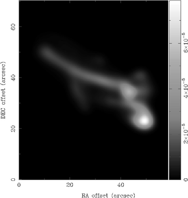
Figure 1: Synthetic surface brightness maps constructed as described in the text and analyzed with the MIRIAD package. The left panel is 1.4GHz synchrotron emission; the right panel is 10keV inverse-Compton X-ray emission. The linearly-scaled colorbar values represent Janskys per 3.5” beam.

In the images one can clearly separate the jet, a terminal hot spot, a secondary hot spot and the diffuse lobe. The contrast in the radio image between the jet core and the outer lobe is higher than sometimes observed in real sources. There are two primary reasons why the jet is so prominent. First, the entire cosmic-ray electron population passes down the jet in this simulation, so the density of relativistic electrons is higher there than anyplace else. (See the 2-dimensional simulations of JRE99 to measure the importance of this modeling choice.) Since the magnetic field is stronger inside the jet than in much of the lobe volume, the synchrotron emissivity is relatively large there. In addition, the source in Figure 1 is quite young dynamically, so that a line of sight path length through the jet is roughly 20% of the path through the lobe. As this source aged that comparison would change significantly in favor of the lobe path length, of course.

While there is an overall correspondence between the radio and X-ray images, there are some significant differences. The jet/lobe and hot-spot/lobe contrasts are much more pronounced in the synchrotron map. Calculating the average surface brightness in the jets and in the lobes of the two maps, we find that this ratio is about three times higher in the radio map than in the X-ray map. While the radio hot spots do appear to have X-ray bright counterparts, there are also bright X-ray regions without corresponding radio enhancements. The inverse-Compton emission arises from a particle population of fixed energy ($\sim 1$ GeV at 10 keV), while the synchrotron emission at fixed frequency does not. Thus, the surface brightness of IC emission from the CMB simply reflects the column density of electrons in a fixed energy range, while the synchrotron is biased to regions where the fields are strongest, both because radiative power is greater there, but also because one sees emission from relatively more plentiful lower energy electrons. In cases where radiative losses are significant in the GeV range so that the spectra steepen, these differences would become even more dramatic.

Comparison of the two prominent hot spots reveals some interesting contrasts. The larger primary hot spot at the right edge of the radio lobe corresponds to an extremely complicated set of structures near the jet terminus. While it is nominally associated with the end of the jet flow, the jet terminal shock is very small and influences the spectrum of only a tiny portion of the electrons in the hot spot. In fact, much of the emergent jet flow has not passed through any strong shock before reaching the cocoon. Some of the electron population shows signs of significant shock acceleration, but the pattern is not simple (see also JTR99.) Over all, the influence of shock acceleration on the brightness and spectrum of the primary hot spot is quite small. The enhanced emission is mostly due to magnetic field amplification in the complex flows there rather than particle acceleration.

On the other hand, there is clear evidence for particle acceleration in the secondary hot spot further back in the lobe, which has a much different character. This hot spot has a distinctly flatter spectrum ($\alpha\approx 0.6$) than the jet ($\alpha=0.7$). The surface brightness map would make it appear that the jet flows directly into this hot spot. However, this is an accident of projection. The high emissivity volume really is well outside the jet, and examination of the plasma streak lines reveals that this hot spot actually corresponds to flow downstream of a moderately strong shock formed in the cocoon “backflow”, as discussed in JTR99.

One of the greatest potential applications of synthetic observations is comparisons between the real physical properties of a simulated object and observationally inferred source properties, which are generally based on convenient, simplified assumptions. Here we provide a couple of preliminary examples, from the simulation described above and in JTR99. From comparison of the integrated radio synchrotron and X-ray IC measured fluxes, we can infer a magnetic field within the source (e.g., ?). For our simulated source and synthesized observations the resulting “inverse-Compton” field is

$B_{ic}=1.0~{}\mu{\rm G}$,

which matches very well the actual volume-averaged RMS field within the lobes; namely, $B_{rms}=1.2~{}\mu$G. That is a very encouraging result, especially since the magnetic field in the source is really quite filamentary, with an “intermittency” ($\left<B^{4}\right>/(\left<B^{2}\right>^{2})\approx 5.7$ at the time shown. The maximum field value in the lobes is $12~{}\mu$G and the minimum field value is $0.003~{}\mu$G.

We also can apply standard minimum-energy arguments (between nonthermal particles and magnetic fields) to the observed synchrotron flux for an associated magnetic field strength. Again integrating over the source, this gives (e.g., ?)

$B_{me}=(5.4~{}\mu{\rm G})\times((1+k)/(101\eta))^{2/7}\times\delta_{4}^{2/7}$,

where $\eta$ is the filling factor and $k$ is the ratio of nonthermal ion to electron energies. Even with $\eta=1$ this minimum energy magnetic field value exceeds the actual RMS field and the IC estimate by roughly a factor of 5, warning us that the field is not in a minimum-energy configuration. More realistic choices for the filling factor would increase that difference. This result is very consistent with the actual simulated source properties, because, as noted earlier, with $\delta_{4}=1$ and $k=100$, nonthermal particle energies do actually exceed the global magnetic field energy by an order of magnitude or more. Thus, again, we find this an optimistic result, because it suggests the combined use of IC and minimum energy magnetic field estimates may be able to give us reliable information about the actual fields and the actual partitioning of energy between particles and fields.

This work was supported at the University of Minnesota by the NSF through grant AST96-16964 and by the University of Minnesota Supercomputing Institute. DR was supported in part by KOSEF through grant 981-0203-011-02.

References

- [1]
- [2] [] Clarke, D. A., Norman, M. L., and Burns, J. O. 1989, ApJ, 342, 700.
- [3]
- [4] [] Clarke, D. A., 1993, in: Proceedings of the Ringberg Workshop on “Jets in Extragalactic Radio Sources”, eds. H.-J. Roser, K. Meisenheimer, (Springer Verlag, Berlin), p. 243.
- [5]
- [6] [] Feigelson, E. D., Laurant-Muehleisen, S. A., Kollgaard, R. I., and Fomalont, E. B. 1995, ApJ, 449, L149.
- [7]
- [8] [] Harris, D. E., and Grindlay, J. E. 1979, MNRAS, 188, 25.
- [9]
- [10] [] Hughes, Phillip, Duncan, Comer, and Mioduszewski, Amy, 1996, in: Energy Transport in Radio Galaxies and Quasars, eds. P.E. Hardee, A.H. Bridle, J.A. Zensus (Astronomical Society of the Pacific, San Francisco), p. 137.
- [11]
- [12] [] Jones, T. W., Ryu, D., and Engel, A. 1999, ApJ, 512, 105.
- [13]
- [14] [] Jones, T. W., Tregillis, I. L., and Ryu, D. 1999 (these proceedings).
- [15]
- [16] [] Laing, R. A. 1981, ApJ, 248, 87.
- [17]
- [18] [] Smith, M. D., Norman, M. L., Winkler, A. K.-H., and Smarr, L. 1985, MNRAS, 214, 67.
- [19]