Multi-frequency observations as a key to source and environment parameters of FRII objects

Abstract

Our knowledge of the environments of radio-loud AGN is still sketchy. However, to understand the jet phenomenon it is important to know about the properties of the surroundings in which jets are formed and evolve. Here I present an analytical model of the radio surface brightness distribution of the large scale structure of FRII-type radio sources. The ‘virtual maps’ resulting from this model can be compared with observed maps to obtain estimates for a range of source properties from the model. These properties include parameters describing the gas density distribution of the source environment, the energy transport rate of the jets and the orientation angle of the source jet axis with respect to the line of sight. The model is tested using radio maps of Cygnus A for which there are independent measurements of some of these parameters available in the literature. The model estimates agree well with these observations. Varying the resolution of the radio maps used in the comparison does not change the results significantly.

1 Introduction

The properties of AGN and their environments are of crucial importance for many aspects of astrophysics. In the early universe the space density of AGNs was orders of magnitude greater than it is today dp90,hs90e.g.. At the same time evidence is accumulating that AGNs at high redshift, at least those which are radio-loud, reside in the most massive and most evolved systems of the respective epoch blr98e.g.. It is therefore of great importance for models of structure formation in the universe to know the properties of the environments of radio sources.

The jets in powerful radio galaxies and radio-loud quasars are presumably powered by accretion discs around supermassive black holes. This general picture is well accepted (however, see Kundt, this volume) but the details of exactly how the jet material is accelerated are still not very well understood. In this respect it is important to know how much energy is transported along the jets because this places constraints on the efficiency with which energy is channeled from the accretion disc into the jet flow.

The hot, gaseous environments of radio sources can be observed directly at X-ray frequencies. The temperature of this gas and its density can be derived from this emission. Unfortunately, the limited sensitivity and resolution of X-ray telescopes confines this method to objects at low to, at best, intermediate redshifts (see Worrall, this volume). The uncertainties introduced by the additional X-ray emission from the AGN itself are increased further by the possible scattering of some of the X-rays emitted by the AGN off the material in the environment of the source [bcsf99]. Also, the large scale radio structure embedded in the hot gas modifies the X-ray emission properties of this material [ka99].

Optical emission from the surroundings of the large scale structure of radio galaxies is detected in some objects on scales $\leq 100$ kpc and is often found to be aligned with the radio source at redshifts beyond $z\sim 0.6$ pm93e.g.. If the flux of ionising photons from the AGN is known in these objects, then it is possible to determine the density of the emitting material. However, the optical light is emitted by the warm phase ($\sim 10^{4}$ K) rather than the hot phase ($\sim 10^{7}$ K) of the gas in the surroundings of radio sources. The inferred volume filling factors of the warm phase are small and so the properties of the bulk of the gas, which is hot, cannot be determined from the optical emission. Additionally, the properties of the warm gas phase may also be changed by the expansion of the large scale structure of the radio source [ksr99].

The radio emission of the large scale structure itself may also be used in the determination of the properties of the environment. The material external to the radio lobes is modifying the polarisation properties of this radiation via Faraday rotation. The Rotation Measure (RM) can be used to infer the density of the material creating this Faraday screen. However, the RM depends not only on the gas density but also on the strength of the magnetic field within this material which is usually not very well constrained. The Faraday screen is also known to be far from uniform. It is spatially correlated with the optical emission in some sources and the RM may therefore also probe predominantly the warm gas phase rather then the hot phase [cmb90].

Constraining the jet power, i.e. the energy transport rate of the jets, from radio observations usually involves some estimate of the total energy content of the large scale structure and of the age of the source in question. In most cases it is assumed that the population of relativistic electrons is uniformly distributed over the radio lobes and aging of the initial population is neglected in the energy estimates. Spectral index maps, which are sometimes used for the same sources to estimate their spectral ages, clearly demonstrate that this is a poor assumption. Furthermore, in almost all sources the orientation of the radio structure to the line of sight is unknown which leads to errors in the estimation of the volume occupied by the radio plasma. On the other hand multifrequency radio observations are available for many radio sources of type FRII at all redshifts. Using these maps to determine the properties of the radio sources and their environments would provide a wealth of information without the need of additional extensive observational programmes in many different wavebands.

In the following I will therefore present a model which attempts to determine the properties of the jets and those of the environment of FRII sources using only radio maps at two observing frequencies. The model predicts the radio surface brightness distribution of the large scale structure of FRII-type objects based on 8 model parameters. These parameters include the energy transport rate of the jets, the gas density distribution of the source environment and the angle of the jet axis with the line of sight. These ‘virtual radio maps’ are then compared to observations and the best fitting model parameters are found. To determine the quality of these estimates I use radio maps of Cygnus A for which independent measurements of some of these quantities exist in the literature.

2 The model

2.1 The dynamical evolution of FRII sources

The model presented here is based on a model for the dynamics of FRII-type radio sources developed in Kaiser & Alexander (1997). The basic features of this model can be summarised as follows. The usual geometry of jets embedded in a cocoon which in turn is surrounded by a bow shock as proposed by Scheuer (1974) is assumed. Parts of the cocoon are identified as the observable radio lobes. The jets are assumed to be in pressure equilibrium with the cocoon. Because of the high sound speed in this region, the pressure within the cocoon should be constant [ka97] away from the region right next to the hot spots which implies that the radius of the jets should remain constant throughout the cocoon. The forward expansion of the cocoon is balanced by the ram pressure of the surrounding gas which is pushed aside. The model does not involve an assumption concerning the expansion of the cocoon perpendicular to the jet axis. This implies that the model results are independent of the exact geometrical shape of the cocoon. The gas density of the external medium the source is expanding into is modeled with a power law:

$$\rho=\rho_{o}\left(r/a_{o}\right)^{-\beta},$$ (1)

where $r$ is the radial distance from the centre of the distribution. Note, that the external density is therefore described by two parameters, the exponent of the power law $\beta$ and the combination $\rho_{o}a_{o}^{\beta}$ of the central density, $\rho_{o}$, and the core radius, $a_{o}$. This model then predicts the expansion of the cocoon to be self-similar which is supported by observations [lw84, lms89].

2.2 Radio emission of the cocoon

The radio synchrotron emission of the cocoon is radiated by relativistic electrons and may be also positrons gyrating about the magnetic field lines within the cocoon. The spectral distribution of the radiation emitted by a given electron depends on its energy. The energy of a given electron is constantly changing because of losses due to the (approximately) adiabatic expansion of the cocoon, synchrotron radiation itself and inverse Compton scattering of the cosmic microwave background photons. Of course the relativistic electrons may gain energy as well if efficient reacceleration processes are at work within the cocoon. For simplicity it is assumed in the following that the relativistic particles are only accelerated once at the termination shock of the jet.

All of the processes that may change the evolution of the energy spectrum of the radiating relativistic particles are time dependent. They will therefore have changed this spectrum to a larger extent in parts of the cocoon which were injected by the jets at earlier times. To keep track of these changes it is necessary to split the cocoon into smaller volume elements characterised by their injection time, $t_{i}$, into the cocoon. The evolution of the energy spectrum of relativistic particles within each element is then followed separately. This technique is described in greater detail in Kaiser, Dennett-Thorpe & Alexander (1997).

To proceed it is assumed that the energy spectrum of the relativistic particles is initially given by a power law, $n\propto\gamma^{-p}$, where $\gamma$ is the relativistic Lorentz factor. The spectrum is cut-off at high energies corresponding to $\gamma_{max}$. The model then allows to calculate the synchrotron emissivity of the volume elements for a given source age. Summing contributions of all the elements then yields the total luminosity of the cocoon of the source.

2.3 Spatial distribution of the radio emission

The volume elements that are employed to follow the evolution of the energy spectrum of the relativistic particles are ‘labeled’ with their injection time, $t_{i}$, but their spatial positions within the cocoon are not specified. Therefore no assumption has been made so far concerning the geometrical shape of the cocoon and it is possible to choose a functional form for the surface delineating the cocoon boundary which satisfies the shape of observed radio lobes. Assuming rotational symmetry about the jet axis the parameterisation

$$y=Lb_{o}\left(1-l_{x}^{2}\right)^{b_{1}},$$ (2)

in the plane containing the jet axis completely determines the cocoon surface. Here $l_{x}$ is the dimensionless coordinate $l_{x}=x/L$ (see Figure 1) with $L$ being the length of one jet. The parameters $b_{o}$ and $b_{1}$ determine the aspect ratio of the cocoon and the ‘bluntness’ of its leading edge respectively.

Figure 1: The geometry of the cocoon.

In order to follow the evolution of the volume elements introduced above not only in time but also in space, I now make the very simplistic assumption that these elements can be identified with thin cylindrical slices which are rotationally symmetric about the jet axis (see Figure 1). This set-up was originally proposed by Chyży (1997) and has several implications. Firstly, the contents of two neighboring slices are not allowed to mix. This assumption is certainly too simplistic but because of the absence of pressure gradients within the cocoon, which was assumed earlier, mixing of thermal material and tangled magnetic field does not significantly change the relevant conditions within the cocoon. Next, the possible diffusion of relativistic particles does not significantly change their energy distribution locally. This may hold, at least to some extent, because the charged particles are tied to the magnetic field lines which are assumed to be tangled on scales small compared to the dimensions of the cocoon. Also the stochastic nature of the diffusion process precludes the accumulation of relativistic particles of a small energy range within a small volume and their depletion in the rest of the cocoon. Finally, the individual slices must move as rigid entities, i.e. the centre of a slice does not overtake its edge or vice versa. Given these caveats, plus the assumption that there is no significant reacceleration of relativistic particles in the cocoon, it is probably best to view this model as describing the average conditions within the cocoon at the position of a given slice.

The dynamical evolution underlying this emission model is self-similar which implies for this model that all physical quantities behave as power laws of age of the radio source. The dimensionless position of a slice or volume element injected by the jet into the cocoon at time $t_{i}$ is therefore set to $l_{x}=x/L\equiv(t_{i}/t)^{a}$. The value of $a$ is determined by the requirement that the sum of all volume elements must be equal to the total volume of the cocoon.

Using this model it is now possible to create surface brightness plots of FRII radio sources for a given set of source and environment parameters by integrating the emissivity along the lines of sight through the cocoon. To compare the model predictions with observations the angle of the jet axis to the line of sight must also be specified. In total there are 8 parameters in this model which determine the predicted surface brightness distribution: $b_{o}$ and $b_{1}$ which describe the unprojected geometrical shape of the cocoon, $p$ and $\gamma_{max}$ determining the slope and cut-off of the energy distribution of relativistic particles when they are injected into the cocoon, the external density distribution is fixed by $\rho_{o}a_{o}^{\beta}$ and $\beta$, the power of the jet $Q_{o}$ and the angle of the jet to the line of sight, $\alpha_{v}$.

3 Comparison with Cygnus A

To test whether the model described above can correctly predict the parameters describing the environment of an FRII source, we use Cygnus A as a test case. For this source the properties of the gaseous environment are known from X-ray observations [cph94] and the angle of the jets to the line of sight can be constrained from the jet to counter-jet flux ratio [hapr98].

Because of the model set-up it is possible to find the best fitting parameters independently for the two radio lobes of Cygnus A. To find the best fitting model parameters for one lobe we calculate the surface brightness distribution for a given set of 8 parameters. The age of the lobe is set by its observed length and the dynamical model. The model prediction is then aligned with an observed lobe using the core of the source. The ‘goodness of fit’ is assessed by a $\chi^{2}$-like procedure which compares the observed map with the model map pixel by pixel (the difference between model map and observed map is squared and divided by the square of the 5$\sigma$ flux limit). The model parameters are then changed and the procedure is repeated. The best fitting model parameters are found using a 8-dimensional downhill simplex method [ptvf92] which minimises the value obtained from the $\chi^{2}$-like test. Note that in the presence of discreet substructure in the lobes the flux measurements in individual pixels are not independent of one another. This is caused by the finite resolution of the beam of the telescope used in the observations. The method of comparison used here is therefore not a $\chi^{2}$-test in the strict mathematical sense and must be viewed as a maximum likelihood estimator. It is not possible to give an absolute estimate of how well the observations are fitted by the model.

In principle this fitting of model parameters can be done using one observed map at a single frequency. However, because of degeneracies in the model parameters involving the slope of the initial energy spectrum of the relativistic particles, $p$, it is better to use two maps at two different observing frequencies. The $\chi^{2}$-values for the two maps are then simply added together and the sum is minimised by the fitting routine.

For the comparison I obtained two maps of Cygnus A at 1.7 and 5 GHz from the VLA archive. The angular resolution of both maps is 1.3^". Because of the proximity of Cygnus A this corresponds to a very high physical resolution which is usually not available for other radio sources of such high power. To assess how the resolution of the observations affect the model fit I performed two fits of each of the two radio lobes, one at full resolution and one using the observed maps convolved with a 5^" beam. Any flux below the 5$\sigma$ limit was removed from the maps. The model is not applicable to the hot spot regions within the radio lobes and so the hot spot emission must be removed from the observed maps. This was done by cutting out a circular aperture centered on the peak of the surface brightness distribution of each lobe. The radius of the aperture was set to the distance from the aperture centre to the point where the 5$\sigma$ contour intersects the straight line running through the core of Cygnus A and the centre of the aperture. In the high resolution case an additional aperture removing the secondary hot spot in the western lobe was used. The resulting observed maps for both resolutions are shown on the left of Figure 2. Only the lower frequency maps are plotted but the results are very similar for the higher frequency case.

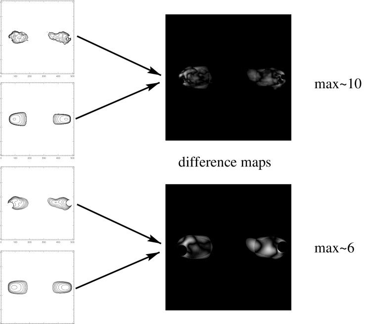
Figure 2: Comparison of the model predictions with the observations of Cygnus A. The contour plots show (from top to bottom) the high resolution map at 1.7 GHz used to compare the model against, the model prediction at high resolution, the convolved map at the same frequency and the corresponding model prediction. The gray scale plots show the difference between model and observations at high (top) and low (bottom) resolution. The ‘max’-values given to the right indicate the maximum deviation of the model in units of the 5$\sigma$ noise level in the observed maps.

Figure 2 also shows the best fitting model maps for both radio lobes and a plot of the differences between model prediction and observation. Note that for convenience both radio lobes are shown in the same plot. However, the model parameters are somewhat different for the two lobes (see Table 1). The differences between the model maps and the observed ones reach 50$\sigma$ in some pixels. These large deviations occur mainly where discrete structure is also seen in the observed maps. This underlines the claim that the model describes the average conditions within the cocoon while it fails in places where there are strong deviations from the mean. It is therefore not surprising that the model fits the lower resolution maps better than the maps with full resolution because the convolution with a larger beam can be viewed to some extent as an averaging process. Figure 2 also shows that the region where flux is measured above the 5$\sigma$ limit in the western lobe extends further along the jet axis then is predicted by the model. At the same time the model prediction is ‘fatter’ than the observed emission. The western radio lobe of Cygnus A gives the impression of being squeezed some way behind the hot spot. It is certainly narrower than its eastern counterpart which is reflected in the model estimates of the geometrical parameters $b_{o}$ and $b_{1}$ (see Table 1). If the lobe is squeezed, this may explain why radio plasma is detected closer to the core. This material has simply a higher backflow velocity than expected from the geometry of the lobe closer to the hot spot. This illustrates that the model has problems in fitting structures deviating from axisymmetry about the jet axis and/or perturbed structures. Note however that the model estimates derived from fitting the surface brightness distribution of the western lobe are close to those obtained from the eastern lobe. The eastern lobe is much more regular in appearance and the irregularities of the western lobe therefore seem to be too weak to significantly alter the model results.

Table 1 shows that there is little difference in the derived model parameters between the high and the low resolution fits. There is still enough information in the variation of the surface brightness in the low resolution maps for the model to produce good results. This is encouraging in the view of the difficulty of obtaining high resolution radio maps of radio sources at high redshift which are probably the most interesting candidates to apply the model to in the future. Because of the large value of $p$, the model is, in the case of Cygnus A, virtually independent of the high energy cut-off of the energy distribution of the relativistic particles. $\gamma_{max}$ is therefore not listed in Table 1.

Most importantly, the best fitting model parameters are close to the ones derived from independent observations. The ‘variations’ of the model parameters given in Table 1 show how much a given parameter can be varied before the $\chi^{2}$-like estimator of the goodness of fit changes by a factor $\sim 2$. The variation of the viewing angle is large because the model only depends on the $\sin$ of this angle and this does not change very much for the large viewing angle of Cygnus A implied by the model. These variations can certainly not be taken as proper error estimates for the predicted model parameters. However, they indicate that the model presented here can be used to produce reasonably firm estimates of the properties of type-II radio sources and their environments.

Table 1: Summary of model results for Cygnus A

		bo	b1	p	$\beta$	$\log(\rho_{o}a_{o}^{\beta})^{\#}$	$\log(Q_{o}^{\ast})$	$\alpha_{V}$
east	low res.	0.24	0.17	2.3	1.42	6.5	39.1	89.8
	high res.	0.27	0.27	2.4	1.41	6.6	39.1	75.5
west	low res.	0.18	0.21	2.4	1.44	7.3	39.1	86.2
	high res.	0.17	0.17	2.4	1.44	7.3	39.1	76.4
‘variation’		0.1	0.05	0.2	0.02	0.3	0.1	20.0
measured					1.45	7.0		75.5

^# $\rho_{o}$ and $a_{o}$ are both measured in SI units.
^∗ in Watts.

References

- [1] \harvarditemBest, Longair & Röttgering1998blr98 Best, P. N., Longair, M. S. and Röttgering, H. J. A. 1998, MNRAS, 295, 549.
- [2] \harvarditemBrunetti et al.1999bcsf99 Brunetti, G., Comastri, A., Setti, G. and Feretti, L. 1999, A&A, 342, 57.
- [3] \harvarditemCarilli, Perley & Harris1994cph94 Carilli, C. L., Perley, R. A. and Harris, D. E. 1994, MNRAS, 270, 173.
- [4] \harvarditemChambers, Miley & van Breugel1990cmb90 Chambers, K. C., Miley, G. K. and van Breugel, W. J. M. 1990, ApJ, 363, 21.
- [5] \harvarditemChyży1997kc97 Chyży, K. T. 1997, MNRAS, 289, 355.
- [6] \harvarditemDunlop & Peacock1990dp90 Dunlop, J. S and Peacock, J. A. 1990, MNRAS, 247, 19.
- [7] \harvarditemHardcastle et al.1998hapr98 Hardcastle, M. J., Alexander, P., Pooley, G. G. and Riley, J. M. 1998, MNRAS, 296, 445.
- [8] \harvarditemHartwick & Schade1990hs90 Hartwick, F. D. A. and Schade, D. 1990, ARA&A, 28, 437.
- [9] \harvarditemKaiser & Alexander1997ka97 Kaiser, C. R. and Alexander, P. 1997, MNRAS, 286, 215.
- [10] \harvarditemKaiser & Alexander1999ka99 Kaiser, C. R. and Alexander, P. 1999, MNRAS, 305, 707.
- [11] \harvarditemKaiser, Dennett-Thorpe & Alexander1997kda97 Kaiser, C. R., Dennett-Thorpe, J. and Alexander, P. 1997, MNRAS, 292, 723.
- [12] \harvarditemKaiser, Schoenmakers & Röttgering1999ksr99 Kaiser, C. R., Schoenmakers, A. P. and Röttgering, H. J. A. 1999, MNRAS, submitted.
- [13] \harvarditemLeahy, Muxlow & Stephens1989lms89 Leahy, J. P., Muxlow, T. W. B. and Stephens, P. W. 1989, MNRAS, 239, 401.
- [14] \harvarditemLeahy & Williams1984lw84 Leahy, J. P. and Williams, A. G. 1984, MNRAS, 210, 929.
- [15] \harvarditemMcCarthy1993pm93 McCarthy, P. J. 1993, ARA&A, 31, 639.
- [16] \harvarditemPress et al.1992ptvf92 Press, W. H., Teukolsky, S.A., Vetterling, W. T. and Flannery, B.P. 1992, Numerical Recipes, Sec. edition, (Cambridge Univ. Press, Cambridge, UK).
- [17] \harvarditemScheuer1974ps74 Scheuer, P. A. G. 1974, MNRAS, 166, 513.
- [18]