Effects of line asymmetries on the determination of solar internal structure

Abstract

Despite the strong evidence that the peaks in the spectrum of solar oscillations are asymmetric, most determinations of mode frequencies have been based on fits of symmetric Lorentzian profiles to the Fourier or power spectra of oscillation time strings. The systematic errors resulting from neglecting the line asymmetry could have serious effects on inversions for the solar internal structure and rotation. Here we analyse artificial data based on simple models of the intrinsic line asymmetry, using GONG mode parameters with asymmetries found by one of us (Rosenthal 1998b ). By fitting Lorentzians to the resulting spectra, we estimate the likely properties of the errors introduced in the frequencies. We discuss whether these frequency shifts have a form similar to the near-surface layers uncertainties and are therefore suppressed in the solar structure inversion. We also estimate directly their contribution, if any, in the solar sound-speed and density determinations using the SOLA technique.

1 Introduction

There is strong evidence that the observed profiles of solar oscillation are asymmetric (e.g. Duvall et al. duvall (1993)). This is thought to be a consequence of the localized nature of the stochastic driving source, possibly combined with a contribution due to noise which is correlated with the driving (e.g. Gabriel gabriel (1994); Abrams & Kumar abrams (1996); Roxburgh & Vorontsov roxburgh (1997); Nigam et al. nigam3 (1998); Rosenthal 1998a b; Nigam & Kosovichev 1998a ). Yet in most analyses of helioseismic data the observed Fourier or power spectra have been fitted with symmetric Lorentzian profiles. This leads to systematic errors in the inferred frequencies, of possibly quite serious effect on the inversion for, e.g., the solar internal structure.

Just how serious will be the effect on the inversion depends on the variation of the frequency shift with mode frequency ($\nu$) and degree ($l$). Our aim then is first to assess how the frequency shift due to fitting asymmetric peaks with Lorentzian profiles varies in the $l-\nu$ plane, and then to consider its effect on structural inversion, specifically a SOLA inversion for sound speed and density. This continues our earlier investigation of this problem (Christensen-Dalsgaard et al. jcd2 (1998), hereafter Paper I).

First we need a model of the line asymmetry. We use the following simple representation of the asymmetric profiles in oscillation power (see also Rosenthal 1998b ):

$$P_{\rm as}(\nu)={\alpha_{1}^{2}\over x^{2}+\alpha_{1}^{2}}\left(1-{2x\over\alpha_{4}}\right)+{\alpha_{1}^{2}\over\alpha_{4}^{2}}+N\;.$$ (1)

Here

$$x={\pi\over\Delta\nu}(\nu-\nu_{0})\;,$$ (2)

where $\Delta\nu$ is the frequency separation between modes of adjacent radial orders. Also, $\nu_{0}$ is the eigenfrequency of the mode, and $\alpha_{4}$ is a measure of the asymmetry. Simple algebra shows that, provided $\alpha_{1}^{2}\ll\alpha_{4}^{2}$, $P_{\rm as}(\nu)$ has a minimum value of $\simeq N$ at $x\simeq\alpha_{4}$. Thus $N$ is a measure of the ratio of noise to signal in the power. In the limit $\alpha_{4}\rightarrow\infty$ we recover a Lorentzian profile with maximum value unity, and with half width at half maximum (measured in terms of $x$) equal to $\alpha_{1}$, sitting on a uniform background of level $N$.

We note that Nigam & Kosovichev (1998a ) presented a formally different, but mathematically essentially equivalent, expression for the asymmetrical line profile. This is characterized by the dimensionless asymmetry parameter $B$ which, in our notation, is given by $B=-\alpha_{1}/\alpha_{4}$.

To estimate the systematic error in the frequency determination we have carried out fits of Lorentzian profiles to timestrings of artificial data, assumed stochastically excited and with a power envelope (see Section 2 for a more precise description) given by Eq. (1). This simulates the analysis of the actual data. The fit results in a determination of the location $x^{\rm(as)}$ of that symmetric Lorentzian which best fits the asymmetric power distribution. From this, the frequency error $\delta^{\rm(as)}\nu$ resulting from the assumption of a Lorentzian profile is obtained as

$$\delta^{\rm(as)}\nu={x^{\rm(as)}\over\pi}\Delta\nu\;.$$ (3)

Of course, $x^{\rm(as)}$ depends on parameters $\alpha_{1}$ (linewidth), $\alpha_{4}$ (asymmetry parameter) and $N$ (background). In order to assess how $\delta^{\rm(as)}\nu$ varies over the $l-\nu$ diagram, we need to know how linewidth, asymmetry parameter and background vary with $l$ and $\nu$. We have used GONG data to estimate the variation of these quantities.

Finally, we have used a SOLA inversion technique to calculate the apparent differences in sound speed and density related to the frequency error $\delta^{\rm(as)}\nu$.

2 Predicted shifts using artificial data

We have considered p-mode power spectra in the vicinity of a single mode. These were constructed, on the assumption of stochastic excitation, as normally distributed Fourier spectra with zero mean and variance given by Eq. (1). To save time and still have good frequency resolution, the simulated data frequency resolution was taken to be $\alpha_{1}$ divided by 5.

Each synthetic power spectrum ($P(\nu_{i})$) was fitted by minimizing the negative of the logarithmic likelihood function ($L$):

$$S({\mathchoice{\mbox{\boldmath$\displaystyle a$}}{\mbox{\boldmath$\textstyle a$}}{\mbox{\boldmath$\scriptstyle a$}}{\mbox{\boldmath$\scriptscriptstyle a$}}})=-\mbox{ln}(L)=\sum_{i}\left\{\log[v({\mathchoice{\mbox{\boldmath$\displaystyle a$}}{\mbox{\boldmath$\textstyle a$}}{\mbox{\boldmath$\scriptstyle a$}}{\mbox{\boldmath$\scriptscriptstyle a$}}},\nu_{i})]+{P(\nu_{i})\over v({\mathchoice{\mbox{\boldmath$\displaystyle a$}}{\mbox{\boldmath$\textstyle a$}}{\mbox{\boldmath$\scriptstyle a$}}{\mbox{\boldmath$\scriptscriptstyle a$}}},\nu_{i})}\right\}\;,$$ (4)

where $v({\mathchoice{\mbox{\boldmath$\displaystyle a$}}{\mbox{\boldmath$\textstyle a$}}{\mbox{\boldmath$\scriptstyle a$}}{\mbox{\boldmath$\scriptscriptstyle a$}}},\nu_{i})$ is the model of the variance of the spectrum, determined by the parameters $\textstyle a$. The model was taken to be a symmetric Lorentzian profile,

$$v({\mathchoice{\mbox{\boldmath$\displaystyle a$}}{\mbox{\boldmath$\textstyle a$}}{\mbox{\boldmath$\scriptstyle a$}}{\mbox{\boldmath$\scriptscriptstyle a$}}},\nu)\ \equiv\ P_{\rm Lor}(\nu)\ =\ A{\gamma^{2}\over(\nu-\nu_{0})^{2}+\gamma^{2}}+B\;,$$ (5)

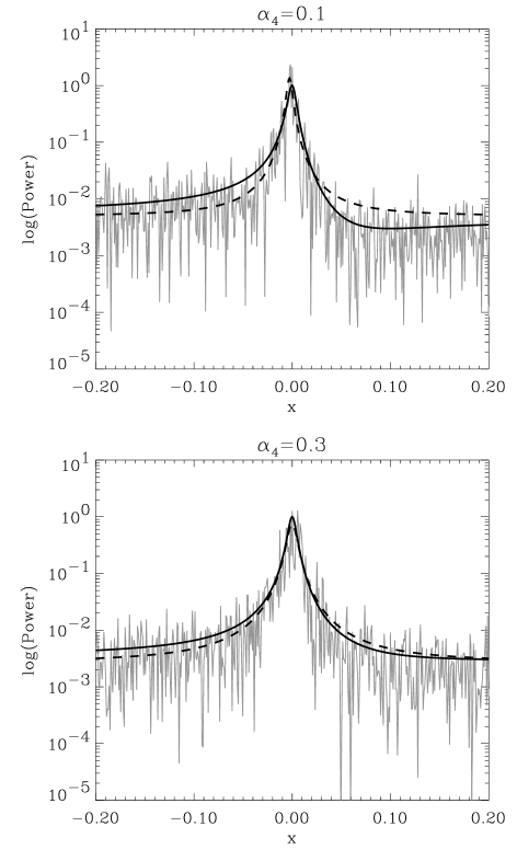
where $A$ is the amplitude, $\nu_{0}$ is the fitted frequency, $\gamma$ is the half width at half maximum and $B$ is the background. As in the fits of real data, the usual parameters were fitted: the central frequency, and the logarithms of the amplitude, linewidth and background noise level. We have fitted over intervals of 100 times $\alpha_{1}$. Fig. 1 shows two examples of ‘peaks’ in such artificial power spectra, and the discrepancy between the true line profile and the fitted Lorentzian.

Figure 1: Synthetic power spectra on a logarithmic scale generated using $\alpha_{1}=0.0045$ and $N=0.003$, as a function of $x$. The two plots are two different realizations using $\alpha_{4}=0.1$ and $0.3$. The heavy continuous lines show the power envelopes $P_{\rm as}$ (cf. Eq. 1) used to generate the spectra, and the dashed lines are the fitted Lorentzian profiles.

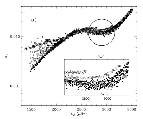
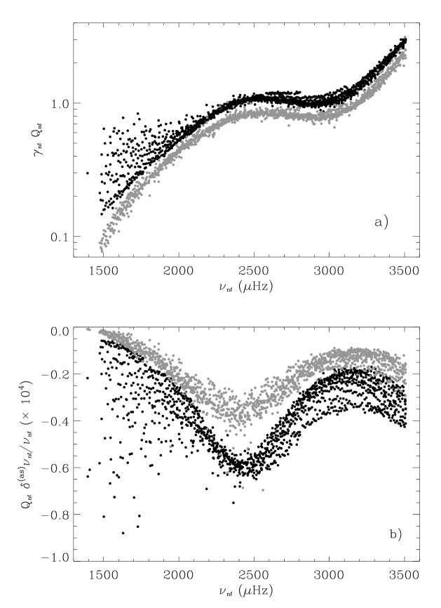
We have used data obtained by the GONG project (e.g. Hill et al. hilletal (1998)) to estimate the parameters of Eq. (1) used to generate the synthetic spectra corresponding to different points in the $l-\nu$ plane. The data were determined in the GONG pipeline by peak-bagging (using Lorentzian profiles) individual modes in the averaged spectra from six 3-month series of observations (GONG months 10-27). For each $(n,l)$ we computed the $m$-averaged frequency, line width (specified in the GONG tables as the FWHM), mode power and background power; based on these averages, we determined the parameters $\alpha_{1}$ and $N$ (assuming the limit $\alpha_{4}\rightarrow\infty$) as well as $\Delta\nu$ in Eqs (1) and (2); the resulting $\alpha_{1}$ and $N$ are illustrated in Fig. 2.

Figure 2: Parameters determining the frequency shifts. Panel a) shows the dimensionless peak width $\alpha_{1}$ (measured in units of the large frequency separation $\Delta\nu$). Panel b) shows the ratio $N$ between the background noise and the peak power. The stars are the extrapolated values for $l\leq 2$. For later reference, modes at low frequency with an $\alpha_{1}$ larger than the general trend are indicated by crosses. The inserts illustrate the dependence of the parameters on mode order $n$, indicated by the symbol types listed in panel b).

Figure 3: Multiplets for which GONG or BiSON (for $l\leq 2$) data have used in this investigation. The crosses correspond to the crosses in Fig. 2.

Unfortunately, the GONG data contain few modes with $l=0$ and none with $l=1$ or 2. To complement our mode set and make a more realistic representation of inversions to infer solar structure, we have extrapolated the parameters $\alpha_{1}$ and $N$ determined through the GONG data for $l<7$ modes to estimate those for $l<3$. The estimation was made for the data set observed by the BiSON group and described by Basu et al. (basu2 (1997)).

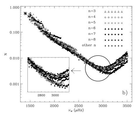
We restrict the analysis to modes with frequency smaller than $3510\,\mu{\rm Hz}$; the mode set contains modes of degree up to 150 (Fig. 3).

The dimensionless asymmetry parameter $\alpha_{4}$ is determined by conditions near the upper turning point of the mode, including the excitation and possibly the effects of correlated noise. Although the details of these processes are as yet poorly understood, it is perhaps not unreasonable to expect that they depend little on degree, at least for the relatively modest degrees considered here; for in this case the horizontal scale of the modes far exceeds the scales of the relevant convective processes. Thus we might expect $\alpha_{4}$ to be a function of frequency alone. We assume that this is precisely the case and estimate $\alpha_{4}$ from the dimensional results for low-degree modes in Fig. 4 of Rosenthal (1998b ), scaling with the value of $\Delta\nu$ for low-degree modes: $\mbox{log}(\alpha_{4})=-2.70+9.52\times 10^{-4}\leavevmode\nobreak\ \nu$, where $\nu$ is given in $\mu$Hz. We note that this $\alpha_{4}$ and our estimate of $\alpha_{1}$ are essentially consistent with the asymmetry parameter $B$ obtained from analysis of MDI (Toutain et al. toutain (1998)) and GOLF (Thiery et al. 1999) data.

We estimate the systematic frequency shifts by fitting symmetric Lorentzians to asymmetric profiles, using the parameter values estimated from the GONG data. For each mode, 1000 simulations were performed; averages of the estimated dimensionless frequency shifts $x^{\rm(as)}/\pi$ are shown in Fig. 4.

Figure 4: Dimensionless frequency shifts $x^{\rm(as)}/\pi$ (i.e., $\delta^{\rm(as)}\nu$, in units of the large frequency separation $\Delta\nu$) obtained by fitting Lorentzians to the asymmetric profile $P_{\rm as}(\nu)$ of Eq. (1), using modal parameters based on GONG data. Each point corresponds to an average of 1000 simulations.

To a considerable extent, $x^{\rm(as)}$ seems to be just a function of frequency. This simple behaviour becomes more understandable if we consider the dependence of the relevant parameters on $l$ and $\nu$. As already stated, it is assumed that the dimensionless asymmetry parameter $\alpha_{4}$ is a function of frequency alone. Fig. 2 shows that the dimensionless line-width $\alpha_{1}$ and the noise-to-signal ratio $N$ for the GONG mode set are predominantly functions of frequency. (That this is so for $\alpha_{1}$ was indeed to be expected, from the physical properties of the damping.) However, they have also some small dependence on order $n$.

The dimensional frequency shifts $\delta^{\rm(as)}\nu$ will have a much stronger $l$-dependence, dominated by the dependence of $\Delta\nu$ on $l$. However, it was shown in Paper I that $\Delta\nu$ is essentially inversely proportional to mode inertia (e.g. Christensen-Dalsgaard & Berthomieu 1991); this, therefore, is also the dominant $l$-dependence of the $\delta^{\rm(as)}\nu$.

Figure 5: Relative frequency error resulting from the assumption of a Lorentzian profile, multiplied by the normalized mode inertia $Q_{nl}$. The continuous curve is a fit to the points of a polynomial of degree 6. The crosses correspond to the crosses in Fig. 2.

3 Effect on Inferred Solar Structure

To test the effect on a solar structure inversion (e.g. for sound speed or density) of the systematic error from fitting asymmetric peaks with Lorentzian profiles, we have run an inversion that assumes the frequency differences between observation and a reference model to arise from differences in internal structure, plus a possible contribution from the surface layers:

$${\delta\nu_{nl}\over\nu_{nl}}=\int K_{c^{2},\rho}^{(nl)}(r){\delta c^{2}\over c^{2}}(r)\ \rm dr +$$

$$\int K_{\rho,c^{2}}^{(nl)}(r){\delta\rho\over\rho}(r)\ \rm dr + \ {{\cal F}_{\rm surf}(\nu_{nl})\over Q_{nl}}\;.$$ (6)

We use a SOLA inversion which seeks to estimate the sound-speed (or density) difference as a function of position within the Sun (see Basu et al. basu1 (1996) for details). Since the whole inversion process is linear, we do not need to create a full set of artificial data: rather, we simply use $\delta^{\rm(as)}\nu_{nl}/\nu_{nl}$ as our data, and this corresponds to the systematic error that would be added to a real inversion of the GONG data due to fitting asymmetric peaks with Lorentzian profiles.

Note that our formulation in Eq. (6) assumes that the difference between the observed and model frequencies in general contains a contribution of the form ${\cal F}_{\rm surf}(\nu_{nl})/Q_{nl}$ where ${\cal F}_{\rm surf}$, which as indicated is a function of frequency alone, is determined by the near-surface errors in the model, and $Q_{nl}$ is the mode inertia normalized by the inertia of a radial mode of the same frequency (e.g. Christensen-Dalsgaard & Berthomieu jcd_berthomieu (1991)). The SOLA inversion allows us to suppress the contribution from the function ${\cal F}_{\rm surf}$ by imposing a constraint that would completely remove such a function if it were a polynomial of degree $\Lambda$ or smaller. Typically we choose $\Lambda=6$: alternatively we can simply choose not to impose this extra constraint at all.

Figure 6: Relative difference in: (a) sound speed and (b) density due to systematic errors in the inferred frequency resulting from the assumption of a Lorentzian profile (Fig. 5). The mode set for the inversions in each panel is the same; the inversions assumed the errors of the observed data in the combined GONG and BiSON data set. The dotted line is for the average over $2l+1$ estimations of $\delta^{\rm(as)}\nu$ (see below), whereas the dashed line used the $\delta^{\rm(as)}\nu$ calculated with MDI linewidths (see below).

Figure 7: Relative difference in: (a) sound speed and (b) density between Sun and the reference model using the observed frequencies calculated by the GONG and BiSON projects (Lorentzian fitting). The dotted line is the solution has been obtained by subtracting the inferred relative differences (circles) in Fig. 6, i.e., it shows the solution ‘corrected’ for the effect of fitting the data with a Lorentzian profile.

If the frequency shifts introduced by mis-fitting the asymmetric peaks were also to be of the form ${\cal F}_{\rm surf}(\nu_{nl})/Q_{nl}$, they too would therefore be suppressed in the inversions. In Fig. 5, we have plotted the relative frequency error resulting from the assumption of a Lorentzian profile, multiplied by the normalized mode inertia $Q_{nl}$. As $Q_{nl}$ is asymptotically related to $\Delta\nu$, Fig. 5 is very similar to Fig. 4. The scattered points at low frequency (crosses) are associated with the scatter in $\alpha_{1}$ (crosses in Fig. 2). The linewidth determination at low frequency is particularly difficult because of its small magnitude. We have looked at other data sets, e.g. MDI data, and this scatter at low frequency is not present, which suggests that it is an artifact of a poor determination (see Fig. 9a, below).

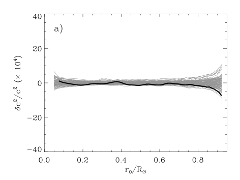
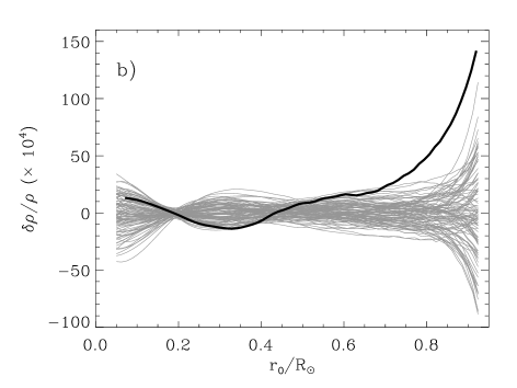
Fig. 5 shows that the relative frequency error due to fitting Lorentzians, when scaled by mode inertia, is in fact largely just a function of frequency; thus one might expect that much of it would be suppressed by the suppression of the surface term in the SOLA inversion. The actual inferred sound-speed and density differences from performing SOLA inversions of $\delta^{\rm(as)}\nu_{nl}$ are illustrated in Fig. 6. For comparison, we show also in Fig. 7 the inferred sound-speed and density differences between the Sun and Model S of Christensen-Dalsgaard et al. (jcd1 (1996)), using the $m$-averaged mode frequencies obtained by the GONG project plus the BiSON mode frequencies for $l<3$ (described in Section 2). For consistency with the results for the solar data, in the inversions we assumed that the errors in the $\delta^{\rm(as)}\nu_{nl}$ were the same as the errors in these observed frequencies. The important conclusion is that the change in the inferred sound speed due to $\delta^{\rm(as)}\nu_{nl}$ is small compared with the total sound-speed difference between the Sun and the model. The same is true of the change in inferred density below the convection zone, for $r<0.7R$. However, it appears that the inference of density in the convection zone is more sensitive to the effects of asymmetry, as described here. The magnitude of the effect can perhaps be better appreciated in Fig. 7. There the dotted lines show the result that would be obtained from inversion of solar frequencies corrected for the effect of asymmetry, i.e., from observed frequencies fitted with an asymmetric profile given by Eq. (1), on the assumption that our representation of asymmetry is correct. The only significant modification from the original solar inference is for $\delta\rho/\rho$ at $r>0.7R$: there we see that the inferred density difference in the convection zone is no longer nearly constant, in contrast with our usual experience with density differences between pairs of solar models (e.g. Christensen-Dalsgaard jcd3 (1996)).

We note that it actually makes rather little difference in this case whether the SOLA inversion explicitly suppresses surface contributions or not: the variation with frequency in Fig. 5 has little effect on the inversion even when the surface constraint is not applied. In fact, even without taking explicitly account of a surface term, the inversion provides some suppression of contributions of this form: this follows from the fact that the near-surface effect of, e.g., $\delta c^{2}/c^{2}$ in Eq. (6) is also of a form similar to the surface term; thus the localization implicit in the inversion leads to a partial elimination of such contributions. (Of course, the surface term in frequency differences between the Sun and adiabatic frequencies of a model is typically more than an order of magnitude larger than the differences in Fig. 5, so it is indeed important to apply a strict surface constraint when inverting real data.)

It follows that the results of the inversions, shown in Fig. 6, are dominated by the scatter of the points in Fig. 5 around the curve fitted as a function of frequency. Much of this scatter could be due to noise in the GONG parameter values. This then affects the inversions in much the same way as random noise in the frequency data. We have carried out inversions of normally distributed random numbers with variances corresponding to the spread in the points in Fig. 5 from the fitted curve (neglecting the low-frequency values shown by crosses), to demonstrate the effect of the scatter on our inversions. The results are shown in Fig. 8, indicating that the sound-speed results are essentially consistent with such a random distribution. In addition, we have verified that the monotonic increase with $r$ in $\delta\rho/\rho$ in the convection zone results from the scattered points at low frequency, shown as crosses in Fig. 5.

Figure 8: Relative difference in: a) sound speed and b) density due to 100 different noise realizations (see text). The thick line is the relative difference due to $\delta^{\rm(as)}\nu$, same as the circles in Fig. 6.

4 Discussion

As described in Section 2, when fitting the observations, the mode parameters were estimated for each ($n,l,m$) and averaged over the $(2l+1)$ different $m$ to give the values for the multiplet ($n,l$). To reproduce the properties of the observations, it would therefore be more realistic to perform $2l+1$ simulations and average the estimated $\delta^{\rm(as)}\nu$, instead of averaging 1000 realizations as considered so far. This will increase the scatter in the frequency shift, especially for low-degree modes. The dotted lines in Fig. 6 show the corresponding sound-speed and density differences. The monotonic decrease in sound-speed and increase in density differences towards the surface are still present, somewhat enhanced for sound speed as a result of the larger scatter in $\delta^{\rm(as)}\nu$. However, the variations are still generally small compared with the total difference between Sun and model (Fig. 7).

The inferred frequency shifts depend rather sensitively on the parameters assumed for the modes, particularly their line widths, and hence the use of parameter values based on just a single data set might be cause for some concern. We have already noted that noise in the GONG parameter determination might have a substantial influence on the inversion results. Another point is that the GONG pipeline may systematically overestimate the linewidths. Evidence for this assertion is shown in Fig. 9a, comparing the GONG linewidths used here with MDI linewidths for a period corresponding to GONG months 29-31 obtained by the MDI Medium $l$ Program (Schou schou (1998)); evidently, the MDI linewidths are systematically smaller than those from GONG. It seems probable that the systematic discrepancy arises from the fact that the MDI parameter determination takes the $m$-leakage into account, whereas the GONG determination did not. (As an aside, we also note that the scatter at low frequency in the GONG data – crosses in Fig. 2a – is not present in the MDI data.)

On the basis of this comparison it would obviously be of interest to repeat our study using parameters obtained from the MDI pipeline. Unfortunately, there is not at the moment a good determination of the background power when using the MDI pipeline (the fit is performed only in a very narrow window around each peak, so that the background far from the peak cannot be determined reliably). However, we have tried using MDI linewidths to estimate $\alpha_{1}$ and GONG data to estimate $N$: the resulting $\delta^{\rm(as)}\nu/\nu$ are shown in Fig. 9b (gray dots) and compared with the results we obtained with GONG linewidths (black dots). As one would expect, the smaller MDI linewidths result in smaller values of $\delta^{\rm(as)}\nu$. Thus, the results in the present study may be pessimistic in the sense that if the GONG linewidths are overestimated, then this will cause us also to overestimate the effects of line asymmetry. Besides, the MDI linewidths do not show a dependence on degree (or order) at given frequency, in contrast to GONG data (cf. Fig. 2a). Thus the dependence of $\delta^{\rm(as)}\nu$ on degree is small; the degree dependence that remains is probably introduced mostly by the $N$ parameter obtained from GONG. The dashed lines in Fig. 6 show the resulting inferred sound-speed and density differences. The monotonic variation towards the surface is substantially smaller than for the full GONG parameters, particularly for density, and has the opposite sign; this confirms our impression that the inferred structural variations in the solar interior (Fig. 6, circles) are probably largely an artifact of the scatter in the GONG parameter determinations, which we have then used in our asymmetry model.

Figure 9: a) Normalized linewidth obtained from GONG (black dots) and from MDI (gray dots) for a period corresponding to GONG months 29-31 by Schou (schou (1998)). b) Relative frequency error resulting from the assumption of a Lorentzian profile multiplied by the normalized mode inertia $Q_{nl}$ using linewidths obtained from: GONG (black dots) and MDI (gray dots).

5 Conclusions

Our principal conclusion is that the frequency shift that arises from erroneously fitting the asymmetric line profiles with symmetric Lorentzians (as is commonly done at present) is rather benign: it is predominantly of the same form as a structural near-surface contribution – viz. of the form ${\cal F}_{\rm surf}(\nu_{nl})/Q_{nl}$, a function of frequency divided by mode inertia, which is largely suppressed in the inversion, and much of the departure from this behaviour is likely to be caused by observational scatter in the GONG mode parameters which form the basis for our study. Thus, although there is some residual error introduced into the sound-speed and density inversions at depth, its magnitude is generally very small. We therefore find no evidence to suggest that ignoring line asymmetry has compromised the helioseismic structural inversions published to date.

One might worry that since the values of $N$ and $\alpha_{1}$ obtained from the GONG tables are themselves the result of a fit of a symmetric Lorentzian profile, they are also subject to systematic error. The symmetric fit picks out the power level far from the peak as being the noise level. This systematically over-estimates the true noise level which is given by the power minimum or trough which lies close to the peak. However, that error depends only on $\alpha_{1}$ and $\alpha_{4}$ and should therefore also be a function only of frequency. On the other hand, the amplitude and line width are only moderately affected by the asymmetry (see Paper I). Hence we do not expect this to affect our conclusions that $x^{\rm(as)}$ is predominantly a function of frequency and that $\delta^{\rm(as)}\nu$ has predominantly the same functional form as a near-surface contribution.

A recently published letter by Toutain et al. (toutain (1998)) purports to show a much more significant effect on the inferred sound speed in the solar core from neglecting line asymmetry when determining mode frequencies. Although we have not considered precisely the same mode set that they did, we view the result of Toutain et al. with some caution. They compared the inversion of mode frequencies obtained by fitting observational data with symmetric Lorentzians with the inversion of mode frequencies in which the low-degree modes only had been fitted with asymmetric profiles. By fitting the low degrees asymmetrically, and the rest symmetrically, it is quite probable that one will artificially introduce an $l$-dependent error that does not scale like inverse mode mass and which will be erroneously interpreted in the inversion as a spatial variation of the structure in the solar core.

We did a similar experiment with our artificial data. In Fig. 10, we compare the inversion of mode frequencies obtained by fitting observational data with symmetric Lorentzians (triangles) with the inversion of mode frequencies which for the low-degree modes ($l\leq 2$) only have been corrected for the effect of asymmetry, by applying our estimates of the frequency shift (circles with error bars). Note that the inversion of the symmetrical fits (triangles) and the inversion of mode frequencies which have all been corrected for the effect of asymmetry (squares) agree quite well in the solar core, as already shown in Fig. 7a. However, using the asymmetrical fits only for $l\leq 2$ modes introduces a change in the solution in the solar core; this confirms our concern that such an inconsistent treatment of asymmetry introduces an artificial $l$-dependence and hence may affect the inversion in the core. We note that the effect obtained here is more modest than that of Toutain et al. (toutain (1998)); the effect we find is quantitatively similar to what has been found by S. Turck-Chièze (private communication). We have been able to make some qualitative comparisons with the asymmetry corrections applied by Toutain et al., thanks to T. Toutain (private communication). It appears that their asymmetry corrections for $l=1$ and $l=2$ are very similar and, encouragingly, these agree with our simulated $\delta^{\rm(as)}\nu$ quite well; but the $l=0$ corrections are rather different. Evidently such an effect would introduce some degree dependence and therefore radial variation into Toutain et al.’s inversion results.

Figure 10: The circles with error bars show the results obtained with asymmetrically fitted low-degree ($l\leq 2$) modes and symmetrically fitted otherwise ($l>2$). The triangles represent the result of the symmetrical (Lorentzian) fits to all modes (same as circles in Fig. 7a) and the squares the asymmetrical fits to all modes (same as dotted line in Fig. 7a). To be compared with Fig. 5 in Toutain et al. (toutain (1998)).

Although we conclude that ignoring line asymmetry has likely not compromised helioseismic structural inversions to date, we should like to emphasize the importance of taking into account the asymmetric profile in the estimation of mode parameters now and in the future. With the SOHO satellite and the GONG network giving us longer time series and with a better signal to noise ratio, the effect of asymmetry on the mode parameter determinations is significant. This is particularly true as we shall be looking for ever more subtle features in the solar interior. Another important reason for fitting an asymmetric profile is the possibility of combining different observables. For example, for solar oscillations observed in Doppler velocity and continuum intensity, the asymmetry in their power spectra has an opposite sign (Nigam & Kosovichev 1998b ) which can lead to different estimates of the mode parameters when fitting a symmetric profile. An inversion of datasets with incompatible frequencies due to different line asymmetries will be seriously compromised, because the combined frequency error will not look like a single near-surface term and will in general be interpreted by the inversion method as a spatial variation inside the Sun. Likewise, it is possible that non-contemporaneous data or data from instruments with different levels of background noise would likewise contain systematic errors with serious consequences for inversions, unless the peakbagging takes line asymmetry into account. We finally note that the determination of the asymmetry, and other parameters of the modes, provides crucial information about the excitation about the solar oscillations (e.g. Rosenthal 1998a; Kumar & Basu 1999; Nigam & Kosovichev 1999).