Critical Comparison of 3-d Imaging Approaches

Abstract

Currently three imaging spectrometer architectures, tunable filter, dispersive, and Fourier transform, are viable for imaging the universe in three dimensions. There are domains of greatest utility for each of these architectures. The optimum choice among the various alternative architectures is dependent on the nature of the desired observations, the maturity of the relevant technology, and the character of the backgrounds. The domain appropriate for each of the alternatives is delineated; both for instruments having ideal performance as well as for instrumentation based on currently available technology. The environment and science objectives for the Next Generation Space Telescope will be used as a specific representative case to provide a basis for comparison of the various alternatives.

L-43, Lawrence Livermore National Laboratory, P.O. Box 808, Livermore, California, 94550

1. Introduction

It is expected that within the year, a decision will be made as to the composition of the suite of science instruments to be deployed on the Next Generation Space Telescope (NGST). It is therefore a particularly good time for a discussion of the relative merits, and appropriate domains of greatest utility for the various 3-d imaging alternatives. There has been, and no doubt will continue to be, a great deal of discussion as to which approach to 3-d imaging is “the best”. There is no single correct answer, of course, since each type of instrument has its own strengths and weaknesses.

It does not seem to be widely known that, in the limiting case of photon statistical noise dominance, the performance of a 3-d imaging spectrometer based on 2-d detector arrays is the same for all architectures (Bennett et al. 1995), whether tunable filter, dispersive, or Fourier transform, provided that the same degrees of freedom are measured. In the following, I will first consider the photon statistics limited case, and show the equivalence between the various architectures. I will then generalize to the performance in the case that detector read noise, dark current, and Zodiacal background are included. I will consider specific parameters that are appropriate for the anticipated NGST environment. Finally, I will offer a suggestion for a hybrid instrument which combines the best features of all of the 3-d architectures, and offers great potential for best meeting the NGST needs.

2. Tunable Filter vs. Dispersive Spectrometer (Ideal Limit)

In comparing between the various options, it is important to assume equivalent detectors. In order to obtain 3-d data using a 2-d detector array, a series of exposures must be made. Consider an $N\times M$ pixel focal plane array, having no “gaps” between the pixel elements. Typical frames for a dispersive imaging spectrometer (DS), and a tunable filter imaging spectrometer (TF) are indicated schematically in Figure 1. In general, it is of course not necessary for the spatial samples observed by the DS to be contiguous, as implied by the arrangement displayed in Figure 1. Nor is it necessary for the spectral samples observed by the TF to be contiguous and non-overlapping, as is also implied by the configuration displayed in Figure 1. Indeed, in some cases, non-contiguous spectral sampling is desirable, and the TF system lends itself much more naturally to this mode of operation. On the other hand, for some questions, the ability to observe non-contiguous spatial samples is very important, and the DS approach, such as with a Multi-Object Spectrometer (MOS), is better suited for such measurements. For the moment, consider the case that the same spatial and spectral samples are covered by both the TF and the DS. Assume that the spectral samples represented by the various pixels along the dispersion direction in the DS correspond exactly both in terms of bandwidth and band center to the series of measurements made by the TF system, and that the spatial samples represented by the various pixels in the TF system similarly correspond exactly to the series of spatial measurements made by the DS system. In this case, if the total observation time is divided equally among the spectral samples for the TF case, and for the spatial samples in the DS case, each cell in the 3-d datacube is observed for the same exposure time, and with the same efficiency. Clearly the signal to noise performance will be the same for both of these configurations.

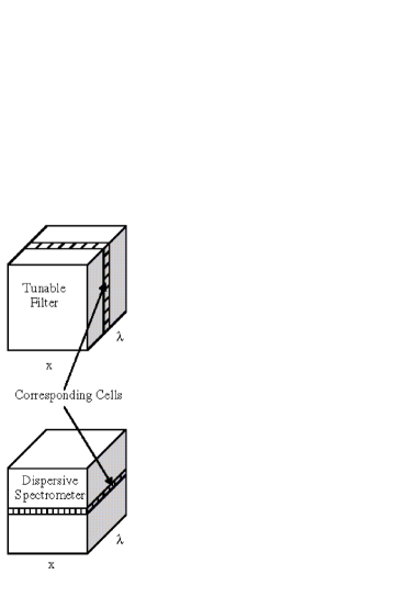
Figure 1.: A schematic comparison between a Tunable Filter Imaging Spectrometer and a Dispersive Imaging Spectrometer.

3. Tunable Filter vs. Fourier Transform Spectrometer (Ideal Limit)

The relation between the performance of an ideal tunable filter spectrometer with an ideal Fourier transform spectrometer is more subtle than that between the tunable filter and the dispersive spectrometer. One simplification, however, is that since the size of the image may be assumed the same for the FT and TF systems, it is only necessary to consider the information content of a single representative detector element obtained via either the TF or the FT system.

It is helpful to consider an analogy with the use of the Modulation Transfer Function (MTF) for the characterization of imaging systems. Consider an “object” spectrum having a sinusoidal intensity variation as a function of frequency. Also assume that this object spectrum is observed with a TF spectrometer having uniformly spaced filter samples, and that all of the filter samples have an equal transmission bandwidth. The “image” spectrum would also have a sinusoidal intensity variation as a function of frequency. In the case that the period of the sinusoidal intensity variation is much smaller than the characteristic width of the TF spectral channels, the “image” spectrum modulations are greatly reduced. Furthermore, if the spacing of the TF spectral samples is not sufficiently dense, the period of the modulations in the “image” spectrum may be altered by “aliasing effects”.

An FT spectrometer, at each of a sequence of retardance settings, directly measures the intensity of a particular sinusoidal intensity variation in the object spectrum. The set of such measurements constitutes an interferogram. In order to compare the information content of TF spectra measured in the frequency domain with FT interferograms measured in the transform domain, it is important to carefully consider the shape of the spectral response of the TF filters, their spacing, and the amount of spectral information content being measured.

In a naive approach to a TF system, it would be assumed that the transmission function for each of the TF filters had a “top hat” shape, i.e. outside the spectral bandpass of a given filter the transmission would be zero, and within a given bandpass the transmission would be unity. Viewed in terms of the response to sinusoidal modulations in the “object” spectrum, such filters have undesirable ramifications, such as contrast reversal for some modulation periods, and aliasing for others. Correspondingly, the most straightforward approach to the acquisition of interferograms by an FT spectrometer, involving equal weighting of each of the retardance measurements, produces effective spectral response functions which have undesirable negative sidelobes. It is important to consider spectral transmission functions which do not have such “sharp corners” as the “top hat” shape for the TF case, and to consider tapered weighting of the interferograms for the FT case.

Consider a sequence of measurements of the intensity of an underlying continuous spectral intensity function $S(\nu)$, dependent on the frequency $\nu$, that is transmitted through a spectral filter $\tau(\nu)$. For a transmission filter centered at $\nu_{0}$, the observed number of photoelectrons would be given by

$$S_{\nu_{0}}=T_{\nu_{0}}\int_{0}^{\infty}S(\nu)\tau(\nu_{0}-\nu)d\nu.$$ (1)

Here the units of spectral radiance $S(\nu)$ are photons Hz^-1 s^-1, the exposure time for the observation is $T_{\nu_{0}}$, in units of s, while the transmission function $\tau(\nu)$ is dimensionless. Also, although the integration limits extend to infinity, this is a purely formal convenience, and in this integral, as in others to follow, the integrand will always be limited to a finite range. The frequency variable, $\nu$, is in units of Hz. (It is sometimes convenient to use the wavenumber equivalent of the frequency, defined by $\nu/c$, and having dimensions of cycles per cm). It is assumed that the quantum efficiency is unity. The peak transmission is assumed to be unity, and the effective width of the transmission filter may be defined by

$$\Delta\nu_{eff}=\int_{0}^{\infty}\tau(\nu)d\nu.$$ (2)

In the case that the spectral radiance function varies slowly over the interval for which $\tau(\nu)$ is significant, the integral in Eq. (1) may be approximated by

$$S_{\nu_{0}}\simeq T_{\nu_{0}}S(\nu_{0})\Delta\nu_{eff}.$$ (3)

The variance in the observed number of photoelectrons, in the statistical noise limit is equal to the total number of photoelectrons detected,

$$var(S_{\nu_{0}})=T_{\nu_{0}}S(\nu_{0})\Delta\nu_{eff}.$$ (4)

Using the relation between the observed counts and the estimate of the underlying spectral radiance function evaluated at $\nu_{0}$ of Eq. (3),

$$var(S(\nu_{0}))={S(\nu_{0})\over T_{\nu_{0}}\Delta\nu_{eff}}.$$ (5)

For comparison with the FT spectrometer case, for which the noise spectrum $var(S(\nu_{0}))$ is independent of $\nu_{0}$, the dwell time $T_{\nu_{0}}$ is taken proportional to $S(\nu_{0})$. (This assumed dwell time variation could of course only be used if the spectrum is known, and would not be applicable to multiple pixels, if they contain different spectra. The impact of varying spectral shape on the comparison between FT and TF spectrometers will be further discussed below.) The constant of proportionality may be determined by requiring that the sum over all $\nu_{0}$ channels yields the total observation time,

$$T_{\nu_{0}}=T_{tot}{S(\nu_{0})\Delta\nu_{0}\over\int_{0}^{\infty}S(\nu)d\nu}.$$ (6)

Here the factor $\Delta\nu_{0}$ is the spacing between the TF spectral samples. For this integration time sequence the spectral variance becomes,

$$var(S(\nu_{0}))={\int_{0}^{\infty}S(\nu)d\nu\over T_{tot}\Delta\nu_{0}\Delta\nu_{eff}}.$$ (7)

With measurements made at the sample spacing $\Delta\nu_{0}=\Delta\nu_{eff}$ this yields

$$var(S(\nu_{0}))={\int_{0}^{\infty}S(\nu)d\nu\over T_{tot}\Delta\nu_{eff}^{2}}.$$ (8)

.

Measurements made at a sample spacing much finer than this produce little additional information about the continuum function $S(\nu)$, since the magnitude of $\Delta\nu_{eff}$ sets a practical limit to the fineness of the resolution recoverable, no matter how fine the sample spacing.

3.1. Derivation of the Basic Fourier Transform Relationships

The intensity of the interference pattern in a dual output port Michelson interferometer, $I(x)$, is a continuous function of the optical path difference $x$, i.e., the retardance, between the two mirrors, related to the continuous spectral intensity detected, $S(\nu)$, by the integral,

$$I_{\pm}(x)={1\over 2}\int_{0}^{\infty}S(\nu)(1\pm cos(2\pi\nu x/c))dx.$$ (9)

The two output ports correspond to the two sign values, with the “+” sign corresponding to the output port for which the two interfering beams are in phase at zero optical path difference (ZPD), and the “-” sign corresponding to the output port with out of phase beams at ZPD. As before, the product $S(\nu)d\nu$ has units of counts per second. Eq. (9) is valid for a perfectly compensated, perfectly efficient beam splitter. Real beam splitters have dispersion and are not perfectly efficient, but these complications are easily dealt with in practice. It is convenient to form the sum and difference of the signals from the two output ports of the interferometer. These two quantities are given by the integrals,

$$I_{\Sigma}(x)=\int_{0}^{\infty}S(\nu)d\nu,$$ (10)

and

$$I_{\Delta}(x)=\int_{0}^{\infty}S(\nu)cos(2\pi\nu x/c))dx.$$ (11)

Note that the summed signal is independent of the optical path difference $x$, and is simply given by the integrated spectral intensity. Thus at each retardance setting of the interferometer the full broad band image is measured. This is because, in the absence of absorption losses, every photon entering the interferometer goes to one or the other of the exit ports. The difference signal, at the zero retardance position also becomes equal to the same full band intensity integral.

This feature of the summed signal from an FT system suggests that a desirable hybrid of FT and TF may be obtained by simply having a tunable filter placed in the optical train of an imaging FT spectrometer. In this case, the sum of the two output ports of the FT spectrometer provides the unmodulated full intensity of the light that has passed through the tunable filter. In addition, higher resolution spectral imaging may be obtained at the same time. In this hybrid approach, the summed output will be called the “panchromatic” output of the FT, while the transform of the difference output will be called the “spectral” output of the FT instrument.

In general, it is advantageous to have the dwell time depend on retardance in order to tailor the effective spectral line shape and maximize data collection efficiency. This is typically done for radio astronomy, but is not typically done for laboratory FTIR spectroscopy. A typical interferogram would consist of a set of $N$ discrete samples of the continuous function $I(x)$, symmetric about the point $x=0$, each observed with dwell time $T_{n}$.

$$I_{n}=T_{n}I_{\Delta}(x_{n}),{\rm\ with\ }x_{n}=n\delta x,\ n\ {\rm in\ the\ range\ }[-N/2+1,N/2].$$ (12)

Discrete Fourier transformation results in periodogram estimates, $S_{k}$, at integer multiples $k$ of a fixed frequency spacing $\delta\nu$, approximately related to the continuous function $S(\nu)$ by

$$S_{k}\simeq T_{0}S(\nu_{k})\delta\nu{\rm\ with\ }\nu_{k}=k\delta\nu,\ k\ {\rm in\ the\ range\ }[-N/2+1,N/2].$$ (13)

The approximate relation between the discrete spectral estimate and the continuous spectral function is accurate to the extent that the continuous spectral function varies sufficiently slowly in the neighborhood of the discrete sample point at $\nu=\nu_{k}$. This condition is similar to that used in writing expression (3) for the TF case. The spectral sample spacing $\delta\nu$ and the interferogram sample spacing $\delta x$ are related by $\delta\nu=c/(N\delta x)$. The $S_{k}$ values are given by the discrete Fourier transform,

$$S_{k}={2\over N}\sum_{n=-N/2+1}^{N/2}I_{n}exp(-i2\pi kn/N).$$ (14)

The inverse discrete Fourier transform is

$$I_{n}={1\over 2}\sum_{k=-N/2+1}^{N/2}S_{k}exp(i2\pi kn/N).$$ (15)

The normalization used for the Fourier transform pair displayed in expression (14) and (15) has been chosen to most directly reflect the continuum relation of expression (11).

It follows from the convolution theorem that the spectral line shape, $S^{res}$, for a particular set of dwell times $T_{n}$ is proportional to a Fourier transform,

$$S_{k}^{res}={1\over T_{tot}}\sum_{n=-N/2+1}^{N/2}T_{n}exp(-i2\pi kn/N).$$ (16)

With this normalization, the peak of the resolution function at $k=0$ is equal to unity. This resolution function plays the same role as the transmission function $\tau(\nu)$ for the TF case. Just as for the TF case, an effective width for the resolution function may be defined by summing over all $k$ values,

$$\Delta\nu_{eff}=\delta\nu\sum_{k=-N/2+1}^{N/2}S_{k}^{res}={T_{0}\over T_{tot}}N\delta\nu.$$ (17)

Although the case of uniform integration times is simplest for the FT spectrometer, and indeed is the most common mode of operation of laboratory FTIR instruments, it is not the most efficient. Furthermore, for purposes of comparison with a TF spectrometer, the resolution function (a sinc function) has negative sidelobes, which cannot be realized by a physical transmission filter function $\tau(\nu)$. There are many choices for the dwell time series which produce non-negative spectral line shape functions which can be physically realized as transmission filter profiles. One of the simplest is the triangular apodization series, defined by

$$T_{n}=T_{0}\left(1-{2|n|\over N}\right),\ n=-N/2+1,...,0,...N/2.$$ (18)

The spectral line shape that results from this weighting is a sinc-squared function.

3.2. Fourier Transform Spectrometer Noise

For a real interferogram, the discrete spectrum is hermitian, i.e., $Re(S_{k})=Re(S_{-k})$. While $Im(S_{k})=-Im(S_{-k})$. The point $k=N/2$ corresponds to the Nyquist frequency. For a perfectly compensated beam splitter, with 100% modulation efficiency and no noise, the interferogram will also be symmetric. A real, symmetric interferogram produces a real, symmetric spectrum. Noise in the interferogram is real, and produces a hermitian contribution to the calculated spectrum. Noise in the interferogram is not necessarily symmetric, however, and thus contributes to both the real and the imaginary parts of the calculated spectrum. By virtue of the linear relation between interferogram and spectrum, and with the notation that primed quantities represent noise contributions, the spectral noise is simply the Fourier transform of the interferogram noise.

$$S^{\prime}_{k}={2\over N}\sum_{n=-N/2+1}^{N/2}I^{\prime}_{n}exp(-i2\pi kn/N).$$ (19)

For a dual ported interferometer, with focal plane detectors having equivalent noise performance characteristics, specifically having a noise variance given by the sum of a read noise term, $n_{r}^{2}$, plus a statistical noise term, the difference interferogram measurements have the noise characteristics:

$$<I^{\prime}_{n}>=0.<I^{\prime}_{n}I^{\prime}_{m}>=\delta_{n,m}\left(2n_{r}^{2}+{T_{n}\over T_{0}}I_{0}\right).$$ (20)

In the above expressions, the angle brackets represent an ensemble average. It is assumed that the noise is uncorrelated for different samples of the interferogram. The statistical properties of the spectral noise that follow from (19) and (20) are

$$<S^{\prime}_{k}>=0,<Re(S^{\prime}_{k})^{2}>=\left({2\over N}\right)^{2}\sum_{n=-N/2+1}^{N/2}\left(2n_{r}^{2}+{T_{n}\over T_{0}}I_{0}\right)cos^{2}(2\pi kn/N).$$ (21)

Since for finite $k$ values, the $cos^{2}$ factor in expression (21) oscillates much more rapidly as a function of $n$ than the factor $T_{n}$, it may be well approximated by 1/2. With this approximation, the spectral noise becomes independent of $k$, i.e., it is “white”. The variance of the measured continuum spectrum thus is given by

$$var(S(\nu_{k}))={<Re(S^{\prime}_{k})^{2}>\over(T_{0}\delta\nu)^{2}}={2\over(\Delta\nu_{eff}T_{tot})^{2}}\left(2Nn_{r}^{2}+T_{tot}\int_{0}^{\infty}S(\nu)d\nu\right).$$ (22)

In the case that of a 1-sided interferogram, with samples

$$I_{n}=T_{n}I_{\Delta}(x_{n}),\ {\rm with\ }x_{n}=n\delta x,\ n\ {\rm in\ the\ range\ }[0,N_{1}-1].$$ (23)

The variance of the measured continuum spectrum is given by

$$var(S(\nu_{k}))={1\over(\Delta\nu_{eff}T_{tot})^{2}}\left(2N_{1}n_{r}^{2}+T_{tot}\int_{0}^{\infty}S(\nu)d\nu\right).$$ (24)

Although it may appear that the decrease in the variance has come “for free”, there is really no greater information content, since the density of independent spectral samples is only half as great in the spectrum derived from the 1-sided interferogram. The difference in the variance between 1-sided and 2-sided interferograms can be most easily derived (for perfectly symmetrical interferograms) by averaging each -n interferogram sample with the +n sample, and computing the Fourier transform of the resulting 1-sided interferogram. The statistical noise would be reduced by a factor of $1/\sqrt{2}$ for each interferogram sample, and since only half as many readouts would be required, the readout noise would be reduced a factor of two.

Expression (24), in the absence of read noise, matches expression (8) obtained for the TF case. Expression (22), similarly matches expression (7) for the TF case with a sampling interval $\Delta\nu_{0}={1\over 2}\Delta\nu_{eff}$, as is appropriate for the more dense sampling in frequency space. The interesting fact that the only spectral line shape parameter that enters into the spectral noise for a Fourier transform spectrometer is the effective width, $\Delta\nu_{eff}$ , is novel, to this author’s knowledge (e.g., Griffiths & de Haseth, 1986). The remarkable equivalence of the noise performance over all of the various types of ideal imaging spectrometers may perhaps be interpreted in terms of an “information theory” argument.

4. Zodiacal Background and Detector Noise Terms

The Zodiacal light produces a substantial limiting background flux for NGST. For a 1 AU orbit, thermal emission from dust dominates at wavelengths longer than about 3.5 $\mu$m, while for wavelengths shorter than this, scattered sunlight produces the dominant background. An estimate of this background spectrum is displayed in Figure 2. The zodiacal background flux is constant, to good approximation, over the range of frequencies from 3,000 to 10,000 cycles/cm, at a level of approximately $3x10^{-4}$ photon cm s^-1. Detector noise performance levels anticipated for deployment on NGST are displayed in the table below. The impact on the performance of the various 3-d imaging systems generated by these background sources are displayed in the next section.

Table 1.: NGST Detector Performance Expectations

Case	Single Frame Read	Dark Current
	Noise, $n_{1}$ ($e^{-}$)	$I_{d}$ ($e^{-}$ s-1)
Current	15	0.1
Goal	3	0.02

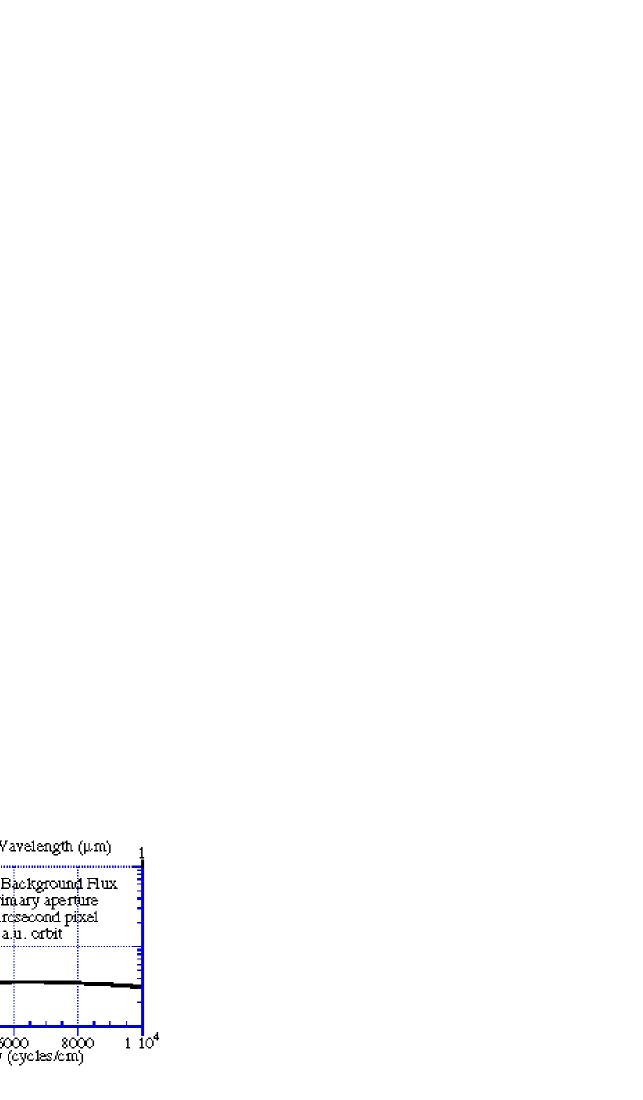
Figure 2.: The magnitude of the Zodiacal light background expected for NGST in a 1AU orbit.

5. The Impact of Backgrounds on 3-d Spectrometers

The signal to noise ratio, SNR, in the presence of backgrounds, (including detector dark current, $I_{d}$, read noise, $n_{r}$, and zodiacal background, $Z(\nu)$), for the TF and the DS case, is given by

$$SNR={\eta\;QE(\nu)\;S(\nu)\Delta\nu_{eff}T_{\nu}\over\sqrt{((QE(\nu)(S(\nu)+Z(\nu))\Delta\nu_{eff})+I_{d})T_{\nu}+n_{r}^{2}}}.$$ (25)

In this expression, the $QE(\nu)$ factor represents not only the quantum efficiency of the detector elements themselves, but also includes all other system transmission losses, such as non-unity reflectance for reflecting surfaces, and non-zero absorption losses in any transmitting elements. In general this factor may vary spectrally, and in a fairly complex manner. Dispersive gratings, for example, will have reflective losses for off-blaze angles of reflection. Tunable filters have absorptive losses which tend to be greater for high resolution broadly tunable filters. The efficiency factor $\eta$ in expression (25) encapsulates all effects which lower the signal level without concomitantly lowering the background level, such as surface scattering losses, for example.

The signal to noise ratio in the presence of backgrounds for the FT case is obtained from expression (24) by including the modulation efficiency factor and QE effects, adding both the zodiacal background and the detector dark current contributions to the total number of photoelectrons observed, and including readout noise,

$$SNR={\eta\;QE(\nu)\;S(\nu)\Delta\nu_{eff}T_{tot}\over\sqrt{(\int QE(\nu)(S(\nu)+Z(\nu))\delta\nu+2I_{d})T_{tot}+2Nn_{r}^{2}}}.$$ (26)

This expression reduces to the expression for the spectral SNR of Graham, et al. (1998), under the simplifying assumptions made in that article. Fourier transform spectrometers have a modulation efficiency factor which enters into the $\eta$ efficiency factor for the spectrally resolved $SNR$, but not into the pan-chromatic $SNR$. The magnitude of the read noise term which appears in expressions (25) and (26) depends on the number of non-destructive readouts of the detector array that are averaged to determine the estimated photo-current $I$ for a particular spectrometer setting. This number is a compromise between integrating the photo-current for a longer time, which lowers the variance, and averaging more readouts, which decreases the amount of time available for integration. To good approximation, the optimum number of readouts is determined by $I$, the single frame read noise, $n_{1}$ and the time it takes to read out the array, $\Delta_{t}$, via

$${\rm Optimal\ Number\ of\ Reads}={n_{1}\over\sqrt{I\Delta t}}$$ (27)

Therefore, $n_{r}^{2}=n_{1}\sqrt{I\Delta t}$.

Estimates of plausible realistic values for the system $QE$ and $\eta$ values are listed in Table 2 for operation in the $K$ band. The NGST main telescope transmission was calculated assuming that all of the mirrors are gold coated. The dispersive spectrometer values are taken from curves computed by Satyapal (1999), for the $K$ band at either $R$=1000 or $R$=10,000, although they are somewhat optimistic compared to the values routinely obtained at large ground based telescopes. The tunable filter efficiencies are estimated on the basis of Northrop Grumman tunable Fabry-Perot performance values (Madonna & Ryan). The somewhat surprisingly low QE for the tunable filter may be attributed to the fact that the effective number of surfaces seen by the transmitted light is approximately equal to the finesse, and thus extremely high quality surfaces are necessary to produce low losses at high finesse. The FT modulation efficiency corresponds to that of a 30^∘ incident angle NIR-MidIR CsI Bomem beamsplitter (Villemaire 1999).

Table 2.: Spectrometer Efficiency Assumptions ($K$ band)

Case	QE	$\eta$
	detector+optics
TF	0.35	1
DS	0.6	0.7
FT	0.7	0.95

The Noise Equivalent Flux Density, $NEFD$, at a particular significance level is derived from the $SNR$ equations by solving for the flux $S$ which produces the given significance level. The NEFD for observations in the K band at 2.2 $\mu$m, (as one example) at the 10 $\sigma$ level, for a variety of imaging spectrometer options are displayed in Figure 3 as a function of spectral resolution. From these curves, for a particular problem of interest, it is easy to select the optimum instrumental configuration.

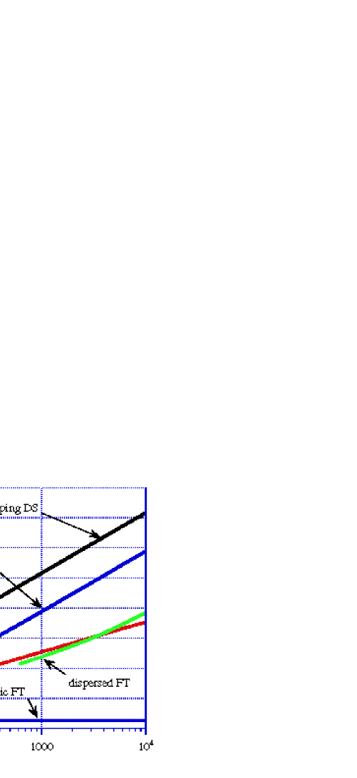
Figure 3.: The Noise Equivalent Flux Density for a variety of 3d imaging approaches are displayed. The detector performance parameters are: 15 e^- read noise per readout, 0.1 e^- s^-1 dark current. All observations extend over the $K$ band, centered at 2.2 $\mu$m, and assume a total observation time of $10^{5}$ s. The time per readout is assumed to be 1 s. The QE and efficiency, $\eta$, values are those of Table 2 for each of the systems. TF = tunable filter, DS=dispersive spectrometer, FT=Fourier transform spectrometer. The “mapping DS” corresponds to scanning over a number of field of view settings equal to the number of spectral channels for the TF at each resolution, and thus has an NEFD equal to that of the TF spectrometer. It is only through this factor that the array size enters, as was shown in figure 1. The single setting TF corresponds to the observation of a full field of view, but through only a single filter. The panchromatic FT line indicates the NEFD sensitivity for the full K band imaging that is obtained as a function of the resolution of the imaging FT system. This sensitivity is almost independent of the resolution, since the loss of exposure time involved in the multiple readouts for the spectroscopy is a small fraction of the total observation time. The dispersed FT curve corresponds to the addition of an $R$ = 630 prism in the collimated space of the imaging FT optical train, and the addition of a slit at an image plane. The dispersed FT case with slit, would not produce the panchromatic FT full field imaging. A dispersed FT operated ala a slit-less objective prism would produce the panchromatic FT full field imaging.

At the lowest spectral resolution At the lowest spectral resolution, all of the 3-d instruments converge to the performance of an $R$=5, $K$ band camera. At the highest spectral resolution, the DS has the best performance for spectroscopy, although only for the small number of objects that may be contained “within the slit”. This fact is the basis for the current pre-eminence of Multi-Object Spectrometers and Integral Field Units in high resolution astronomical spectroscopy. For the purpose of imaging in a very narrow, single emission line band, the TF provides an $NEFD$ performance equivalent to that of the DS, but for every pixel in the field of view. For the purpose of obtaining complete spectra for every pixel in the field of view, the FT instrument substantially outperforms the TF or the “mapping DS”, (whose performance becomes essentially equivalent to the TF). The point of equivalence between the imaging FT and the DS comes at the point for which the number of settings of the DS is equal to the square of the ratio in performance between the single setting DS and the imaging FT.

For any resolution, the imaging FT instrument has the advantage that not only are spectra obtained for every pixel in the field of view, but that very deep K-band imaging (in this example, but it could be $J$, $H$, $L$, etc. or the entire 0.6-5.5 $\mu$m range) is simultaneously acquired. In many of the design reference missions for NGST, the data for both deep imaging and spectroscopy may be acquired simultaneously. The fact that such imaging is produced for every resolution setting of the FT instrument is indicated in Figure 3 by the lowest $NEFD$ curve labeled “panchromatic FT”.

At the highest spectral resolution, the relatively strong signals required imply that for many fields of interest to NGST, the angular density of observable objects will be small enough that at most one object is expected per field of view. In this situation, it is not helpful to obtain spectra for every pixel in the field of view, and the spatial multiplexing of the imaging FT is not useful.

A very interesting hybrid approach (e.g., Beer 1992) is possible, however, which takes advantage of the best features of all of the 3-d imaging approaches. This is the combination of an objective prism with an imaging FT spectrometer. A relatively modest dispersion across one dimension of the image plane serves to reduce the spectral bandpass acceptance that is involved in the noise term for the FT spectrometer. With a slit at an image plane, the “panchromatic” output of the FT spectrometer would yield the same results as an ordinary prism spectrometer, while the Fourier transformed interferograms would enable much higher spectral resolution at much reduced NEFD. The curve labeled “dispersed FT” in Figure 3 corresponds to the assumption that a prism of dispersion equal to that of CaF₂ is placed in the collimated space of an imaging FT, and that the slit width is equal to one pixel. For objects which have much higher intensity than their surroundings, slit-less objective prism style measurements are also possible.

There are slight displacements of the curves for the various spectrometer, and imaging spectrometer configurations, depending on the choices for the detector performance parameters, and system efficiency values. Using the NGST “goal” detector performance parameters instead of the “current” performance values slightly improves the sensitivity of the TF, the DS, and the dispersed FT, but produce very little change in the imaging FT case. On the other hand, using grating efficiencies closer to those typical of ground based telescopes, lowers the DS curve, but not the TF, the imaging FT, or the dispersed FT curves. The mapping DS curve does not take into account any in-efficiencies with the precision re-pointing between observations.

In conclusion, the ability of a single instrument concept, composed of a filter wheel, programmable slit, dispersive prism, and Michelson interferometer, to deliver the performance of a wide field camera, the performance of a moderate resolution, full field imaging spectrometer, and the performance of a high resolution, limited field spectrometer seems to make this choice nearly obligatory for NGST.

This work was performed under the auspices of the U.S. Department of Energy under Contract No W-7405-Eng-48. I thank my IFIRS colleagues for many stimulating discussions and astronomical tutoring: J. R. Graham, M. Abrams, J. Carr, K. Cook, A. Dey, R. Hertel, N. Macoy, S. Morris, J. Najita, A. Villemaire, E. Wishnow, and R.Wurtz. I also thank J. Mather for the provocative suggestion to consider the dispersed FT option.

References

C. L. Bennett, M. R. Carter and D. J. Fields, “Hyperspectral Imaging in the Infrared Using LIFTIRS”, Proc. SPIE, 2252, 274 (1995)

R. Beer, “Remote Sensing by Fourier Transform Spectrometry”, J. Wiley & Sons, N.Y., (1992), p.67.

J.R. Graham, M. Abrams, C.L. Bennett, J. Carr, K. Cook, A. Dey, J. Najita and E. Wishnow, “The Performance and Scientific Rationale for an Infrared Imaging Fourier Transform Spectrograph on a Large Space Telescope”, PASP, 110, 1205, (1998).

P. R. Griffiths and J. A. de Haseth, “Fourier Transform Infrared Spectroscopy”, J. Wiley & Sons, N.Y., (1986), and many other references, do treat the SNR performance of Fourier transform spectrometers, but only in terms of a relatively poorly defined resolution parameter.

R. Madonna and R. Ryan, 1999, private communication.

S. Satyapal, from anonymous ftp site:grisly.gsfc.nasa.gov, in directory:
out.going/shobita/spectrometer_trade

A. Villemaire, 1999, private communication.