Anisotropic inverse Compton scattering from the trans–relativistic to the ultra–relativistic regime and application to the radio galaxies.

Abstract

The problem of the anisotropic Inverse Compton scattering between a monochromatic photon beam and relativistic electrons is revisited and formally solved without approximations. Solutions are given for the single scattering with an electron beam and with a population of electrons isotropically distributed, under the assumption that the energy distribution of the relativistic particles follows a simple power law as it is the case in many astrophysical applications. Both the Thomson approximation and the Klein-Nishina regime are considered for the scattering of an unpolarized photon beam. The equations are obtained without the ultra–relativistic approximation and are compared with the ultra–relativistic solutions given in the literature. The main characteristics of the power distribution and spectra of the scattered radiation are discussed for relevant examples. In the Thomson case for an isotropic electron population a simple formula holding down to the mildly–relativistic energies is given.

As an application the formulae of the anisotropic inverse Compton scattering are used to predict the properties of the X and $\gamma$–ray spectra from the radio lobes of strong FR II radio galaxies due to the interaction of the relativistic electrons with the incoming photons from the nucleus. The dependence of the emitted power on the relativistic electron energy distribution and on its evolution with time is discussed.

PACS: 95.30.Cq; 95.30.Gv; 98.38.Am; 98.54.Gr; 98.70.Qy

1 Introduction

Inverse Compton (IC) scattering is one of the most common radiative processes in astrophysics. The papers of Jones (1968) and Blumenthal & Gould (1970) provide the basic theory, while both exact expressions and useful approximations for interaction rates, mean scattered energies, and dispersion about the mean energies are given by Coppi & Blandford (1990). The computations reported in these papers have been performed by supposing an isotropic distribution of the incident photon momenta. However, there are astrophysical situations in which the photon momenta are anisotropically distributed so that the standard equations are not sufficient.

From a theoretical standpoint, Baylis et al.(1967) showed that the Compton spectrum (emitted over the total solid angle) from a beam of ultra–relativistic electron population ($N_{e}(\gamma)\propto\gamma^{-\delta}$) in the Thomson approximation is independent on the incoming photon distribution being for all considered cases $\propto\epsilon^{-(\delta-1)/2}$. The anisotropic inverse Compton (AIC) equations describing the scattering between a photon beam and isotropic relativistic electrons in the Thomson approximation were obtained by Bonometto et al.(1970) for a power law energy distribution of ultra–relativistic electrons. Aharonian & Atoyan (1981) obtained the general redistribution function describing the scattering probability into a given direction of a monochromatic incoming photon beam scattered by isotropic monochromatic relativistic electrons. Furthermore, by integrating the redistribution function over a population of ultra–relativistic electrons with a power law energy distribution ($N_{e}(\gamma)\propto\gamma^{-\delta}$) they obtained the analytical expression of the spectrum (in terms of hypergeometric series) and showed that it presents the same shape of that derived from an isotropic illumination (i.e. $\propto\epsilon^{-(\delta-1)/2}$ in the Thomson approximation and $\propto\epsilon^{-\delta}ln(\epsilon\epsilon_{0})$ in the Klein–Nishina regime; $\epsilon_{0}$ being the energy of the seed photons). More recently, Nagirner & Poutanen (1993) have obtained the redistribution matrix for Compton scattering of polarized incoming photon beams and, by integrating the redistribution function over a power law energy spectrum of ultra–relativistic electrons in the Thomson approximation, they showed the equivalence between their results and those of Bonometto et al.(1970).

All the formulae of astrophysical interest reported in these papers are obtained by making use of the ultra–relativistic limit. As a consequence, they are not useful to the detailed study of astrophysical situations in which also trans–relativistic and mildly–relativistic electrons are involved.

More recently Brunetti et al.(1997) have treated the AIC Thomson scattering of a photon beam by an isotropic electron distribution not restricted to the ultra–relativistic limit.

The AIC has been considered in several specific astrophysical situations. The Compton losses suffered by electrons moving in a bath of anisotropic seed photons was studied both in the Thomson approximation and in the Klein–Nishina case and was used to produce optical and gamma–ray emission from the pulsars (see Morini 1981, 83 and reference therein). With reference to the hard X–ray properties of compact sources (AGNs and galactic black hole candidates), Ghisellini et al. (1991) have derived (Thomson approximation) the angular distribution of the power and the spectrum of the hard IC radiation emitted by a relativistic electron located at the center of an hemispherical bowl, or cap, uniformly radiating soft X–rays (the emission region was assumed to be optically thin and the AIC scattering is taken to be isotropic in the electron rest frame). Dermer & Schlickeiser (1993) and Böttcher et al. (1997) have derived approximate solutions describing the AIC scattering of incoming photons from an accretion disc with the ultra–relativistic electrons in the relativistic jets of AGNs.

Recently, Moskalenko & Strong (1999) have discussed the effect due to the anisotropic distribution of the incoming photons on the gamma–ray emission from interstellar photons IC scattered by cosmic–ray electrons in the Galaxy. This has been achieved by numerically integrating a redistribution function, in the Klein–Nishina regime, that was obtained by considering the scattered photons as unidirectionally emitted in the direction of the electrons. However, this approximation is strictly valid only in the ultra–relativistic case, which is the one of interest in the mentioned paper.

The inverse Compton scattering of collimated streaming particles with a surrounding bath of soft photons emitted by the disc–torus would produce high energy photons in AGNs and/or galactic X–ray binaries (Bednarek & Kirk 1995, Protheroe et al. 1992). Furthermore the same mechanism has been used to model the gamma ray emission in the MeV blazar objects (Bednarek 1998). In order to better describe the emission pattern of all these astrophysical situations general exact analytical expressions would be useful.

The aim of the present paper is to investigate the AIC single scattering in the general case: from the trans–relativistic to the ultra–relativistic limit, both in the Klein–Nishina case and in the Thomson approximation. General formulae of astrophysical interest are derived. Specifically, we will consider the scattering of a photon beam with an electron beam (Sect.3) and with an isotropic distribution of electron momenta (Sect.4). In Sect.2 we define the basic geometry of the scattering and obtain general relationships from the scattering between a monochromatic photon beam and an electron. In Sect.4 we also compare our results with those of Bonometto et al.(1970) and Aharonian & Atonyan (1981) for the ultra–relativistic AIC and with the isotropic ultra–relativistic inverse Compton case (Blumenthal & Gould 1970).

As an application, in Sect.5 we use our general AIC equations of Sect.4 to study the X–to–gamma ray spectrum of the powerful radio galaxies deriving from the AIC scattering of the nuclear IR–to–UV photons from a hidden quasar by the relativistic electrons in the radio lobes. In particular we argue that the detection of such emission with the new generation X–ray telescopes (Chandra, XMM) can provide important information about the magnetic field strength, the energy density, distribution and aging of the relativistic particles in the radio galaxies.

2 IC scattering between a photon beam and a single electron

We assume a scattering geometry such that the momenta of the incoming and scattered photon and of the electron are described by the four-vectors (Fig.1):

$$P={{\epsilon}\over c}(1,0,0,1)$$ (1)

$$P_{1}={{\epsilon_{1}}\over c}(1,k_{j})$$ (2)

$$P_{e}=mc\gamma(1,\beta e_{j})$$ (3)

Figure 1: The geometry of the scattering: the incoming monochromatic (energy $\epsilon$) photon beam propagates along the Z–axis and the photons are scattered to an energy $\epsilon_{1}$ in the direction ($\theta_{SC},\phi_{SC}$) by electrons with momenta in the ($\theta,\phi$) direction.

$\epsilon$ and $\epsilon_{1}$ being the incoming and scattered photon energies, $k_{j},\,e_{j}$ ($j=1,2,3$) the unit vector components in spherical coordinates, $m$ the electron mass and $\beta=v/c$ the electron velocity.

With these assumptions the incoming photon density is given by:

$$n(\epsilon,\Omega_{ph})d\epsilon d^{2}\Omega_{ph}={n\over{2\pi}}\delta(\epsilon-\epsilon_{0})\delta(cos\theta_{ph}-1)d\epsilon d^{2}\Omega_{ph}$$ (4)

$\epsilon_{0}$ being the assumed incoming photon energy, $\delta$ the Dirac–function.

It is well known that in the Compton scattering the tetra–vector components of the incident and scattered photons in the lab frame and in the electron frame (primed) are related by (Rybicki & Lightman 1979, Pozdnyakov et al. 1983):

$$\epsilon_{1}=\gamma(1+\beta e_{j}^{\prime}k_{j}^{\prime})\epsilon_{1}^{\prime}$$ (5)

$$\epsilon^{\prime}=\gamma(1-\beta e_{3})\epsilon$$ (6)

$$\epsilon_{1}^{\prime}=\epsilon^{\prime}(1+\epsilon^{\prime}(1-cos\theta^{\prime}_{SC})/mc^{2})^{-1}$$ (7)

where $\gamma$ is the Lorentz factor of the electron.

In general the inverse Compton emissivity in the lab frame may be obtained by the manifold integral (Blumenthal & Gould 1970):

$$j(\Omega_{SC},\epsilon_{1})=\int d\epsilon^{\prime}d^{2}\Omega^{\prime}_{ph}d^{2}\Omega_{e}d\gamma{{d^{3}n^{\prime}(\epsilon^{\prime},\Omega^{\prime}_{ph};\epsilon,\Omega_{ph})}\over{d\epsilon^{\prime}d^{2}\Omega^{\prime}_{ph}}}{{d^{2}\Omega^{\prime}_{SC}d\epsilon^{\prime}_{1}dt^{\prime}}\over{d^{2}\Omega_{SC}d\epsilon_{1}dt}}$$

$$\cdot{{d^{3}\sigma}\over{d^{2}\Omega^{\prime}_{SC}d\epsilon^{\prime}_{1}}}\epsilon_{1}c\,N_{e}(\gamma,\Omega_{e})$$ (8)

where $d^{3}n^{\prime}$, the photon number density in the electron frame, can be easily derived from the relativistic invariant $dn/\epsilon$ (Blumenthal & Gould 1970). For a monochromatic ($\epsilon_{0}$) photon beam moving along the Z–axis (Eq.4) it is:

$${{d^{3}n^{\prime}(\epsilon^{\prime},\Omega^{\prime}_{ph};\epsilon,\Omega_{ph})}\over{d\epsilon^{\prime}d^{2}\Omega^{\prime}_{ph}}}={{n}\over{2\pi}}{{\epsilon^{\prime}}\over{\epsilon}}{{d^{2}\Omega_{ph}d\epsilon}\over{d^{2}\Omega^{\prime}_{ph}d\epsilon^{\prime}}}\delta(cos\theta_{ph}-1)\delta(\epsilon-\epsilon_{0})$$ (9)

$d\sigma$ is the differential Compton cross section, in our case the unpolarized Klein–Nishina cross section (Berestetskii et al. 1982):

$${{d^{3}\sigma}\over{d^{2}\Omega^{\prime}_{SC}d\epsilon^{\prime}_{1}}}={{r_{0}^{2}}\over 2}({{\epsilon^{\prime}_{1}}\over{\epsilon^{\prime}}})^{2}({{\epsilon^{\prime}_{1}}\over{\epsilon^{\prime}}}+{{\epsilon^{\prime}}\over{\epsilon^{\prime}_{1}}}-1+cos^{2}\theta^{\prime}_{SC})\cdot$$

$$\delta\left(\epsilon^{\prime}_{1}-{{\epsilon^{\prime}}\over{1+\epsilon^{\prime}(1-cos\theta^{\prime}_{SC})/mc^{2}}}\right)$$ (10)

$N_{e}(\gamma,\Omega_{e})$ is the electron number per energy and solid angle. In this case it is formally written as:

$$N_{e}(\gamma,\Omega_{e})d\gamma d^{2}\Omega_{e}=\delta^{2}(\Omega_{e}-\Omega^{0}_{e})\delta(\gamma-\gamma_{0})d\gamma d^{2}\Omega_{e}$$ (11)

and $cos\theta^{\prime}_{SC}$, the scattering angle in the electron frame, is derived by a Lorentz transformation of Eqs.(1–2) along the electron direction :

$$cos\theta^{\prime}_{SC}=1+{{k_{3}-1}\over{\gamma^{2}(1-\beta e_{3})(1-\beta e_{j}k_{j})}}$$ (12)

The velocity of the electron that scatters a photon from energy $\epsilon$ to $\epsilon_{1}$ is derived by combining Eqs.(5–7) and making use of the relativistic transformation of the angles ($\beta e_{j}k_{j}\neq 1$):

$$\beta=\{(e_{j}k_{j}-\epsilon e_{3}/\epsilon_{1})^{2}+({{1-k_{3}}\over{mc^{2}}}\epsilon)^{2}\}^{-1}\{(1-{{\epsilon}\over{\epsilon_{1}}})(e_{j}k_{j}-{{\epsilon e_{3}}\over{\epsilon_{1}}})+$$

$${{1-k_{3}}\over{mc^{2}}}\epsilon\{(e_{j}k_{j}-{{\epsilon e_{3}}\over{\epsilon_{1}}})^{2}+({{1-k_{3}}\over{mc^{2}}}\epsilon)^{2}-(1-{{\epsilon}\over{\epsilon_{1}}})^{2}\}^{1\over 2}\}$$ (13)

that in the Thomson approximation (i.e. $\gamma\epsilon(1-k_{3})<<mc^{2}$) becomes

$$\beta\simeq{{\epsilon_{1}-\epsilon}\over{\epsilon_{1}e_{j}k_{j}-\epsilon e_{3}}}$$ (14)

The Compton emissivity is readily obtained by Eqs.(8–12) and (5–7) and well known relativistic transformations:

$$j(\Omega_{SC},\epsilon_{1})={{r_{0}^{2}cn}\over{2\gamma_{0}^{2}}}{{\epsilon_{1}}\over{L_{1}}}\delta(\epsilon-\epsilon_{0})\{(1+{{\epsilon_{1}}\over{mc^{2}}}{{k_{3}-1}\over{\gamma_{0}L}})^{-1}+[1+{{k_{3}-1}\over{\gamma_{0}^{2}LL_{1}}}]^{2}$$

$$+{{\epsilon_{1}}\over{mc^{2}}}{{k_{3}-1}\over{\gamma_{0}L}}\}$$ (15)

where $L=1-\beta_{0}e_{3}^{0}$, $L_{1}=1-\beta_{0}e_{j}^{0}k_{j}$, $\beta_{0}$ is given by Eq.(13) with $e_{j}$ and $e_{3}$ replaced with the assumed electron coordinates ($e^{0}_{j}$ and $e_{3}^{0}$ respectively) and

$$e_{j}^{0}k_{j}={1\over{\beta_{0}}}\{1-{{\epsilon}\over{\gamma_{0}mc^{2}}}(k_{3}-1)-{{\epsilon}\over{\epsilon_{1}}}L\}$$ (16)

In the Thomson approximation Eq.(15) becomes the much more simple:

$$j(\Omega_{SC},\epsilon_{1})\simeq{{r_{0}^{2}cn}\over{2\gamma_{0}^{2}}}{{\epsilon_{1}}\over{L_{1}}}\delta(\epsilon-\epsilon_{0})\{2+2{{k_{3}-1}\over{\gamma_{0}^{2}LL_{1}}}+({{k_{3}-1}\over{\gamma_{0}^{2}LL_{1}}})^{2}\}$$ (17)

with $\beta_{0}$ given by Eq.(14) and

$$e_{j}^{0}k_{j}\simeq{1\over{\beta_{0}}}\{1-{{\epsilon}\over{\epsilon_{1}}}L\}$$ (18)

3 IC scattering between photon and electron beams

As previously assumed the photons propagate along the Z–axis. In this Section the direction of the electron beam is defined by the coordinates $e_{3}\equiv e_{3}^{0}\equiv cos\,\theta_{e}^{0}$ and $\phi\equiv\phi_{e}^{0}$.

The electron number density is formally given by:

$$N_{e}(\gamma,\Omega_{e})d\gamma d^{2}\Omega_{e}=K_{e}f(\gamma)\delta^{2}(\Omega_{e}-\Omega_{e}^{0})d\gamma d^{2}\Omega_{e}$$ (19)

where $K_{e}$ and $f(\gamma)$ are the number density and energy distribution of the electrons.

In this case given $\epsilon_{0},\,\epsilon_{1}$, the electron direction $e_{j}$ and the scattered photon direction $k_{j}$, only one electron energy ($\,\tilde{\gamma}\,$) satisfies the conservation laws. As a consequence the $\delta$–function appearing in Eq.(15) can be written as:

$$\delta(\epsilon-\epsilon_{0})=\delta(\gamma-\tilde{\gamma})\beta\gamma^{3}J$$ (20)

where $\tilde{\gamma}=(1-\tilde{\beta}^{2})^{-1/2}$ is given by Eq.(13) with $\epsilon_{0}$ instead of $\epsilon$, while the Jacobian of $\beta$ with respect to $\epsilon$ is:

$$J=\{(e_{j}k_{j}-\epsilon e_{3}/\epsilon_{1})^{2}+((1-k_{3})\epsilon/mc^{2})^{2}\}^{-1}\{2\beta[{{e_{3}}\over{\epsilon_{1}}}(e_{j}k_{j}-{{\epsilon e_{3}}\over{\epsilon_{1}}})$$

$$-({{1-k_{3}}\over{mc^{2}}})^{2}\epsilon]+{{1-k_{3}}\over{2mc^{2}}}({{\epsilon d\Phi/d\epsilon}\over{\Phi^{1\over 2}}}+2\Phi^{1\over 2})-{{e_{j}k_{j}+e_{3}-2{{\epsilon e_{3}}\over{\epsilon_{1}}}}\over{\epsilon_{1}}}\}$$ (21)

with $\Phi=((1-k_{3})\epsilon/mc^{2})^{2}+(e_{j}k_{j}-\epsilon e_{3}/\epsilon_{1})^{2}-(1-\epsilon/\epsilon_{1})^{2}$.

The Compton emissivity is obtained by integrating Eq.(15) over the electron distribution (Eq.19). By making use of Eqs.(20–21) and well known relativistic transformations, the integration yields:

$$j(\Omega_{SC},\epsilon_{1})={{cr_{0}^{2}}\over{2}}nK_{e}\epsilon_{1}\tilde{\beta}_{0}\tilde{\gamma}_{0}f(\gamma=\tilde{\gamma}_{0})\tilde{F}_{0}\tilde{J}^{0}(1-\tilde{\beta}_{0}e_{j}^{0}k_{j})^{-1}$$ (22)

Figure 2: The geometry of the scattering as seen along the X–axis. The incoming photon beam and the scattering electron beam are shown together with the emission cones for $e_{3}^{0}<e_{3}^{\ast}$ and $e_{3}^{0}>e_{3}^{\ast}$.

where $\tilde{\beta}_{0}$ is given by Eq.(13) with the assumed electron coordinates $e_{j}^{0}$ and the incoming photon energy $\epsilon_{0}$ replacing the general $e_{j}$ and $\epsilon$ respectively. $\tilde{J}^{0}$ is given by Eq.(21) with $e_{j}^{0}k_{j}$, $e_{3}^{0}$, and $\tilde{\beta}_{0}$ replacing $e_{j}k_{j}$, $e_{3}$ and $\beta$, respectively, and where

$$\tilde{F}_{0}=\{1+{{k_{3}-1}\over{{\tilde{\gamma_{0}}^{2}}(1-\tilde{\beta}_{0}e_{3}^{0})(1-\tilde{\beta}_{0}e_{j}^{0}k_{j})}}\}^{2}+{{\epsilon_{1}}\over{mc^{2}}}{{k_{3}-1}\over{\tilde{\gamma}_{0}(1-\tilde{\beta}_{0}e_{3}^{0})}}$$

$$+\{1+{{\epsilon_{1}}\over{mc^{2}}}{{k_{3}-1}\over{\tilde{\gamma}_{0}(1-\tilde{\beta}_{0}e_{3}^{0})}}\}^{-1}$$ (23)

Eq.(22) can be used to calculate the emission due to AIC scattering between a streaming population of relativistic electrons and seed photons emitted by a small region (e.g., a star close to the jet or a hot spot in the accretion disk) in AGNs or galactic X–ray binaries. To describe with high accuracy much more common astrophysical situations the solution can also be easily obtained by numerically integrating over the distributions of the photon and electron momenta.

In order to describe the AIC emitted power and spectrum and the changes introduced by the non ultra–relativistic scattering kinematics, we have to assume an energy distribution of the electron population. Let us assume a simple power law energy distribution, $f(\gamma)=\gamma^{-\delta}$, so that the results of this section can be compared with those in which the electron momenta are isotropically distributed (next section). It should be born in mind, however, that there are no known simple mechanisms providing a power law energy distribution in accelerated electron beams (Fermi mechanisms in general work with isotropic electrons momenta).

The AIC emissivity is simply obtained by replacing $f(\gamma=\tilde{\gamma}_{0})$ with ${\tilde{\gamma}_{0}}^{-\delta}$ in Eq.(22).

It can be noticed that the emitted power vanishes when $\tilde{\gamma_{0}}$ goes to infinity ($\delta>1$). Electrons of increasing energy are required to scatter the photons to a given energy $\epsilon_{1}$ at larger angles from the electron beam, up to a maximum angular distance for which $\beta=1$. Therefore photons of energy $\epsilon_{1}$ are scattered in the line of sight only if the angular distance of the electron beam is sufficiently small. Since the scattering problem is symmetric with respect to the Z–axis, it is simpler to study the spatial distribution of the scattered radiation by assuming that the electron beam lies on the (Y–Z) plane. From Eq.(13), with $sin\,\phi_{SC}=sin\,\phi_{e}^{0}=1$, and $\epsilon=\epsilon_{0}$, one finds that the limiting condition $\tilde{\beta}_{0}=1$ is obtained at two extremes in $k_{3}$ (Fig.2):

$$k_{3}(\pm)=e_{3}^{0}[(1-\epsilon_{0}(1-e_{3}^{0})/\epsilon_{1}]\pm\{(1-(e_{3}^{0})^{2})$$

$$\cdot(1-(1-{{\epsilon_{0}}\over{\epsilon_{1}}}(1-e_{3}^{0}))^{2})\}^{1/2}$$ (24)

Figure 3: The emitted power as a function of the scattering angle for the IC scattering between a photon and an electron beam in the Thomson approximation (solid lines) and with the Klein–Nishina equations (dotted lines). The curves are normalized to the maximum in the Thomson approximation. The electron beam is positioned at $\theta_{e}$(rad)=2.10 and $\phi_{e}=\pi/2$. The upper and lower (solid and dotted) curves correspond respectively to $\delta$= 2.5 and 5.0, while the assumed initial and scattered photon energies are $\epsilon_{0}=10^{3}$eV and $\epsilon_{1}=10$MeV.

Similarly, by releasing the condition $\sin\phi_{SC}=1$, one obtains the extremes in $\phi_{SC}$ by imposing the condition $k_{3}(+)=k_{3}(-)$. If $\theta_{e}^{0}$ is large enough, the emission cone may comprise the Z–axis. The angle of the electron velocity at which this happens is derived from Eq.(24) by setting $k_{3}(-)=-1$:

$$e^{*}_{3}={{-1+\epsilon_{0}/\epsilon_{1}}\over{1+\epsilon_{0}/\epsilon_{1}}}$$ (25)

For $e_{3}^{0}\geq e_{3}^{*}$ the scattered directions on the (Y–Z) plane are comprised in the interval $k_{3}(+)<k_{3}<k_{3}(-)$ and $\phi_{SC}=\pi/2$, while for $e_{3}^{0}<e_{3}^{*}$ the scattered directions are bounded by $-1<k_{3}<k_{3}(+)$ and $\phi_{SC}=\pi/2$ and $-1<k_{3}<k_{3}(-)$ and $\phi_{SC}=3\pi/2$ (Fig.2).

Figure 4: The calculated spectrum from IC scattering between a photon and an electron beam is shown in arbitrary units for different scattering angles both in the Thomson approximation (solid line) and in the Klein–Nishina scattering (dotted line). We have assumed $\delta$=2.5 and an incoming photon energy $\epsilon_{0}=10^{3}$ eV. The assumed scattering angles from the bottom to the top of the diagram are: $\theta_{SC}$ (rad)= 2.20, 2.15, 2.13, 2.11 with the electron beam positioned at $\theta_{e}^{0}$(rad)=2.10 and $\phi_{e}^{0}=\pi/2$.

In the Thomson limit Eq.(22) becomes:

$$j(\Omega_{SC},\epsilon_{1})\simeq{{cr_{0}^{2}}\over{2}}nK_{e}{{\epsilon_{1}^{2}(k_{3}-1)^{2}}\over{\epsilon_{0}\,(\epsilon_{1}-\epsilon_{0})}}(1-{1\over{\tilde{\gamma_{0}}^{2}}})\tilde{\gamma_{0}}^{-\delta+1}\{{1\over{(k_{3}-1)^{2}}}+$$

$$({1\over{k_{3}-1}}+{{(\epsilon_{1}-\epsilon_{0})^{2}}\over{\epsilon_{0}\epsilon_{1}(e^{0}_{j}k_{j}-e^{0}_{3})^{2}}}{1\over{\tilde{\gamma_{0}}^{2}}})^{2}\}$$ (26)

where $\tilde{\gamma_{0}}$ and $\tilde{\beta_{0}}$ are given by Eq.(14) with $e_{j}$ replaced by the assumed electron beam coordinates $e^{0}_{j}$ and with $\epsilon$ replaced by $\epsilon_{0}$. Furthermore it can be readily shown that in the Thomson approximation the emitted pattern has the same boundaries of the Klein–Nishina case.

An example of the emitted power as a function of the scattering angle, both in the Thomson approximation and in the Klein–Nishina case, is represented in Fig.3 for two different values of the electron spectral index. Relatively more power is channeled at larger scattering angles with decreasing $\delta$. The broadening in the emitted power distribution in the case of low values of $\delta$ is due to the contribution of the high energy electrons that emit along relatively large values of $\theta^{\prime}_{SC}$.

Due to the Compton recoil the energies of the electrons that are required to scatter incoming photons ($\epsilon_{0}$) up to an energy $\epsilon_{1}$ in the Klein–Nishina regime are larger than those in the Thomson approximation. As a consequence the emitted power in the Klein–Nishina regime is more depressed in the case of a steeper energy distribution of the electrons (as it is $\delta=5$ in Fig.3).

The emitted power per unit frequency and solid angle as a function of the emitted energy is represented in Fig.4 for different scattering angles both in the Thomson approximation and in the Klein–Nishina case. The very sharp cut-off in the emitted spectrum is simply due to the kinematics of the scattering and only weakly depends on the electron differential spectrum. Such feature represents the portion of the emitted spectrum contributed by the electrons with $\beta$ approaching to unity and with the emitted photons moving along the boundaries of the scattered cones.

In Fig.4 it is seen that the difference between the Thomson approximation and the Klein–Nishina scattering becomes larger at small scattering angles (with respect to the direction of the electron beam) and increases with the energy of the scattered photons. Actually, for each scattering configuration this difference follows a quite complicated trend being smaller both at low and at high emitted energies and larger at intermediate energies. The trend is due to the difference between the Thomson and the KN cross sections but, because of the Compton recoil, it is also sensitive to the electron energy distribution (see Brunetti 1998 for further details).

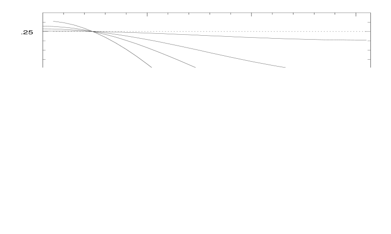
Figure 5: The calculated spectral index ($j\propto\nu^{-\alpha}$) of the spectrum from a scattering between a monochromatic photon beam and an electron beam with a power law energy distribution ($\delta=2.5$). In the scattering the photons are emitted in the direction of the electron beam. From the bottom of the diagram we have reported the spectral index by assuming respectively $\epsilon_{1}/\epsilon_{0}$=50, 100, 200, 1000. The dotted line is the spectral index in the ultra–relativistic case (Eq.28).

A relevant example is the Thomson spectrum in the direction of the electron beam ($e_{j}^{0}k_{j}=1$ and $k_{3}=e_{3}^{0}$). In this case from Eq.(26) the Compton emissivity is:

$$j(e_{3}^{0},\epsilon_{1})\simeq{{cr_{0}^{2}}\over{2}}nK_{e}{{\epsilon_{1}^{2}(\epsilon_{1}-\epsilon_{0})}\over{\epsilon_{0}(\epsilon_{1}-e_{3}^{0}\epsilon_{0})^{\delta+1}}}(1-e_{3}^{0})^{{\delta-1}\over 2}\{1+(1-$$

$$({{\epsilon_{1}-\epsilon_{0}}\over{\epsilon_{1}-e_{3}^{0}\epsilon_{0}}})^{2}{{2\epsilon_{1}\epsilon_{0}-(1+e_{3}^{0})\epsilon_{0}^{2}}\over{\epsilon_{1}\epsilon_{0}}})^{2}\}$$

$$\cdot\{2\epsilon_{1}\epsilon_{0}-(1+e_{3}^{0})\epsilon_{0}^{2}\}^{{\delta-1}\over 2}$$ (27)

Figure 6: The calculated spectral index of the spectrum integrated over $4\pi$ from a scattering between a monochromatic photon beam and an electron beam with a power law energy distribution ($\delta=2.5$) is shown as a function of the ratio $\epsilon_{1}/\epsilon_{0}$. From the top to the bottom of the diagram the electron beam direction is $\theta_{e}$= 0.5, 1.5, 2.0, 2.5, 3.0 (rad), while is taken $\phi_{e}=\pi/2$. The spectral index is computed with 5 eV step ($\epsilon_{0}$=1 eV); in the ultra–relativistic limit it should be $\alpha=0.75$.

In the ultra–relativistic limit Eq.(27) can be expanded in series for $\epsilon_{1}>>\epsilon_{0}$ to get the much more simple:

$$j(e_{3}^{0},\epsilon_{1})\rightarrow cr_{0}^{2}nK_{e}2^{{\delta-1}\over 2}(1-e_{3}^{0})^{{\delta-1}\over 2}({{\epsilon_{1}}\over{\epsilon_{0}}})^{-{{\delta-3}\over 2}}$$ (28)

Now, as one can notice from Eqs.(5–7) if $\theta_{SC}<<1$ then $\tilde{\gamma_{0}}>>1$, however, the ultra–relativistic condition $\epsilon_{1}>>\epsilon_{0}$ is not satisfied. As a consequence although in the case $e_{3}^{0}\simeq 1$ is $\tilde{\gamma_{0}}\rightarrow 1$, the spectrum differs from the so–called ultra–relativistic case as it can be noticed from Eqs.(27–28).

The spectrum per unit solid angle in the mildly–relativistic case (Eq.27) is rather complicated. In Fig.5 its slope is shown as a function of the electron beam direction and of $\epsilon_{1}/\epsilon_{0}$; it is also compared with the ultra–relativistic value (Eq.28).

The power emitted by the electron beam over $4\pi$ can be compared with the formulae giving the emitted power in the case of isotropic inverse Compton scattering given in the literature (Jones 1968, Blumenthal & Gould 1970, Rybicki & Lightman 1979). In the ultra–relativistic case the integration of Eq.(26) over $\Omega_{SC}$ yields:

$$j(\epsilon_{1})\rightarrow\pi cr_{0}^{2}nK_{e}({{\epsilon_{1}}\over{\epsilon_{0}}})^{-{{\delta-1}\over 2}}2^{{{\delta+3}\over 2}}(1-e_{3}^{0})^{{{\delta+1}\over 2}}{{\delta^{2}+4\delta+11}\over{(\delta+1)(\delta+3)(\delta+5)}}$$ (29)

the spectrum is a power law as in Baylis et al.(1967). In the mildly–relativistic case the spectrum is harder for large angles between the incoming photon and the electron beam, while it is softer at small angles (Fig.6).

4 IC scattering between a photon beam and an isotropic electron distribution

In the case of isotropic distribution the electron number density per energy and solid angle is:

$$N_{e}(\gamma,\Omega_{e})d\gamma d^{2}\Omega_{e}=(4\pi)^{-1}K_{e}f(\gamma)d\gamma d^{2}\Omega_{e}$$ (30)

The emissivity is given by integrating Eq.(15) over the angular and energy distribution of the scattering electrons. The integral over $\Omega_{e}$ can be performed by following the method given in Aharonian & Atoyan (1981); one finds:

$$j(k_{3},\epsilon_{1})={{K_{e}r_{0}^{2}\epsilon_{1}^{2}c}\over{4\epsilon_{0}^{2}}}\int{{f(\gamma)}\over{\beta\gamma^{2}}}\{{{2\epsilon_{0}}\over{(\epsilon_{0}^{2}+\epsilon_{1}^{2}-2\epsilon_{0}\epsilon_{1}k_{3})^{1/2}}}+$$

$$({{\epsilon_{0}(1-k_{3})}\over{mc^{2}}}-2{{mc^{2}}\over{\epsilon_{1}}}-2{{(mc^{2})^{3}}\over{\epsilon_{0}\epsilon_{1}^{2}(1-k_{3})}}){\cal R}(\epsilon_{0},\epsilon_{1},\gamma,k_{3})$$

$$+({{(\gamma-\epsilon_{1}/mc^{2})\epsilon_{1}/mc^{2}+\gamma\epsilon_{0}/mc^{2}+\epsilon_{1}\epsilon_{0}k_{3}/(mc^{2})^{2}}\over{[(\gamma-\epsilon_{1}/mc^{2})^{2}(1-k_{3})^{2}+1-k_{3}^{2}]^{3/2}}}$$

$$+{{(\gamma+\epsilon_{0}/mc^{2})\epsilon_{0}/mc^{2}+\gamma\epsilon_{1}/mc^{2}-\epsilon_{1}\epsilon_{0}k_{3}/(mc^{2})^{2}}\over{[(\gamma+\epsilon_{0}/mc^{2})^{2}(1-k_{3})^{2}+1-k_{3}^{2}]^{3/2}}})$$

$$\cdot{{1-k_{3}}\over{\epsilon_{0}\epsilon_{1}^{2}}}(mc^{2})^{3}\}nd\gamma$$ (31)

where the function

$${\cal R}(\epsilon_{0},\epsilon_{1},\gamma,k_{3})=[(\gamma-\epsilon_{1}/mc^{2})^{2}(1-k_{3})^{2}+1-k_{3}^{2}]^{-{{1}\over 2}}$$

$$-[(\gamma+\epsilon_{0}/mc^{2})^{2}(1-k_{3})^{2}+1-k_{3}^{2}]^{-{{1}\over 2}}$$ (32)

The lower limit of the integral Eq.(31) is given by the minimum energy of the electrons that can scatter an incident photon ($\epsilon_{0}$) to an energy $\epsilon_{1}$ in the direction $\Omega_{SC}$.

The minimum velocity of the electrons is obtained by minimizing Eq.(13) with respect to the electron directions ($e_{j}$, i.e. $\theta_{e},\phi_{e}$). Given that the distribution of the scattering electrons is isotropic, it is equivalent to describe the emitted spectrum with reference to any plane containing the incoming photon momenta (the Z–axis). For simplicity of notation we study the scattering properties on the (Y–Z) plane, so that $k_{1}=0$, $k_{2}=(1-k_{3}^{2})^{1/2}$, and the electrons having the lowest energy to make the scattering are those moving on the (Y–Z) plane i.e. with $\phi_{e}=\pi/2$ (i.e. $e_{1}=0$).

We find that Eq.(13) is minimized by electrons having directions :

$$e_{3}(\pm)=\pm\{1+{{k_{2}^{2}}\over{(k_{3}-\epsilon_{0}/\epsilon_{1})^{2}}}\}^{-1/2}$$ (33)

with $e_{3}(+)$ for $k_{3}\geq\epsilon_{0}/\epsilon_{1}$ and $e_{3}(-)$ for $k_{3}<\epsilon_{0}/\epsilon_{1}$. By combining Eqs.(13) and (33) one finds $\beta_{min}$ and $\gamma_{min}=\{1-\beta_{min}^{2}\}^{-1/2}$. It should be noticed that Eq.(33) holds whatever the electron and the photon energy may be, i.e. both in the Thomson approximation and in the Klein–Nishina case, from the ultra–relativistic limit down to the trans–relativistic case.

In the Thomson approximation, from Eqs.(14) and (33), we find:

$$\gamma_{min}\simeq\{1+{{(\epsilon_{1}-\epsilon_{0})^{2}}\over{2\epsilon_{0}\epsilon_{1}(1-k_{3})}}\}^{1/2}$$ (34)

that becomes the simplest $\gamma_{min}\rightarrow(\epsilon_{1}/2\epsilon_{0}(1-k_{3}))^{1/2}$ in the ultra–relativistic case (Bonometto et al. 1970), and the well known $\gamma_{min}=1/2\sqrt{\epsilon_{1}/\epsilon_{0}}$ in the ultra–relativistic isotropic Thomson scattering (taking $k_{3}=-1$).

4.1 The Thomson approximation

In the literature it is usually assumed a momentum–power law energy distribution of the relativistic electrons $f(\gamma)=\beta^{-1}(\beta\gamma)^{-\delta}$ since it is that expected from Fermi acceleration mechanisms. It deviates from a simple energy–power law in the non ultra–relativistic case.

In this section our aim is to derive AIC equations from the trans–relativistic to the ultra–relativistic regime and to compare our findings with the ultra–relativistic equations in the literature. As a consequence, in order to evidence the changes in the AIC emitted spectrum and pattern introduced only by the non ultra–relativistic scattering kinematics, in this section, we adopt a simple energy–power law distribution $f(\gamma)=\gamma^{-\delta}$ down to trans–relativistic energies. The case of a general $f(\gamma)$ is discussed in Appendix A where a simple semi–analytical solution is given. The case of the distribution $f(\gamma)=\beta^{-1}(\beta\gamma)^{-\delta}$ is discussed in Appendix B and is compared with the results of this section.

From Eq.(31) the integration in the Thomson case yields:

$$j(k_{3},\epsilon_{1})\simeq{{K_{e}r_{0}^{2}c}\over{4}}({{\epsilon_{1}}\over{\epsilon_{0}}})^{2}n\{{{2{\cal I}_{0}}\over{(({{\epsilon_{1}}\over{\epsilon_{0}}})^{2}-2k_{3}{{\epsilon_{1}}\over{\epsilon_{0}}}+1)^{1\over 2}}}-$$

$$2(1-k_{3})^{-1}(1+{{\epsilon_{0}}\over{\epsilon_{1}}}){\cal I}_{3/2}+$$

$$(1-k_{3})^{-2}[(1+{{\epsilon_{0}}\over{\epsilon_{1}}})(3k_{3}-{3\over 2})-{3\over 2}({{\epsilon_{1}}\over{\epsilon_{0}}}+({{\epsilon_{0}}\over{\epsilon_{1}}})^{2})]{\cal I}_{5/2}$$

$$+{5\over 2}(1-k_{3})^{-2}[3(1+{{\epsilon_{0}}\over{\epsilon_{1}}})+({{\epsilon_{1}}\over{\epsilon_{0}}}+({{\epsilon_{0}}\over{\epsilon_{1}}})^{2})]{\cal I}_{7/2}\}$$ (35)

where

$${\cal I}_{0}={1\over{\sqrt{\pi}}}\sum_{i=0}^{\infty}{{\Gamma(i+{1\over 2})}\over{(\delta+2i+1)\Gamma(i+1)}}\gamma_{min}^{-\{\delta+2i+1\}}$$ (36)

$${\cal I}_{3/2}={{2}\over{\pi}}\sum_{i,m=0}^{\infty}{{(m+{1\over 2})\Gamma(m+{1\over 2})\Gamma(i+{1\over 2})}\over{(g_{i,m}-2)\Gamma(i+1)\Gamma(m+1)}}\gamma_{min}^{-\{g_{i,m}-2\}}S^{m}_{k_{3}}$$ (37)

$${\cal I}_{5/2}={4\over{3\pi}}\sum_{i,m=0}^{\infty}{{(m^{2}+2m+{3\over 4})\Gamma(m+{1\over 2})\Gamma(i+{1\over 2})}\over{g_{i,m}\Gamma(m+1)\Gamma(i+1)}}\gamma_{min}^{-g_{i,m}}S^{m}_{k_{3}}$$ (38)

$${\cal I}_{7/2}={8\over{15\pi}}\sum_{i,m=0}^{\infty}{{(m^{3}+{9\over 2}m^{2}+{{23}\over 4}m+{{15}\over 8})\Gamma(m+{1\over 2})\Gamma(i+{1\over 2})}\over{g_{i,m}\Gamma(i+1)\Gamma(m+1)}}\gamma_{min}^{-g_{i,m}}S^{m}_{k_{3}}$$ (39)

where $S_{k_{3}}\equiv(k_{3}^{2}-1)/(1-k_{3})^{2}$, $g_{i,m}\equiv\delta+2(i+m)+5$, and $\gamma_{min}$ is given by Eq.(34).

Figure 7: The normalized emitted power as a function of the scattering angle for different values of $\delta$: 2.0 (dashed line), 2.5 (dotted line), 4.0 (solid line). In the computation it has been assumed $\epsilon_{0}$=0.1 eV and $\epsilon_{1}$=1 keV i.e. Thomson ultra–relativistic case. Relatively more power is emitted al large $\theta_{SC}$ with increasing $\delta$.

A solution in a simple closed form for Eqs.(35–39) that holds down to the mildly–relativistic case (for $\epsilon_{1}/\epsilon_{0}\geq 15-20$ with $<5\%$ approximation) is:

$$j(k_{3},\epsilon_{1})\simeq K_{e}r_{0}^{2}cn(1-k_{3})^{{{\delta+1}\over 2}}\left({{\epsilon_{1}}\over{2\epsilon_{0}}}\right)^{-{{\delta-1}\over 2}}\{A_{1}(\delta)+{{\epsilon_{0}}\over{\epsilon_{1}}}A_{2}(\delta,k_{3})\}$$ (40)

where

$$A_{1}(\delta)={{\delta^{2}+4\delta+11}\over{(\delta+1)(\delta+3)(\delta+5)}}$$ (41)

and

$$A_{2}(\delta,k_{3})={{(\delta^{4}+8\delta^{3}+44\delta^{2}+128\delta+139)k_{3}-3\delta^{3}+\delta^{2}+35\delta+31}\over{(\delta+1)(\delta+3)(\delta+5)(\delta+7)}}$$ (42)

This very simple formula could be very useful in astrophysical problems where non ultra–relativistic electrons are involved in the scattering process.

Figure 8: The ratios between the general AIC and the ultra–relativistic ($j^{URel}$) emitted power as a function of the scattering angle ($\theta_{SC}$) are given for $\epsilon_{1}/\epsilon$= 6, 16, 100. In the calculation it is assumed $f(\gamma)=\gamma^{-\delta}$ with $\delta$= 2 (solid lines), 2.5 (dotted lines), 3 (small–dashed lines), and 3.5 (large–dashed lines). All the calculated patterns are normalized at $\theta_{SC}=180^{o}$. One finds that the percentage of power emitted at small $\theta_{SC}$ increases in the mildly and trans–relativistic case.

Figure 9: The calculated spectral index ($j\propto\nu^{-\alpha}$) computed with a 5 eV step with $\epsilon_{0}$=0.1 eV) in the Thomson regime as a function of $\epsilon_{1}/\epsilon_{0}$ for several values of the scattering angle. Starting from the top the scattering angles are: $\theta_{SC}$(rad)= 0.8, 1.2, 1.5, 2.8, 3.1. We have assumed $\delta$=2.5 and $\epsilon_{0}$=0.1 eV. At lower energies and large scattering angles the spectrum is flatter than in the highly relativistic isotropic case ($\alpha=0.75$), while it is steeper at small scattering angles. The differences become vanishing with increasing the emitting frequency.

By considering Eqs.(36-39) in the ultra–relativistic limit $\epsilon_{1}>>\epsilon_{0}$, after simple algebraic manipulation from Eq.(35) (or simply from Eqs.(40–42)) we find the emissivity in the ultra–relativistic case:

$$j(k_{3},\epsilon_{1})\rightarrow K_{e}r_{0}^{2}cn{{(1-k_{3})^{{{\delta+1}\over 2}}(\delta^{2}+4\delta+11)}\over{(\delta+1)(\delta+3)(\delta+5)}}({{\epsilon_{1}}\over{2\epsilon_{0}}})^{-{{\delta-1}\over 2}}$$ (43)

that is equivalent to the result given in Bonometto et al.(1970). Furthermore by integrating Eq.(43) over $\Omega_{e}$ (it should be noticed that due to the isotropic distribution of the electron momenta it is equivalent to integrate over $\Omega_{SC}$) one finds the well known solution in the isotropic ultra–relativistic Thomson scattering case (Blumenthal & Gould 1970).

The emitted power is obtained by Eq.(35) in the general case or by the much more simple Eq.(43) in the ultra–relativistic case; in the ultra–relativistic case, it is shown in Fig.7. As expected the scattered power has a maximum at $\theta_{SC}=\pi$ and goes to zero for small scattering angles. The electrons that are mainly responsible for the scattered power at a given $\epsilon_{1}$ are those with energies close to the minimum energy that increases with the scattering angle. It follows that by increasing $\delta$ there are relatively fewer electrons at higher energies and, consequently, the emitted power goes to zero more rapidly toward smaller scattering angles.

In order to compare our general results with the AIC formulae in the literature we give in Fig.(8) the ratios between the AIC emission (Eq.35) and that of the ultra–relativistic case (Eq.43) as a function of the scattering angle for different electron energy distributions and energies; the differences are $>30\%$ also in the mildly–relativistic case (i.e. $\epsilon_{1}/\epsilon\sim 20-30$). The main effect due to the non–relativistic kinematics is that the percentage of radiation emitted at large scattering angles decreases with decreasing $\epsilon_{1}/\epsilon$.

Figure 10: The calculated spectral index (computed with 5 MeV step; $j\propto\nu^{-\alpha}$) in the Klein–Nishina regime for an isotropic distribution of the relativistic electrons as a function of the emitted energy for different values of the scattering angles. We have assumed $\delta$=2.5 and a monochromatic incident photon beam ($\epsilon_{0}=10^{3}$ eV). Starting from the bottom of the diagram the successive values of the scattering angles are: $\theta_{SC}$(rad)= 0.2, 0.5, 1.0, 1.5, 2.0, 2.8. The Klein–Nishina spectrum steepens at higher energies with decreasing scattering angle.

The emitted spectrum for different scattering angles and $\delta$=2.5 is shown in Fig.9. As already noticed (Eqs.35 and 42), at variance with the ultra–relativistic standard equations in the literature, the AIC spectral index calculated with our general equations is a function of the scattering angle and of the energy. With decreasing $\epsilon_{1}/\epsilon$ the spectrum flattens at large $\theta_{SC}$ and steepens at small $\theta_{SC}$; this causes the progressive decrease of the percentage of radiation emitted at large $\theta_{SC}$ (Fig.8). The difference from the standard ultra–relativistic spectrum (that is $\alpha=0.75$), vanishes at higher energies due to the relativistic aberration.

4.2 The Klein–Nishina case

It is well known that the emitted IC spectrum, in the case of an isotropic distribution of the seed photons momenta, typically steepens at an energy ($\epsilon_{KN}$) such that $\epsilon_{KN}^{\prime}\sim mc^{2}$.

Figure 11: The normalized emitted power as a function of the scattering angle in the Klein–Nishina regime is plotted for three different values of the emitted energy: $\epsilon_{1}$= 10⁷ eV (solid line), 10⁹ eV (dotted line), 10¹¹ eV (dashed line). We have assumed $\delta=2.5$, and an incoming photon energy $\epsilon_{0}$= 10³ eV. The emitted power is distributed much more isotropically (KN–phase isotropization) at larger emitted energies.

Figure 12: The calculated spectral index ($j\propto\nu^{-\alpha}$ computed with a 10⁴ eV step) in the Klein–Nishina regime as a function of the emitted frequency for two different values of the scattering angle: $\theta_{SC}$= 1.2 (dotted line), 2.4 (dot-dashed line). We have assumed $\delta$=2.5 and an incident photon energy $\epsilon_{0}$ =10³ eV. In the diagram both the departure from the classical isotropic spectral index at low photon energies and the spectral steepening due to the Klein–Nishina effect are shown.

In the case of the AIC scattering $\epsilon_{KN}$ is expected to depend on the scattered directions. Eq.(31) can be used to investigate the Klein–Nishina steepening at different scattering angles both in the ultra–relativistic and in the general case. This point is illustrated in Fig.10 where we have plotted the AIC spectra for different values of $\theta_{SC}$ by assuming a power law energy distribution of the scattering electrons ($f(\gamma)=\gamma^{-\delta}$, $\delta$=2.5 and $\epsilon_{0}$=1 keV). The behaviour in Fig.10 is readily understood by keeping in mind the kinematics of the Compton scattering (Eqs. (5) and (7)). One has that $\epsilon_{KN}\sim\gamma\epsilon_{KN}^{\prime}\sim\gamma\,mc^{2}$ and that $\gamma$, the typical (or minimum) energy of the electron required to scatter a photon ($\epsilon_{0}$) to $\epsilon_{1}$ increases for large $\theta_{SC}$. As a consequence the KN–phase starts at smaller emitted energies with increasing $\theta_{SC}$. On the other hand, we have shown that in the Thomson approximation the emitted power is greatly enhanced at large $\theta_{SC}$ (Fig.7). These two effects can largely compensate each other. This is clearly illustrated in Fig.11 where we have plotted the emitted power as a function of the scattering angle (with $\delta$=2.5 and $\epsilon_{0}$=1 keV) for several values of the scattered photon energy $\epsilon_{1}$. When the KN regime is well established (larger $\epsilon_{1}$) the scattered power is much more isotropically distributed (a sort of KN isotropization).

As shown by Aharonian & Atoyan (1981), the shape of the AIC emitted spectrum in the ultra–relativistic case is identical to the isotropic case. Aharonian & Atoyan (1981) Equation can be obtained by integrating Eq.(31) over the electron spectrum in the ultra–relativistic limit.

However, since the KN regime may become important at relatively low energies of the scattering electrons, both the non ultra–relativistic effects previously discussed (Fig.9) and the classical KN steepening may show up in the emitted spectrum. This happens to be in the energy range that simultaneously satisfies $\epsilon_{1}\epsilon_{0}(1-k_{3})\geq 10^{-2}(mc^{2})^{2}$ (for which the spectrum becomes sensitive to the KN effects) and $\epsilon_{1}/\epsilon_{0}\leq 10^{2.5}$ (i.e. non ultra–relativistic). It is illustrated in Fig.12 where we have plotted the spectral index as a function of the scattered photon energy for two representative values of $\theta_{SC}$ (with $\delta$=2.5 and $\epsilon_{0}$=1 keV). Our calculations show that at low energies the spectral index is much steep in the case of the smaller $\theta_{SC}$ and starts to converge toward the classical ultra–relativistic limit ($\alpha$=0.75 in this example) but the progressive KN steepening of the spectra takes over before the ultra–relativistic regime is established. When the KN regime is well established the spectral index is much steep in the case of the large $\theta_{SC}$.

5 Application to the FR II radio galaxies

By adopting the unification scheme linking radio loud quasars and FR II radio galaxies (Barthel 1989), it has been shown that the AIC scattering of the nuclear photons by the relativistic electrons in the lobes may produce detectable X–ray fluxes well in excess of those calculated by the IC of the CMB photons (Brunetti et al.1997).

Roughly speaking, the inverse Compton emissivity is $\propto K_{e}L_{QSO}/R^{2}$, $R$ and $L_{QSO}$ being the distance from the hidden quasar and the far IR–UV quasar luminosity respectively. By constraining $L_{QSO}$, a comparison of the X–ray properties with the radio synchrotron emission can provide important information on the magnetic field strength and relativistic particle distribution in the lobes.

In a recent ROSAT HRI observation of the FR II radio galaxy 3C 219 Brunetti et al.(1999) have found extended non–thermal emission from the lobes most likely due to AIC of nuclear photons by relativistic electrons. It was found that the average magnetic field strength of 3C 219 is a factor $\sim$3 lower than that computed under equipartition assumption.

In order to illustrate the possibility of obtaining detailed physical information from X–ray observations, which will be possible with the future Chandra and XMM missions, in this Section we apply the general AIC equations of Sect.4 to a specific model.

5.1 Calculation of the emissivity

We assume that the far IR–optical spectrum of a typical quasar hidden in a powerful radio galaxy is represented by four power laws ($F_{\nu}^{-\alpha}$) with $\alpha$ = 0.2, 0.9, 1.7, and 0.6 respectively in the intervals 100–50, 50–6, 6–0.65, and 0.65–0.35 (as in Brunetti et al.1997). Since the UV photons may be important in the IC production of the hard X and gamma–rays, in addition we assume a UV spectrum simply modelled by a single power law with $\alpha$ = 0.0 in the 0.35–0.03$\mu$m band, consistently with Walter & Fink (1994) findings.

We further assume that the relativistic electrons are injected in the radio volume, approximated with a prolate ellipsoid of $100\times 50$ kpc semiaxis, with an energy differential spectrum $N_{e}(\gamma)=K_{e}\gamma^{-\delta}$ (the calculated AIC fluxes are typically contributed by electrons by $\gamma>5-10$) and that the magnetic fields, of average constant intensity $B$, and particles momenta are randomly distributed on a sufficiently small scale.

The time evolution of the particle spectrum, injected at the hot spots and no reacceleration, due to synchrotron and Compton losses may be described by (Jaffe & Perola 1973):

$$N_{e}(\gamma)\propto\gamma^{-\delta}(1-{{\gamma}\over{\gamma_{b}}})^{\delta-2};\,\,\,\,for\,\,\,\gamma<\gamma_{b}$$ (44)

being $N_{e}(\gamma)=0$ for $\gamma>\gamma_{b}$ and $\gamma_{b}$ the break energy (Kardashev 1962). This is crucial in order to compare the predictions with detailed spatially resolved X–ray spectroscopy. Deep radio observations of the hot spot regions of the radio galaxy Cyg A have suggested the possibility of a low energy cut off, or a turn over in the particle distribution (Carilli et al. 1991). We take into account this possibility by applying an exponential cut off to the power law spectrum below $\gamma_{c}$.

Figure 13: The calculated break energy (in units of $mc^{2}$) is reported as a function of the distance from the nucleus $R_{kpc}$ for different magnetic field strengths $B$=1$\cdot 10^{-5}$ (A) and 5$\cdot 10^{-5}$ G (B). A distance of the hot spot from the nucleus $D$=100 kpc, a velocity of separation $\eta$=0.04 and a redshift $z$=0.15 have been assumed. The luminosity of the hidden quasar from the bottom to the top of the diagram (solid lines) are: $5$ and $1\cdot 10^{46}$erg s^-1. The dotted lines represent the prediction without the hidden quasar.

In general, $\gamma_{b}$ is expected to be a function of the position $R$ in the radio galaxy. In a very simple model, in which the radio hot spots separate with constant velocity ($\eta c$) and the particles remain approximatively in the same place in which they are injected, the age of the relativistic particles is $t=(D-R)/(\eta c)$, D being the distance of the hot spot (for which $t$=0) from the nucleus.

At variance with the previous literature, in addition to the standard synchrotron and Compton (with the CMB photons) losses, we consider also the radiative losses due to the AIC scattering of the nuclear photons.

With these assumptions the break energy of the time/spatially evolved electron population in the radio galaxy is:

$$\gamma_{b}(R_{kpc})={{5\cdot 10^{-3}\eta}\over{D_{kpc}-R_{kpc}}}\{{2\over 3}B^{2}+B_{IC}^{2}(1+z)^{4}+7\cdot 10^{-8}{{L_{QSO}^{46}}\over{R_{kpc}^{2}}}\}^{-1}$$ (45)

where $B_{IC}$ is the equivalent magnetic field associated to the CMB and $L_{QSO}^{46}$ is the luminosity of the hidden quasar in units of $10^{46}$erg s^-1. The AIC scattering with the nuclear photons dominates the radiative losses at relative small distance from the nucleus. This distance depends on the quasar luminosity and on the magnetic field strength in the lobes (Fig.13).

Due to the decrease of the break energy with decreasing distance from the nucleus, the innermost regions of the radio volume contribute less to the radiation spectrum of the radio galaxies at high frequencies. Spatially resolved spectroscopy in the X–ray domain can provide important information about $\gamma_{b}(R)$, especially in the innermost regions of the radio galaxies. The break energy can also be constrained by deep radio spectroscopy. However, it should be noticed that in the innermost parts, where $\gamma_{b}(R)\leq 10^{3}$, the expected repentine decrease of the radio brightness makes these investigations very difficult. If the source is well resolved both in the radio and in the X–ray bands, then $L_{QSO}$, $B$ and $\eta$ can in principle be estimated by comparing the radio and the X–ray spectral indices with the model predictions.

In Fig.14, for a given radio galaxy model, we have reported the spectral index from the AIC scattering of the nuclear photons at different distances from the nucleus. Fig. 14 is obtained by integrating Eq.(31) over the electron distribution (Eq.44), with $\gamma_{b}$ given by Eq.(45), and over the assumed spectrum of the nuclear photons. For simplicity, the axis of the quasar radiation cone, of half opening angle 45^o, is assumed to be coincident with that of the radio source and to lie on the plane of the sky. In order to give theoretical predictions to be compared with the future X–ray observations, a typical radio galaxy of total size 200 kpc is placed at a distance (z=0.15) such that its angular size is much larger than the Chandra PSF. Since the 0.2–10 keV luminosity of a strong FR II radio galaxy is expected to be close to $\sim 3\cdot 10^{43}$erg s^-1, the estimated Chandra count rate from the two regions indicated in Fig.14 is $\sim 10^{-2}$ counts s^-1 ($H_{0}$=75 km s^-1 Mpc^-1, $q_{0}$=0.0).

The complex spectral index behaviour is due to the interplay of the IR and UV bumps with the time/spatially evolved particle energy distribution. The X–ray spectral index of the innermost regions of the radio galaxies is significantly steeper than those pertaining to the extended regions and to the radio synchrotron spectral index of the high brightness lobes.

Figure 14: The calculated spectral index ($j\propto\nu^{-\alpha}$) due to the AIC scattering of incoming IR–UV photons from a typical quasar by a time–evolved isotropic population of relativistic electrons $N(\gamma)\propto\gamma^{-2.5}$ with no energy cut–off (solid line) and with a low energy cut–off at $\gamma=20$ (dashed line). The assumed parameters are those of Fig.13 (case A) with the luminosity of the hidden quasar $5\cdot 10^{46}$erg s^-1. The radio volume is approximated with a prolate ellipsoid of $100\times 50$ kpc semiaxis. The spectra are calculated for two regions comprised between 2–7 arcsec (2) and 20–25 arcsec (1) from the nucleus ( 1 arcsec = 2.36 kpc; $H_{0}$=75 km s^-1 Mpc^-1, $q_{0}$=0.0). The synchrotron spectral index of the high brightness radio lobes is 0.75.

We have also computed the X–ray spectral index and emitted power by imposing a low energy cut–off in the particle energy distribution (dashed lines). In this case the soft X–ray spectral index (0.1 – 1 keV) is expected to be considerably harder than the synchrotron spectral index (=0.75). As a consequence detailed spatially resolved spectroscopy provided by Chandra may yield unprecedented information about the energy distribution of the relativistic particles in the low energy portion of the spectrum.

If the radio galaxy is inclined with respect to the plane of the sky the nuclear photons in the far lobe are on average scattered toward the observer at angles larger than those in the near lobe. Since in the case of AIC scattering the typical $\gamma$ of the scattering electrons depends on the scattering angle (Eq.34), one finds that in the far lobe the nuclear photons are scattered at a given $\epsilon_{1}$ by less energetic electrons than in the near lobe. As a consequence, depending on the inclination of the radio galaxy on the sky plane, all the spectral features in Fig.14 would appear shifted at lower energies in the case of the near lobe and at larger energies in the case of the far lobe. Typically this results in a spectrum of the far lobe significantly harder than that of the near lobe.

Figure 15: The calculated spectral index ($j\propto\nu^{-\alpha}$) due to the AIC scattering of incoming IR–UV photons from a typical quasar by an unresolved source. The assumed magnetic field strength are: 5 (solid lines) and 30$\cdot 10^{-6}$ G (dashed lines). It is shown for different hidden quasar luminosities, from the top to the bottom of the diagram one has: 10 and 2 $\cdot 10^{46}$erg s^-1. A distance of the hot spot from the nucleus $D$=100 kpc, a velocity of separation $\eta$=0.02 and a redshift $z$=0.15 have been assumed. The radio volume is approximated with a $100\times 50$ kpc prolate ellipsoid. The injection index is $\delta$=2.5 so that the radio spectral index of the high brightness radio lobes is $\alpha$=0.75.

Figure 16: The calculated AIC emitted power per unit solid angle (normalized at 100 eV and in arbitrary units) due to the scattering of incoming IR–UV photons from a typical quasar by an unresolved radio galaxy is shown for different luminosities of the hidden quasar: 2 (top curves) and 10 $\cdot 10^{46}$erg s^-1 (bottom curves). The assumed magnetic fields strength are 5 (solid lines) and 30$\cdot 10^{-6}$ G (dashed lines). The other parameters are the same of Fig.15.

In the case of distant (or faint) radio galaxies spatially resolved spectroscopy will not be possible. However, due to their large effective area and spectral resolution, Chandra and XMM could be used to study the integrated spectrum.

The total emitted power is obtained by integrating the emissivity over the emitting volume. The contribution from the IC scattering of the CMB photons should be taken into account in the case of high redshift and/or very extended radio galaxies. The radio volume can be modelled in detail when one deals with a specific radio galaxy. In Figs.14 and 15 the calculated AIC spectral index and emitted power (in arbitrary units) from powerful radio galaxies are shown from the soft X–rays to the gamma–rays for a number of parameters. The spectral index from unresolved radio galaxy is close to the radio spectral index in the soft X–ray band, being steeper at higher energies. In the case of a powerful radio galaxy at a redshift $z$=0.5 with radio spectral index $\alpha$= 0.75 the expected spectral index in the XMM band would be $\alpha_{X}$= 0.75–0.90 depending on the parameters (i.e. quasar luminosity, age, magnetic field strength). If the radio galaxy is inclined with respect to plane of the sky the spectrum from the far lobe would be harder than that of the near lobe. Since the far lobe is also expected to be the most luminous (Brunetti et al.1997), then the integrated spectrum from an unresolved radio galaxy would be harder with increasing inclination.

From Fig.16 we also notice that a large fraction of the energy emitted by the AIC scattering of the far IR–UV nuclear photons is channeled in the gamma–ray band. This will provide a new class of extragalactic gamma–ray sources to be revealed by future high energy experiments such as GLAST.

6 Conclusions

The anisotropic inverse Compton (AIC) scattering problem has been solved from the trans–relativistic to the ultra–relativistic regime, without introducing any approximation.

The equations are integrated over the energies of the scattering electrons to give the spectrum from the AIC scattering of an unpolarized monochromatic photon beam by a beam of unpolarized relativistic electrons. In the case of a power law energy distribution of the electrons, we find that the spectrum is inverted peaking toward high energies before being sharply cut off at the emitted energies at which the highest energetic electrons ($\beta\rightarrow 1$) are involved in the scattering process. The emitted power and spectrum in the Thomson approximation is compared with those in the Klein–Nishina regime. In the ultra–relativistic Thomson approximation the radiation scattered in the direction of the electron beam has a power law spectrum with slope $\alpha=(\delta-3)/2$. We find that in the mildly–relativistic case it is much harder at large scattering angles and much softer at small scattering angles.

The AIC scattering between unpolarized isotropic electrons and a monochromatic photon beam is discussed from the trans–relativistic to the ultra–relativistic case. In agreement with the previous studies, we find that, toward the ultra–relativistic limit, the distribution of the scattered power is highly anisotropic for the astrophysically common case (where the differential electron spectral index $\delta>$ 2) and that the spectrum has the same shape of the isotropic ultra–relativistic case. In addition to previous studies we find that in the mildly–relativistic case the spectrum emitted at large scattering angles is considerably harder than the classical ultra–relativistic one being softer at small scattering angles. Furthermore, we show that the emitted power in the Klein–Nishina phase is distributed much more isotropically with increasing energy of the scattered photons. We have also derived simple formulae that give the emissivity from the ultra–relativistic case down to $\epsilon_{1}/\epsilon\sim 10$.

In Sect.5 we have applied the general AIC equations derived in Sect.4 to the calculation of the emitted power and spectrum from the scattering of the far IR–UV nuclear photons from a hidden quasar by the relativistic electrons in the lobes of powerful FR II radio galaxies. In our simplified model we have taken into account the effect of the radiation losses on the energy distribution of the relativistic electrons. Due to the losses the calculated spectrum steepens with decreasing distance from the nucleus where the AIC brightness increases. This may provide an important test of the model to be performed by future X–ray satellites such as Chandra and, conversely, it may provide extremely important information on the magnetic field strengths and on the time evolution of the relativistic particles in the FR II radio galaxies. In the case of resolved radio galaxies inclined with respect to the plane of the sky, due to the anisotropic illumination from the nuclear photons, we predict that the X–ray spectrum of the far lobe is on the average harder than that of the near one; since the far lobe is expected to be the more luminous, also the spectrum of unresolved sources will be harder with increasing inclination.

7 Appendix A: Thomson AIC scattering by isotropic electrons with a general energy distribution function

In Section 4.1 we have derived the Thomson AIC emissivity by an isotropic electron population with energy distribution $f(\gamma)=\gamma^{-\delta}$ (Eqs.35–39). In several astrophysical situations $f(\gamma)$ may be more complicated than a simple infinite power law (e.g. Sect.5). In these cases the Thomson AIC emissivity is given by:

$$j(k_{3},\epsilon_{1})\simeq{{K_{e}r_{0}^{2}c}\over{4}}({{\epsilon_{1}}\over{\epsilon_{0}}})^{2}n\{{{2{\cal I}_{0}}\over{(({{\epsilon_{1}}\over{\epsilon_{0}}})^{2}-2k_{3}{{\epsilon_{1}}\over{\epsilon_{0}}}+1)^{1\over 2}}}-$$

$$2(1-k_{3})^{2}(1+{{\epsilon_{0}}\over{\epsilon_{1}}}){\cal I}_{3/2}+$$

$$(1-k_{3})^{3}[(1+{{\epsilon_{0}}\over{\epsilon_{1}}})(3k_{3}-{3\over 2})-{3\over 2}({{\epsilon_{1}}\over{\epsilon_{0}}}+({{\epsilon_{0}}\over{\epsilon_{1}}})^{2})]{\cal I}_{5/2}$$

$$+{5\over 2}(1-k_{3})^{5}[3(1+{{\epsilon_{0}}\over{\epsilon_{1}}})+({{\epsilon_{1}}\over{\epsilon_{0}}}+({{\epsilon_{0}}\over{\epsilon_{1}}})^{2})]{\cal I}_{7/2}\}$$ (46)

with

$${\cal I}_{0}=\int_{\gamma_{min}}{{\gamma^{-2}f(\gamma)}\over{(1-\gamma^{-2})^{1/2}}}d\gamma$$ (47)

$${\cal I}_{3/2}=\int_{\gamma_{min}}{{\gamma^{-1}f(\gamma)}\over{(1-\gamma^{-2})^{1/2}}}\{\gamma^{2}(1-k_{3})^{2}+1-k_{3}^{2}\}^{-3/2}d\gamma$$ (48)

$${\cal I}_{5/2}=\int_{\gamma_{min}}{{\gamma^{-1}f(\gamma)}\over{(1-\gamma^{-2})^{1/2}}}\{\gamma^{2}(1-k_{3})^{2}+1-k_{3}^{2}\}^{-5/2}d\gamma$$ (49)

$${\cal I}_{7/2}=\int_{\gamma_{min}}{{\gamma f(\gamma)}\over{(1-\gamma^{-2})^{1/2}}}\{\gamma^{2}(1-k_{3})^{2}+1-k_{3}^{2}\}^{-7/2}d\gamma$$ (50)

which, in general, can be readily numerically calculated with $\gamma_{min}$ given by Eq.(34).

8 Appendix B: Thomson AIC scattering by isotropic electrons with $f(p)=p^{-\delta}$

It is well known that Fermi acceleration mechanisms lead to an energy distribution of the relativistic particles that is a power law in momentum and not in $\gamma$. As a consequence, in some astrophysical situations in which trans and mildly–relativistic AIC scattering produces radiation at relatively large scattering angles (typically $\geq 50-60^{o}$) one should use $f(\gamma)=\beta^{-1}(\beta\gamma)^{-\delta}$.

Figure 17: The ratio between the angular distribution of the scattered radiation from Eqs.(35 and 51–54) and from Eqs.(35–39) (i.e. simple power law in $\gamma$; $j^{*}$) is shown as a function of the scattering angle. In the calculation $\delta$=2.5 has been assumed; the distributions are given for $\epsilon_{1}/\epsilon$=16 (solid line), 10 (dotted line), 5 (small–dashed line), and 4 (large–dashed line). Due to the decreasing energy of the scattering electrons, the differences between the two calculations are larger for large scattering angles.

In this case the emissivity is calculated from Eqs.(46–50) with $f(\gamma)=\beta^{-1}(\beta\gamma)^{-\delta}$. In analitycal form it is given by Eq.(35) with Eqs.(36–39) replaced with:

$${\cal I}_{0}={1\over{\Gamma(\delta/2+1)}}\sum_{i=0}^{\infty}{{\Gamma(i+1+\delta/2)}\over{(\delta+2i+1)\Gamma(i+1)}}\gamma_{min}^{-\{\delta+2i+1\}}$$ (51)

$${\cal I}_{3/2}={{2}\over{\sqrt{\pi}}}\sum_{i,m=0}^{\infty}{{(m+{1\over 2})\Gamma(m+{1\over 2})\Gamma(i+1+\delta/2)}\over{(g_{i,m}-2)\Gamma(i+1)\Gamma(m+1)\Gamma(\delta/2+1)}}\gamma_{min}^{-\{g_{i,m}-2\}}S^{m}_{k_{3}}$$ (52)

$${\cal I}_{5/2}={4\over{3\sqrt{\pi}}}\sum_{i,m=0}^{\infty}{{(m^{2}+2m+{3\over 4})\Gamma(m+{1\over 2})\Gamma(i+1+\delta/2)}\over{g_{i,m}\Gamma(m+1)\Gamma(i+1)\Gamma(\delta/2+1)}}\gamma_{min}^{-g_{i,m}}S^{m}_{k_{3}}$$ (53)

$${\cal I}_{7/2}={8\over{15\sqrt{\pi}}}\Gamma(\delta/2+1)^{-1}\cdot$$

$$\sum_{i,m=0}^{\infty}{{(m^{3}+{9\over 2}m^{2}+{{23}\over 4}m+{{15}\over 8})\Gamma(m+{1\over 2})\Gamma(i+1+\delta/2)}\over{g_{i,m}\Gamma(i+1)\Gamma(m+1)}}\gamma_{min}^{-g_{i,m}}S^{m}_{k_{3}}$$ (54)

where $S_{k_{3}}\equiv(k_{3}^{2}-1)/(1-k_{3})^{2}$, $g_{i,m}\equiv\delta+2(i+m)+5$, and $\gamma_{min}$ is given by Eq.(34).

The differences between the calculation with a simple electron energy distribution $f(\gamma)=\gamma^{-\delta}$ and the correct distribution $f(\gamma)=\beta^{-1}(\beta\gamma)^{-\delta}$ are important for $\epsilon_{1}/\epsilon<20$ (Fig.17).

References

Aharonian F.A., Atoyan A.M., 1981, ApSS 79, 321

Barthel P. D., 1989, ApJ 336, 606

Baylis W.E., Schmid W.M., Lüscher E., 1967, Zei. für Astrophys. 66, 271

Bednarek W., Kirk J.G., 1995, A&A 294, 366

Bednarek W., 1998, MNRAS 294, 439

Berestetskii V. B., Lifshitz E. M., Pitaevski L. P., 1982.Quantum Electrodynamics, Landau and Lifshitz Course of Theoretical Physics, Vol.4, 2nd edn, Pergamon Press, Oxford.

Blumenthal G. R., Gould R. J., 1970, Rev. of Mod. Phys. 42, 237

Bonometto S., Cazzola P., Saggion A., 1970, A&A 7, 292

Böttcher M., Mause H., Schlickeiser R., 1997, A&A 324, 395

Brunetti G., 1998, PhD Thesis, Dep. of Astronomy, Bologna University

Brunetti G., Setti G., Comastri A., 1997, A&A 325, 898

Brunetti G., Comastri A., Setti G., Feretti L., 1999, A&A 342, 57

Carilli C.L., Perley R.A., Dreher J.W., Leahy J.P., 1991, ApJ 383, 554

Coppi P. S., Blandford R. D., 1990, MNRAS 245, 453

Dermer C. D., Schlickeiser R., 1993, ApJ 416, 458

Fargion D., Konoplich R.V., Salis A., 1997, Z.Phys.C 74, 571

Ghisellini G., George I. M., Fabian A. C., Done C., 1991, MNRAS 248, 14

Kardashev N.S., 1962, Sov. Astr. 6, 317

Jaffe W.J. Perola G.C., 1973, A&A 26, 423

Jones F. C., 1968, Phys. Rev. 167, 1159

Morini M., 1981, ApSS 79, 203

Morini M., 1983, MNRAS 202, 495

Moskalenko I.V., Strong A.W., 1999 submitted to ApJ; astro-ph/9811284

Nagirner D.I., Poutanen J., 1993, A&A 275, 325

Pozdnyakov L.A., Sobol I.M., Syunyaev R.A., 1983, Sov. Sci. Rev. E Astrophys. Space Phys. 2, 189

Protheroe R.J., Mastichiadis A., Dermer C.D., 1992, Astropart.Phys. 1, 113

Rybicki G.B., Lightman A.P., ”Radiative Processes in Astrophysics”, 1979, John Wiley & Sons Eds.

Walter R., Fink H. H., 1993, A&A 274, 105