Estimates of the magnetic field of neutron stars in X-ray pulsars are obtained using the hypothesis of the equilibrium period for disk and wind accretion and also from the BATSE data on timing of X-ray pulsars using the observed maximum spin-down rate. Cyclotron lines at energies $\geq 100$ keV in several Be-transient are predicted for future observations.

Keywords: stars: binaries; stars: magnetic fields; stars: neutron; X-rays: stars

1 Introduction

Among all astrophysical objects neutron stars (NSs) attract most attention of physicists. Now we know more than 1000 NSs as radiopulsars and more than 100 NSs emiting X-rays, but the Galactic population of these objects is about $10^{8}$ – $10^{9}$. Here the first number comes mainly from radiopulsars statistics, and should be considered as a low limit, because it is not clear if all NSs pass through the stage of a radiopulsar, as far as initial parameters (spin period and magnetic field) of significant part of NSs can be different from “standard” values: $B\sim 10^{12}$ G, $p\sim 1-20$ ms. For example, NSs can be born below the death-line due to small initial magnetic fields, or relatively long periods (fall-back after a supernova explosion also can be important, because magnetic momentum or spin period can be changed in that process). And the second number is in correspondence with models of chemical evolution of the Galaxy. So only a tiny fraction of one of the most fascinating astrophysical objects is observed at present.

NSs can appear as sources of different nature: as isolated objects (radio pulsars, old isolated accreting NSs, soft $\gamma$– repeaters etc.) and as binary companions, usually as X-ray sources in close binary systems, powered by wind or disk accretion from a secondary companion. X-ray pulsars are probably one of the most prominent among these sources, because there important parameters of NSs (spin period, magnetic field etc.) can be determined.

Now we know more than 40 X-ray pulsars (see e.g. Bildsten et al. 1997, Borkus 1998). Observations of optical counterparts of X-ray sources give an opportunity to determine distances to these objects and other parameters with relatively high precision, and with hyroline detections one can obtain the value of magnetic field, $B$, of a NS. But lines are not detected in all sources of that type (partly because they can lay out of the range of necessary spectral sensitivity of devices, when fields are too high, $>10^{13}$ G, for example), and magnetic field can be estimated from period measurements (see e.g. Lipunov 1982, 1992). Precise distance measurements usually are not available immediately after X-ray discovery (especially, if localization error boxes are large and X-ray sources have transient nature). In that sense methods of simultaneous determination of field and distance basing only on X-ray observations can be useful, and several of them were suggested by different authors previously.

Here we try to obtain estimates of the magnetic fields (and distances) of NSs in X-ray pulsars from their period (and flux) variations.

2 Estimates of the magnetic field

Magnetic fields of accreting NSs can be estimated using period variations or using the hypothesis of the equilibrium period (see Lipunov 1992). We use both of these methods.

For estimating of magnetic momentum of NSs using observed values of maximum spin-down we use the following main equation:

$$\frac{dI\omega}{dt}=-k_{t}\frac{\mu^{2}}{R_{co}^{3}},$$

where $I$ – NS’s momentum of inertia, $\omega=\frac{2\pi}{p}$ – spin frequency, $\mu$ – magnetic momentum, $R_{co}=\left(\frac{GM}{\omega^{2}}\right)^{1/3}$– corotation radius. We used $k_{t}=1/3$, $I=10^{45}$ g cm², $M=1.4M_{\odot}$. We can use this approximation with no spin-up )accelerating) momentum, because we choose moments with maximum spin-down, when spin-doqn (braking) momentum is much larger than accelerating momentum. This estimate normally should be considered as a low limit on the value of the magnetic field.

We used graphs from (Bildsten et al., 1997) to derive spin-up and spin-down rates and flux changes measurements. Data on these graphs is shown with one day time resolution. Usually errors are relatively small, and we neglecte them.

Such estimates were obtained several times by different authors with different data sets, but usually these sets had had worse time resolution (see some examples in (Lipunov 1992)). And the BATSE data (Bildsten et al., 1997) gives an excellent opportunity to repeat these simple calculations.

Equilibrium period can be written in different forms for disk and wind-fed systems. For the first case we used the following equation:

$$p_{eq.disk}=2.7\,\mu_{30}^{6/7}L_{37}^{-3/7}\,s.$$ (1)

For wind-accreting systems we have:

$$p_{eq.wind}=10.4\,L_{37}^{-1}T_{10}^{-1/6}\mu_{30}\,s.$$ (2)

Here $L_{37}$ – luminosity in units $10^{37}$ erg s^-1, $T_{10}$ – orbital period in units 10 days, $\mu_{30}$ – magnetic momentum in units $10^{30}$ G cm³.

Estimates of the magnetic momentum, $\mu$, obtained with different assumptions are shown in the table 1. Three values are shown: an estimate from spin-down obtained from the BATSE data (Bildsten et al., 1997); an estimate from the equilibrium period for wind-fed systems (eq. (2)); an estimate for disk-accreting systems (eq. (1)). Both of the last two estimates were made for X-ray pulsars about which we were not sure if they are disk or wind-accreting systems, less probable values (wind accretion in Be-transients) are marked with asterix.

Table 1: Spin-down and magnetic momentum estimates

X-RAY	maximum	Source	Magnetic	Magnetic	Magnetic
PULSAR	dp/dt	Type	momentum	momentum	momentum
	observ.		(spin-down),	(wind),	(disk),
	(spin-down)		$10^{30}$ G cm3	$10^{30}$ G cm3	$10^{30}$ G cm3
GRO 1744-28		BeTR		0.93∗	0.58
HER X-1	$9.3\cdot 10^{-13}$	LMXRB	0.3		0.18
4U 0115+63	$3.0\cdot 10^{-10}$	BeTR	5.17	0.32∗	1.26
CEN X-3	$7.5\cdot 10^{-12}$	HMSG	0.82	1.8	4.42
4U 1627-67	$4.1\cdot 10^{-11}$	LMXBR	1.9		2.82
2S 1417-624		BeTR		8.64∗	17.82
GRO 1948+32	$5.4\cdot 10^{-9}$	BeTR	22.0
OAO 1657-415	$1.5\cdot 10^{-7}$	HMSG	115.1	0.15	4.33
EXO 2030+375		BeTR		0.1	3.45
GRO 1008-57	$3.2\cdot 10^{-8}$	BeTR	53.3
A 0535+26		BeTR		30.24∗	101.23
GX 1+4	$6.4\cdot 10^{-8}$	LMXRB	75.5		167.3
VELA X-1	$3.8\cdot 10^{-9}$	HMSG	18.5	4.03	88.15
4U 1145-61	$3.3\cdot 10^{-7}$	BeTR	172.1	0.23∗	16.7
A 1118-616	$5.1\cdot 10^{-7}$	BeTR	212.8		245.5
4U 1535-52	$3.6\cdot 10^{-7}$	HMSG	56.4	17.37	299.3
GX 301-2	$8.9\cdot 10^{-6}$	HMSG	281.9	8.34	200.5

In the table 2 we show values, which were used for estimates with the hypothesis of the equilibrium period: spin period, mean luminosity in units $10^{37}$ erg s^-1, orbital period in units 10 days (see a compilative catalog of X-ray pulsars in the Web at the URL:
http://xray.sai.msu.ru/~polar/html/publications/cat/x-ray_n2.www). In table 1 we use the following notation: LMXRB- Low Mass X-Ray Binary; HMSG - High Mass SuperGiant; BeTR- Be-transient source.

Table 2: Parameters of X-ray pulsars

X-RAY	Period,	Mean	Orbital
PULSAR	sec	luminosity,	Period,
		$10^{37}\,{\rm erg}\,{\rm s}^{-1}$	days
GRO 1744-28	0.467	20	11.76
HER X-1	1.24	0.2
4U 0115+63	3.61	0.8	24.3
CEN X-3	4.84	5
4U 1627-67	7.66	0.7	0.0289
2S 1417-624	17.6	4	42.1
GRO J1948+32	18.7
OAO 1657-415	37.7	0.04	10.44
EXO 2030+375	41.7	0.02	46.0
GRO 1008-57	93.5
A 0535+26	105	2	110
GX 1+4	120	4
VELA X-1	283	0.15	8.96
4U 1145-61	292	0.005	187
A 1118-616	406.4	0.5
4U 1535-52	530	0.4	3.73
GX 301-2	681	0.1	41.5

More precise estimates can be made by fitting all observed values of spin-up and spin-down rate together with flux measurements. When the distance to the source is know only the value of the magnetic field should be fitted. And on figures 1-2 we show such estimates for two X-ray pulsars.

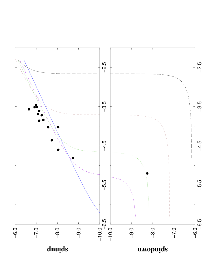
Figure 1: Dependence of period derivative, $\dot{p}$, on the parameter $p^{7/3}f$, $f$– observed flux, for A0535+26. Both axis are in logarithmic scale. Observations (Bildsten et al., 1997) are shown with black dots. Five curves are plotted for different values of the magnetic field. Solid curve: $\mu=1\cdot 10^{30}\,{\rm G}\cdot{\rm cm}^{3}$. Dot-dashed curve: $\mu=5\cdot 10^{30}\,{\rm G}\cdot{\rm cm}^{3}$. Dotted curve: $\mu=10\cdot 10^{30}\,{\rm G}\cdot{\rm cm}^{3}$. Dashed curve: $\mu=30\cdot 10^{30}\,{\rm G}\cdot{\rm cm}^{3}$. Long dashed curve: $\mu=100\cdot 10^{30}\,{\rm G}\cdot{\rm cm}^{3}$. All curves are plotted for the distance $d=2\,{\rm kpc}$.

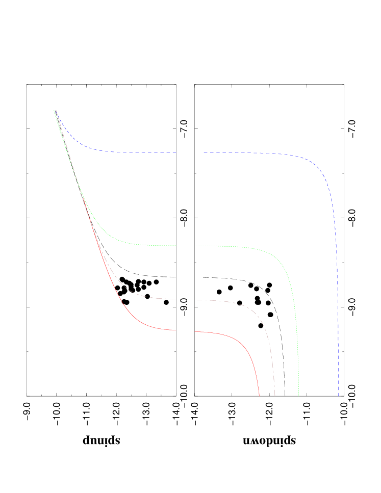
Figure 2: Dependence of period derivative, $\dot{p}$, on the parameter $p^{7/3}f$, $f$– observed flux, for Her X-1. Both axis are in logarithmic scale. Observations (Bildsten et al., 1997) are shown with black dots. Five curves are plotted for different values of the magnetic field. Solid curve: $\mu=0.1\cdot 10^{30}\,{\rm G}\cdot{\rm cm}^{3}$. Dot-dashed curve: $\mu=0.15\cdot 10^{30}\,{\rm G}\cdot{\rm cm}^{3}$. Long dashed curve: $\mu=0.2\cdot 10^{30}\,{\rm G}\cdot{\rm cm}^{3}$. Dotted curve: $\mu=0.3\cdot 10^{30}\,{\rm G}\cdot{\rm cm}^{3}$. Dashed curve: $\mu=1\cdot 10^{30}\,{\rm G}\cdot{\rm cm}^{3}$. All curves are plotted for the distance $d=4\,{\rm kpc}$.

We plot spin-up and spin-down rates as a function of the parameter, which is a combination of the spin period and source’s luminosity. Spin-up and spin-down values derived from the BATSE data (Bildsten et al., 1997) are plotted as black dots, and theoretical curves for different values of the magnetic momentum are also shown. In ideal, the best curve for the magnetic momentum should exist, which fits all observational points. In reality points have some errors, distance to the source in also know with some uncertainty, and simple model of spin-up and spin-down can be only the first approximation. But these estimates of the magnetic momentum are more precise, than the ones obtained with the equilibrium hypothesis.

These estimates can be different from other ones obtained from the equilibrium periods or from a single value of spin-down as can be seen from the table 1.

3 Discussion and conclusions

We made estimates of the magnetic field of NSs in X-ray pulsars. Estimates which were made with an assumption that $p=p_{eq}$ are rather rough. Obtained values depend (except uncertainties connected with the method itself) on unknown parameters of NSs, such as masses, radii, moments of inertia. All of them were accepted to have “standard” values, and of course it is only the first approximation. For example, our estimate for the source GRO 1744-28 is $\mu\sim 10^{30}$ G cm³, and it is smaller than the estimate shown in (Borkus 1998), which is $B\sim(2-5)\cdot 10^{12}$ G (we mark, that the estimate obtained by Joss & Rappaport (1997) is significantly lower than both: Borkus and our estimates). But if one take “non-standard” value for $R$, these estimates of $\mu$ and $B$ can be in good correspondence.

We show several examples in table 3. NSs radii are calculated from the following simple formula:

$$R=\left(2\mu/B\right)^{1/3}.$$

Here $\mu$ are taken from table 1, and values of $B$ are taken from Nagase (1992), Borkus (1998) and Wang (1996). As one can see from the table for several sources measured $B$ are not in correspondence with our calculated $\mu$, and radii of NSs are too big. Mostly these cases are long period wind-fed pulsars like GX 301-2, where formation of temporal reverse disk is possible for the cases of fast spin-down, so there maximum spin-down can be not the best field estimate, and estimates from the equilibrium period for wind-accretion case are in better correspondence with observations. For A 0535+26 our estimate was obtained only from the equilibrium period. And as far as this system is transient it can be far from the equilibrium. We note, that in general existence of high magnetic field in that source, as it comes from our estimates, is confirmed by observations. In the case of 4U 0115+63 errors for maximum spin-down rate are significant, and discrepancy between observed and calculated values can be due to this. We also note, that Ginga was not sensitive enough at the spectral region $\geq 40$ keV, where cyclotron line for $\mu\geq(2-3)\cdot 10^{30}$ G cm³ are situated.

Table 3: Magnetic fields, magnetic momentum and radii

X-RAY	Magnetic	Magnetic	Neutron
PULSAR	momentum	field	star
	(calcul.),	(observ.),	radius,
	$10^{30}$G cm3	$10^{12}$G	km
GRO 1744-28	0.58	$\sim(2-5)$	$\sim(8.3-6.1)$
HER X-1	0.3	3	5.8
4U 0115+63	5.17	1.1	21.1
A 0535+26	101.23	11	26.4
VELA X-1	18.5	2.3	25.2
4U 1535-52	56.4	1.9	39
GX 301-2	281.9	3.5	54.4

In more clear cases (Her X-1, GRO 1744-28), where we are sure, that accretion is of the disk type, our estimates from maximum spin-down are in good correspondence with observations. And we predict for the cases of Be-transients, where disk accretion is working for sure, that in 2S 1417-624, GRO 1948+32, GRO 1008-57, A 1118-616 and 4U 1145-61 observations of cyclotron lines at energies $\geq 100$ keV are possible in future.

Estimates obtained from maximum spin-down rate and estimates obtained with the hypothesis of equilibrium period are in rough correspondence, except sources OAO 1657-415 and 4U 1145-61, where maximum spin-down estimates are significantly higher. It can be an indication, that systems are far from equilibrium (especially in the case of Be-transient 4U 1145-61), or that some additional mechanism of spin-down (outflows, reverse disks, …?) work. In the case of OAO 1657-415 estimate based on maximum spin-down rate can be incorrect similar to GX 301-2 due to the reasons, which were discussed above.

Observations of period and flux variations can be used also for simultaneous determination of magnetic field of a NS and distance to the X-ray source (Popov 1999).

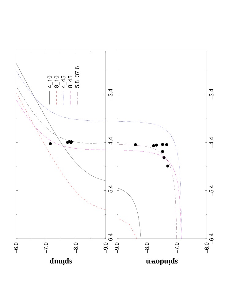
Figure 3: Dependence of period derivative, $\dot{p}$, on the parameter $p^{7/3}f$, $f$– observed flux, for GRO 1008-57. Both axis are in logarithmic scale. Observations (Bildsten et al., 1997) are shown with black dots. Five curves are plotted for disk accretion for different values of distance to the pulsar and NS magnetic momentum. Solid curve: $d=4\,{\rm kpc}$, $\mu=37.6\cdot 10^{30}\,{\rm G}\cdot{\rm cm}^{3}$. Dashed curve: $d=8\,{\rm kpc}$, $\mu=37.6\cdot 10^{30}\,{\rm G}\cdot{\rm cm}^{3}$. Long dashed curve: $d=5.8\,{\rm kpc}$, $\mu=10\cdot 10^{30}\,{\rm G}\cdot{\rm cm}^{3}$. Dot-dashed curve: $d=5.8\,{\rm kpc}$, $\mu=45\cdot 10^{30}\,{\rm G}\cdot{\rm cm}^{3}$. Dotted curve (the best fit): $d=5.8\,{\rm kpc}$, $\mu=37.6\cdot 10^{30}\,{\rm G}\cdot{\rm cm}^{3}$.

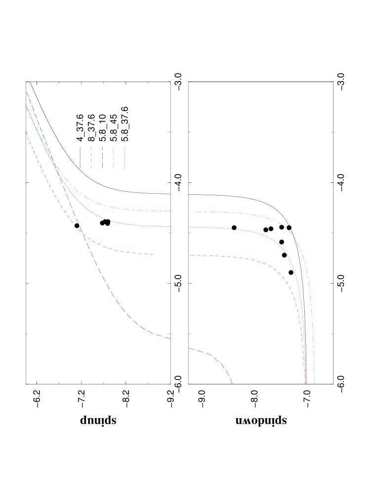
Figure 4: Dependence of period derivative, $\dot{p}$, on the parameter $p^{7/3}f$, $f$– observed flux, for GRO 1008-57. Both are axis in logarithmic scale. Observations (Bildsten et al., 1997) are shown with black dots. Five curves are plotted for disk accretion for different values of distance to the pulsar and NS magnetic momentum. Solid curve: $d=4\,{\rm kpc}$, $\mu=10\cdot 10^{30}\,{\rm G}\cdot{\rm cm}^{3}$. Dashed curve: $d=8\,{\rm kpc}$, $\mu=10\cdot 10^{30}\,{\rm G}\cdot{\rm cm}^{3}$. Long dashed curve: $d=8\,{\rm kpc}$, $\mu=45\cdot 10^{30}\,{\rm G}\cdot{\rm cm}^{3}$. Dot-dashed curve (the best fit): $d=5.8\,{\rm kpc}$, $\mu=37.6\cdot 10^{30}\,{\rm G}\cdot{\rm cm}^{3}$. Dotted curve: $d=4\,{\rm kpc}$, $\mu=45\cdot 10^{30}\,{\rm G}\cdot{\rm cm}^{3}$.

The method is based on several measurements of period derivative, $\dot{p}$, and X-ray pulsar’s flux, $f$. Fitting distance, $d$, and magnetic momentum, $\mu$, one can obtain good correspondence with the observed $p,\,\dot{p}$ and $f$, and that way produce good estimates of distance and magnetic field (see also another way of estimating of these parameters based on the equilibrium period and spin-up measurements applied to GRO1744-28 in (Joss & Rappaport 1997) and (Rappaport & Joss 1997)).

Lets consider only disk accretion due to application of our method to the system, in which most probably accretion is of the disk type. In that case one can write (see Lipunov 1982, 1992):

$$\dot{p}=\frac{4\pi^{2}\mu^{2}}{3\,G\,I\,M}-\sqrt{0.45}\,2^{-1/14}\frac{\mu^{2/7}}{I}\left(GM\right)^{-3/7}\left[p^{7/3}L\right]^{6/7}R^{6/7},$$ (3)

where $L=4\pi d^{2}\cdot f$ – luminosity, $f$ – the observed flux.

So, with some small uncertainty in the equation above we know all parameters ($I$, $M$, $R$ etc.) except $\mu$ and $d$. Fitting observed points with them we can obtain estimates of $\mu$ and $d$. Uncertainties mainly depend on applicability of that simple model.

To illustrate the method, we apply it to the X-ray pulsar GRO J1008-57, discovered by BATSE (Bildsten et al., 1997). It is a $93.5$ s X-ray pulsar, with the BATSE flux about $10^{-9}$ erg  cm^-2 s^-1. A 33 day outburst was observed by BATSE in August 1993. The source was identified with a Be-system with $\sim 135^{d}$ orbital period (Shrader et al. 1999). We use here only 1993 outburst, described in Bildsten et al. (1997).

Bildsten et al. (1997) show flux and frequency history of the source with 1 day integration. In the maximum of the burst errors are rather small, and we neglect them. Points with large errors were not used.

We used standard values of NS parameters: $I=10^{45}\,$ g  cm², momentum of inertia; $R=10\,$ km, NS radius; $M=1.4M_{\odot}$, NS mass.

On figures 3-4 we show observations (as black dots) and calculated curves (in the disk model, see Shrader et al. (1999), who proposed a disk formation during the outbursts, in contrast with Macomb et al. (1994), who proposed wind accretion) on the plane $\dot{p}$ – $p^{7/3}f$, where $f$ – observed flux (logarithms of these quantities are shown). Curves were plotted for different values of the source distance, $d$, and NS magnetic momentum, $\mu$. Spin-up and spin-down rates were obtained from graphs in Bildsten et al. (1997).

The best fit (both for spin-up and spin-down) gives $d\approx 5.8\,{\rm kpc}$ and $\mu\approx 37.6\cdot 10^{30}\,$ G $\cdot$ cm³. It is shown on both figures. The distance is in correspondence with the value in (Shrader et al. 1999), and such field value is not unusual for NSs in general and for X-ray pulsars in particular (see, for example, (Lipunov 1992) and (Bildsten et al. 1997)), and this value of $\mu$ is consistent with maximum spin-down (see table 1). Tests on some other X-ray pulsars with know distances and magnetic fields also showed good results.

The method of distance and field estimates is approximate and depends on several assumptions (type of accretion, specified values of $M,I,R$, etc.). Estimates of $\mu$, for example, can be only in rough correspondence with determinations of magnetic field $B$ with hyrolines, if standard value of the NS radius, $R=10$ km is used (see, for example, the case of Her X-1 in (Lipunov 1992)). When the field and the distance are know with high precision observations of period and flux observations can be used to put limits on the equation of state (see e.g. Schaab & Weigel 1999).

If one uses maximum spin-up, or maximum spin-down values to evaluate parameters of the pulsar, then one can obtain values different from the best fit (they are also shown on the figures): $d\approx 8\,$ kpc, $\mu\approx 37.6\cdot 10^{30}\,$ G$\cdot$ cm³ for maximum spin-up, and two values for maximum spin-down: $d\approx 4\,{\rm kpc}$, $\mu\approx 37.6\cdot 10^{30}\,$ G$\cdot$ cm³ and the one close to our best fit (two similar values of maximum spin-down were observed for different fluxes, but we mark, that formally maximum spin-down corresponds to the values, which are close to our best fit). It can be used as an estimate of the errors of our method: accuracy is about the factor of 2 in distance, and about the same value in magnetic field, as can be seen from the figures.

Determination of magnetic field (and, probably, distance) only from X-ray observations can be very useful in uncertain situations, for example, when only X-ray observations without precise localizations are available.

Acknowledgments

PSB thanks prof. Joss for discussions.

The work was supported by the RFBR (98-02-16801) and the INTAS (96-0315) grants.

References

- [1] Bildsten, L. et al., 1997, ApJ Suppl. 113, p. 367
- [2] Borkus, V.V., 1998, PhD dissertation, Space Research Institute, Moscow
- [3] Joss, P.C., & Rappaport, S., 1997, in IAU Coll. 163 proc., Eds. D.T. Wickramasinghe et al., ASP Conference series, 121, p.289
- [4] Lipunov, V.M., 1992, “Astrophysics of Neutron Stars”, Springer-Verlag
- [5] Lipunov, V.M., 1982, AZh 59, p. 888
- [6] Macomb, D.J., Shrader, C.L., & Schultz, A.B., 1994, ApJ 437, p. 845
- [7] Nagase, F., 1992, in Ginga Memorial Symposium (ISAS Symp. on Astroph.) eds. F.Makino & F.Nagase, p.1
- [8] Popov S.B., 1999, Astr. Astroph. Trans. (in press), astro-ph/9906012
- [9] Rappaport, S, & Joss, P.C., 1997, ApJ 486, p. 435
- [10] Schaab, C., Weigel, M.K., 1999, astro-ph/9904211
- [11] Shrader, C.L., Sutaria, F.K., Singh, K.P., & Macomb, D.J., 1999, ApJ 512, p. 920
- [12] Wang, Y.-M., 1996, ApJ 465, L111