A Far-Infrared Survey of Molecular Cloud Cores

Abstract

We present a catalogue of molecular cloud cores drawn from high latitude, medium opacity clouds, using the all-sky IRAS Sky Survey Atlas (ISSA) images at 60 and 100 $\mu$m. The typical column densities of the cores are $\rm N(H_{2})\sim 3.8\times 10^{21}$cm^-2 and the typical volume densities are $\rm n(H_{2})\sim 2\times 10^{3}$cm^-3. They are therefore significantly less dense than many other samples obtained in other ways. Those cloud cores with IRAS point sources are seen to be already forming stars, but this is found to be only a small fraction of the total number of cores. The fraction of the cores in the protostellar stage is used to estimate the prestellar timescale – the time until the formation of a hydrostatically supported protostellar object. We argue, on the basis of a comparison with other samples, that a trend exists for the prestellar lifetime of a cloud core to decrease with the mean column density and number density of the core. We compare this with model predictions and show that the data are consistent with star formation regulated by the ionisation fraction.

1 Introduction

The denser regions of the interstellar medium are usually known as molecular clouds, and stars form in the very highest density parts of these clouds, which are usually referred to as molecular cloud cores. The process by which material is turned from a molecular cloud core into a star is far from being fully understood, since many complex physical processes are involved (see, for example, Mouschovias 1991, for a review).

The key to understanding the process of star formation appears to lie in the earliest stages of molecular cloud core evolution, since the initial conditions determine much of what subsequently takes place. Many observational studies have been conducted of such dense cores (e.g. Myers & Benson 1983; Myers, Linke & Benson 1983; Clemens & Barvainis 1988; Benson & Myers 1989; Bourke, Hyland & Robinson 1995a), usually starting from an optically selected sample of dark clouds on sky survey plates. In this paper we present a sample of cloud cores selected on the basis of far-infrared optical depth using the IRAS Sky Survey Atlas (ISSA) images (Wheelock et al. 1994), with a view to broadening the range of the physical parameters of cores that have been explored, and hence gaining further insight into the evolution of molecular cloud cores.

The paper is laid out as follows: Section 2 describes the manner in which optical depth maps were constructed from the ISSA data, including technical details such as background subtraction, and goes on to discuss cloud core selection and methodology verification techniques; Section 3 describes the new molecular cloud core catalogue that we have constructed from the data and the associations with previously known molecular clouds and IRAS point sources; Section 4 contrasts the properties of the new catalogue with previous molecular cloud core catalogues and compares the ensemble of mean catalogue properties with the theoretical predictions of models of ionisation-regulated star formation; and Section 5 presents the conclusions of the paper. Readers who are more theoretically inclined may wish to read Sections 3 & 4 before going back to Section 2.

2 Observational details

2.1 Background subtraction

We chose to select the clouds using the IRAS Sky Survey Atlas (ISSA), which is an all-sky set of images at each of the four IRAS wavebands of 12, 25, 60 & 100 $\mu$m (Beichman et al. 1988; Wheelock et al. 1994). However, since we wished to select the coldest, densest clouds, we concentrated on the two longest wavelengths, 60 & 100 $\mu$m. We used these to construct optical depth and temperature maps of the regions of interest, in a similar manner to that adopted by Wood, Myers & Daugherty (1994). These latter authors selected previously known molecular cloud regions, whereas we endeavoured to construct a distinct sample of previously little-studied clouds drawn from the all-sky set of plates. But before optical depth and temperature maps can be made, it is necessary to ensure that all background emission has been removed from the images. This is because in making optical depth and temperature maps, one must take the ratio of emission at two different wavelengths (in this case 60 & 100 $\mu$m). Therefore, any offset at one or other wavelength due to background emission not associated with the object will affect the ratio measurement. The ISSA images have already been fully processed and corrected for most of the Zodiacal background emission, but they still contain extended emission from the Galactic Plane and some residual Zodiacal emission. These are the backgrounds we now address.

Pixel histograms of all the ISSA fields were constructed by binning the pixels in each field into histograms of surface intensity. On examination it was found that some fields’ pixel histograms contained a single peak, some contained double or multiple peaks and some had much more complicated structures. Each field was searched to identify whether the histogram had a peak with a width of less than 2MJysr^-1 (i.e. $\rm\sim$ 10 $\rm\times$ the calibration noise) and at low enough intensity to be consistent with an area of background. Any such peak was taken as evidence of an area of low level emission in the field which can be described as an area of background containing only low level cirrus. A number of the fields were inspected visually. It was found that the pixels in the low level peak of the histogram in each case came from a contiguous, discrete area of the sky, and were not randomly isolated pixels, confirming that this automatic method was indeed finding genuine areas of sky.

A similar method was previously carried out for optical images by Beard, MacGillivray & Thanisch (1990), who showed that histograms of pixels’ intensities contain valuable information about the background regions within the image. In relatively empty areas of the sky the pixel histogram takes the form of a single Gaussian peak whereas in regions densely populated with real sources several further peaks appear in the histogram at higher intensities.

The position of the peak was recorded and used as a measure of the background surface brightness in the field. 272 ISSA fields were identified as having suitable background regions by this technique at 100$\rm\mu$m and 368 were found at 60$\rm\mu$m from a total of 430 for each wavelength. The widths of the low intensity peaks in the pixel histograms were generally at least a factor of two or three larger than the average calibration errors for the field – as estimated from the standard deviation in pixel values from one Hours Confirmed scan (HCON) to the next – indicating the existence of real cirrus structure within the background regions.

To investigate the overall nature of the background, maps which interpolated from region to region of background were constructed. This was done by first recording the values of the pixel histogram low intensity peaks (in MJysr^-1) and recording the central position of the field in which it was found. A simple interpolation technique was devised, somewhat akin to box-car averaging. For every square degree on the celestial sphere the distance to the centre of the nearest few ISSA fields containing a region of background was calculated, to allow averaging. This gives a series of angular displacements to the background regions ($\theta_{\rm{1}},\theta_{2},\theta_{3},\theta_{4},....\theta_{n}$), where:

$$\rm{cos}(\theta_{\rm{i}})=\rm{cos(dec_{i})cos(dec)cos(ra-ra_{i})-sin(dec_{i})sin(dec)}.$$

Here the right ascensions and declinations of the positions to which we wish to interpolate are denoted ra and dec respectively, and the position of each background region is denoted $\rm ra_{i}$ and $\rm dec_{i}$. We then attributed to each position the value of surface brightness:

$$I=\frac{\sum^{\theta_{\rm{i}}<\phi}{\rm cos}\left(\frac{\pi\theta_{{\rm i}}}{\phi}\right)I_{{\rm i}}}{\sum^{\theta_{{\rm i}}<\phi}\rm{cos}\left(\frac{\pi\theta_{{\rm i}}}{\phi}\right)}.$$

This was chosen because it interpolates between positions smoothly, does not produce discontinuities and weights more heavily the nearest background regions, even given the non-uniform spatial sampling of background surface brightness. It essentially involves smoothing by a cosine bell of radius $\phi$. The result of this process was then projected onto a 2d surface with equal area projection to create a map of background brightness for the whole sky.

Fig. 1 shows the map of the background constructed by this technique at 100$\mu$m for $\phi=$ 12 degrees. The plot is an ‘equal area’ projection in Galactic coordinates. The intensity varies smoothly, and increases towards the Galactic Plane indicating that the cirrus intensity within background regions increases towards the Plane. The map contains negative values showing that the Zodiacal background subtraction used in producing the ISSA dataset was liable to over-compensate in some regions. The apparent gap through the centre of the map is due to our having to discard regions of high source confusion in the Galactic Plane, where our Galactic background subtraction did not work due to source confusion.

Figure 1: Interpolated map of 100-$\mu$m background regions. Values range from $-$0.2 to $+$11 MJySr^-1. There is a gap in the data through the map along the Galactic Plane (partly obscured because of the projection), due to a larger number density of clouds near the Galactic plane causing source confusion and thus preventing the background subtraction method from working.

The residual ‘striping’ characteristic of images produced by IRAS was reduced to very low levels in the ISSA images, because of the careful calibration used to produce them. However, the act of ratio-ing two images tends to enhance any striping effects that remain. In some fields this striping was clearly visible, and in some cases dominated the structure of the optical depths maps. These fields were discarded. We selected 60 of the fields used in the interpolation for further study, based on their background regions being clearly identifiable and measurable, and on the quality of the images.

Table 1: List of cloud positions, associations, velocities and distances. In column 4 a superscript indicates that the association is a: (1) dark nebula catalogued by Lynds (1962); (2) bright nebula catalogued by Lynds (1965); (3) molecular cloud identified and mapped in CO by Taylor, Dickman & Scoville (1987); (4) cluster listed by Lang (1992); and (5) molecular cloud identified and mapped in CO by Ramesh (1994).

Cloud	R.A.	Dec.	Associations	Velocity	Distance
Name	(1950)	(1950)	identified	(LSR)/kms-1	(pc)
021A	00h 00m	$-$76∘ 00′	Chameleon	–	200
270A	00h 02m	$+$13∘ 50′	None	–	$\rm<$80
422A	01h 30m	$+$76∘ 30′	Cepheus	–	300–800
423A	02h 10m	$+$75∘ 30′	Cepheus, L1331, LBN2,	$+$3.1$\rightarrow+$3.5	800
			T4863, T4864, Berkeley84
002B	02h 30m	$-$85∘ 00′	Chameleon	–	200
423B	03h 00m	$+$81∘ 20′	Cepheus	–	300–800
411A	04h 15m	$+$64∘ 20′	Cepheus	–	300–800
205A	04h 28m	$+$04∘ 00′	Orion	–	450
050A	07h 26m	$-$48∘ 00′	R425, Merlotte 664	$+$4.8	$\rm<$250
221A	15h 44m	$-$04∘ 00′	$\rm\rho$ Ophiuchus, L134N1	$+$2.6	125
420C	20h 40m	$+$67∘ 00′	Cepheus, L11481, T3793	$+$3.5	300
420B	21h 30m	$+$66∘ 00′	Cepheus, L11761, T3093,	$-$10.8	800
			NGC 71424, NGC 71294
002A	21h 30m	$-$83∘ 00′	Chameleon	–	200
334A	21h 48m	$+$35∘ 30′	None	–	$\rm<$270
422C	22h 00m	$+$77∘ 30′	Cepheus, LBN2,	$-$1.7$\rightarrow+$5.1	300
			T4203,T4283,T4313
422B	22h 45m	$+$73∘ 40′	Cepheus, T4263, T4313	$-$3.7	300

2.2 Colour temperatures

We used the STARLINK data reduction package IRAS90 and, in particular the routine COLTEMP, to create colour temperature and optical depth maps from the ISSA images. We briefly describe the technique here (for further details, see Berry 1993a & b).

The far infrared radiation from a cloud of temperature $\rm T$ emitting a black body spectrum, $\rm B(\nu,T)$, and absorbing $\rm I(\nu,T)d\tau_{\nu}$, at a position in the cloud with an optical depth $\rm\tau_{\nu}$, leads to a flux received by an observer $\rm f(\nu,T)$ given by:

$$\rm f(\nu,T)=\left(1-e^{-\tau_{\nu}}\right)B(\nu,T).$$

Generally $\rm\tau_{\nu}$ is dependent on $\rm\nu$ in such a way (Hildebrand 1983) that:

$$\rm\tau(\nu)=\left(\frac{\nu}{\nu_{c}}\right)^{\beta},$$

where $\rm\beta$ is the dust emissivity index and $\nu_{c}$ is the critical frequency at which the optical depth is unity. Throughout this work we use the value suggested by Hildebrand (1983) of $\rm\beta=1$ at far-infrared wavelengths. These two equations describe a ‘greybody’ spectrum. We assume that the cloud is optically thin at the wavelengths observed – Wood et al. (1994) show that even towards the Galactic Plane this is true. Because $\rm\tau_{\nu}\ll 1$, $\rm 1-e^{-\tau_{\nu}}\sim\tau_{\nu}$ and we therefore use the expression:

$$\rm f(\nu,T)\sim\left(\frac{\nu}{\nu_{c}}\right)B(\nu,T).$$

The IRAS detectors were sensitive over a wide bandpass and there were 4 separate wavebands (i=1, 2, 3, 4 for 12, 25, 60 and 100 $\rm\mu$m respectively) so that the measured flux in waveband i is:

$$\rm f_{i}=\int R_{i}(\nu)\left(\frac{\nu}{\nu_{c}}\right)B(\nu,T)d\nu$$

where $\rm R_{i}(\nu)$ is the spectral response curve for the waveband i receiver (see Beichman et al. 1988).

By taking the ratio of intensities at two wavebands i and j, and using the preceding equation, one can derive

$$\rm\frac{f_{i}}{f_{j}}=\frac{\int R_{i}(\nu)\nu B(\nu,T)d\nu}{\int R_{j}(\nu)\nu B(\nu,T)d\nu}.$$

This value is dependent on T, and the response curves of the receivers. Using the listed response curves in the IRAS Explanatory Supplement (Beichman et al. 1988), one can tabulate $\rm f_{i}/f_{j}$ versus T. In the routine COLTEMP a spline giving T as a function of $\rm f_{i}/f_{j}$ is created by fitting to the tabulated values. For any observations of a cloud at 2 wavelengths one can then estimate the temperature and calculate the critical frequency at which $\rm\tau_{\nu_{c}}=1$:

$$\rm\nu_{c}=\frac{\int R_{i}(\nu)\nu B(\nu,T)d\nu}{f_{i}}.$$

Using this, one can calculate the optical depth of the cloud at another wavelength by using the equation for $\tau$ above. We altered COLTEMP to allow temperatures as low as 10K to be used (the publicly available version only accepts temperatures greater than 30K). In this way, optical depth maps were made of our chosen regions at 100 $\mu$m.

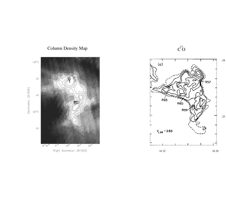
Figure 2: (a) 100-$\mu$m optical depth map of the molecular cloud L1689, produced from the ISSA sky survey plates. Base contour level is 0.8 $\times 10^{-3}$ and the contour interval is 0.3 $\times 10^{-3}$. (b) ¹³CO map of the same field taken from Loren (1989).

2.3 Optical depth maps

The optical depth at 100$\rm\mu$m due to dust along the line of sight is expressible (Hildebrand 1983) as:

$$\tau_{100}=\pi\langle a\rangle^{2}Q_{100}N_{\rm g},$$

where $N_{\rm g}$ is the column density of grains, $\langle a\rangle$ is the average radius of the grains and $Q_{100}$ is the emission efficiency of the dust grains at 100$\rm\mu$m. The mass column density of the grains is then given by:

$$\sigma_{\rm d}=\frac{4}{3}\left(\frac{a\rho}{Q_{100}}\right)\tau_{100},$$

where $\rho$ is the average grain density. The total mass of the dust in a cloud of projected area A is therefore given by:

$$M_{\rm{dust}}=A\langle\sigma_{d}\rangle,$$

where $\langle\sigma_{d}\rangle$ is the mean column density of dust in the cloud. The typical dust-to-gas mass ratio in the local ISM is normally assumed to be approximately 1:100. However it is clear that at 100 $\mu$m a significant fraction of the cold dust in the ISM is not detected, due to temperature and optical depth effects (see e.g. Wood et al. 1994). Hence a simple application of this ratio to these data will underestimate the total mass of gas. Wood et al. (1994) argued that only 1/50 of the total dust is detected at IRAS wavelengths, and used a dust-to-gas ratio of 1:2000 in their analysis. They arrived at this value by using two relations: Firstly they adopted $A_{\rm v}\sim 2\times 10^{4}\times\tau_{100}$ (Langer et al. 1989); and secondly they used $N_{\rm H_{2}}(cm^{-2})\sim 10^{21}\times A_{\rm V}$ (Bohlin, Savage & Drake 1978). We follow Wood et al. (1994) and use a value of 1/2000 in the current study. With a value for $(a\rho/Q_{100})\sim 32$gcm^-1, one obtains the expression for the mass of material in a cloud:

$$M_{cloud}/{\rm M_{\odot}}\sim 1.25\times 10^{-2}\times D^{2}(\rm{pc})\sum_{\rm{cloud}}\tau_{100},$$

where $D$ is the distance to the cloud, and the optical depth of each pixel in the cloud image is summed.

2.4 Cloud selection

Of the resultant optical depth maps, some contained from one to three cloud complexes, varying in size from a few pixels to half a field, while several more were discarded, either due to having very little structure, being too noisy, or having major contamination from residual Zodiacal emission that none of the processing had been able to remove. Some of the clouds were found at the edges of the fields and hence were truncated. ¿From the remaining maps, 17 clouds were selected for further study. The clouds we selected are listed in Table 1: Column 1 lists the name we assigned to each cloud, derived from the ISSA field number in which it was found; Columns 2 & 3 give the approximate position of the centre of the cloud; and the remainder of the table assigns distances, velocities and associations to the clouds we have selected.

It was found that 3 of the clouds were previously identified by Lynds as dark clouds (Lynds 1962), 2 contained Lynds bright nebulae (Lynds 1965), 7 had been identified by other authors (Taylor et al. 1987; Ramesh 1994), who had subsequently measured their CO velocities, and 3 had nearby open cluster associations. Of the 3 open clusters, two have been dated and were found to be old: NGC 7142 is thought to be 4 billion years old; Merlotte 66 is 6 billion years old; in both cases implying that they were probably not linked with the cloud. In addition, comparison with the CO Galactic plane surveys (Dame et al. 1987) revealed that several clouds were associated with known cloud complexes. Only two had no previously published associations. Column 4 of Table 1 lists the known cloud associations.

Unlike molecular maps and surveys, which give the velocity of the clouds and hence give an estimate of the distances, these ISSA selected clouds – like the optically selected clouds of Lynds (1962) – do not have easily derivable distances. Distances were estimated either from velocity and spatial association with the Orion, Cepheus, Chameleon and Ophiuchus complexes, or by estimating an upper limit for distance obtained by assuming the clouds lie in the Galactic Disc – i.e. less than 60 pc away from the Galactic Plane (c.f. Clemens, Sanders & Scoville 1988). Clouds found in Cepheus present a particular problem when one attempts to assign a distance. There are two different complexes along the line of sight: one at approximately 300 pc with a velocity $\rm\sim$ 0 kms^-1; and one in the local spiral arm at approximately 800 pc and with a velocity of $\rm\sim$ $-$12kms^-1 (Grenier et al. 1989). Some of the Cepheus clouds we selected had been sampled with CO observations (Taylor et al. 1987), and the measured velocities revealed the clouds belonged to one or other complex. This revealed that the sample presented here contains clouds from both complexes and hence that the three Cepheus clouds in the sample without CO observations could be at either of the two distances. In total, 11 of the 16 clouds had a single distance assigned to them, 2 had upper limits, and 3 could be at either of 2 distances. Column 5 of Table 1 gives the velocity of the cloud (if previously measured), and column 6 gives the estimated distance.

2.5 The case of L1689

As a cross-check of both the procedure used and the mass estimates derived, we made a map of a previously studied cloud, L1689. Colour temperature and optical depth maps were constructed and the results are presented in Figure 2(a) as a 100-$\mu$m optical depth map of the region. An extended region of high 100-$\mu$m optical depth containing some structure is seen. Figure 2(b) shows a ¹³CO map of the same region taken from Loren (1989). A similar morphology is seen in both maps. The two star-forming cores R57 (alias L1689N), and R59 (alias L1689S) are clearly visible, as is the isolated core R65 (alias L1689B).

At the centre of the cloud there is an apparent ‘hole’ in the optical depth map at the position of the bright point source, IRAS16288, which is a young protostar at the centre of L1689S. Wood et al. (1994) also noted that a bright, point-like source dominating the IRAS emission can cause an apparent hole in the 100-$\mu$m optical depth. They ascribed this to a beam filling factor effect. The right hand side of the above equation for $\tau_{(100)}$ also contains a term for the solid angle of the source, $\Omega$, which has been set equal to 1 in our analysis. For an extended molecular cloud source this is a valid assumption, but it fails when there is a bright point source in the beam. This is the effect we see in the case of IRAS16288.

We calculated the mass of L1689, using the above equation, from the 100-$\mu$m optical depth map in Figure 2(a), and found a value of 448 M_⊙ (assuming a distance of 160 pc). Loren (1989) used the ¹³CO data shown in Figure 2(b), and obtained a value of 566 M_⊙. These two measurements are consistent to within $\pm$20 per cent, which is as accurate as either method can claim, and so we conclude that the technique outlined not only gives accurate qualitative information on the morphology of interstellar clouds, but also appears to provide relatively good quantitative estimates of cloud masses. Nonetheless, we realise that masses derived from 100-$\mu$m optical depths might be underestimated in some cases, if the 100-$\mu$m emission is completely optically thick. In none of the cloud cores that we studied did this appear to be the case.

3 The core catalogue

3.1 Core properties

Figures 3 & 4 show grey-scale images, with isophotal contours overlaid, of nine of our molecular cloud regions. They can be seen to vary in size from 1 to 5 degrees across, and also to vary in complexity and structure. Some residual striping can be seen in two of the fields. However the typical structures associated with molecular clouds can be seen in all of the images – namely cores, filaments and other structures on all scales within the maps. Some of the structure seen in the maps corresponds to previously known molecular clouds, but some of the clouds, and many of the cores, had not been previously catalogued. For example, Figure 3(d), 420B, and Figure 4(d), 423A, both contain a Lynds dark nebula and an open cluster. 423A also contains an HII region and two further catalogued clouds. Some of the regions contain no previous associations – especially those in the southern hemisphere. For a full list of known associations see Table 1 and section 2.4 above.

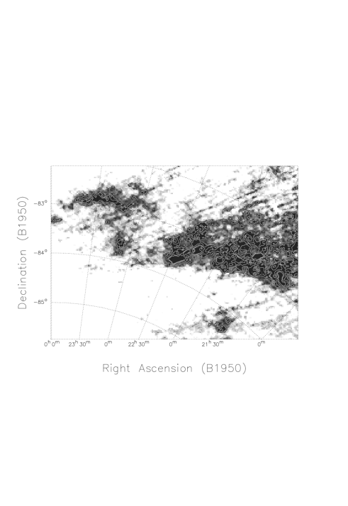
(a)	(b)
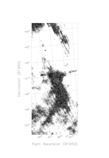
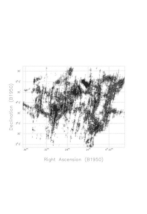
(c)	(e)
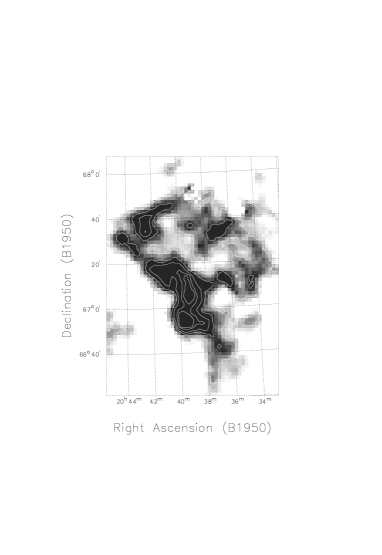
(d)

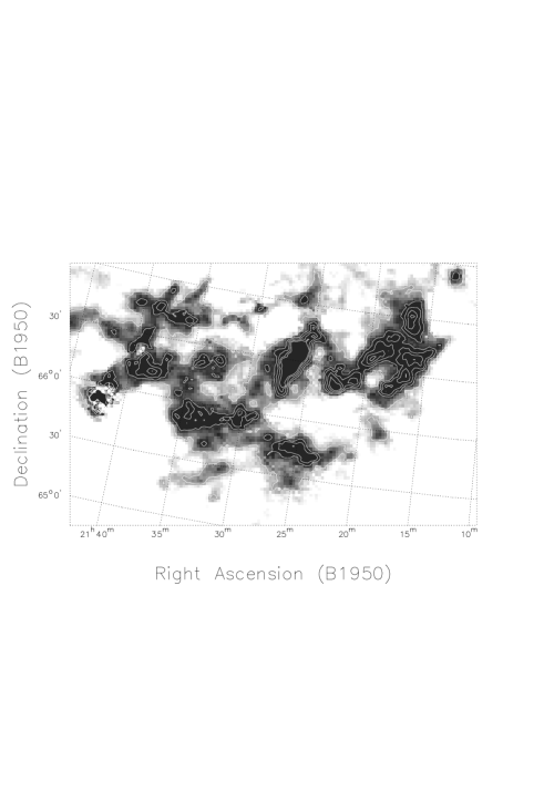
Figure 3: 100-$\mu$m optical depth maps, with contours overlaid, of: (a) 002A; (b) 050A; (c) 205A; (d) 420B; (e) 420C.

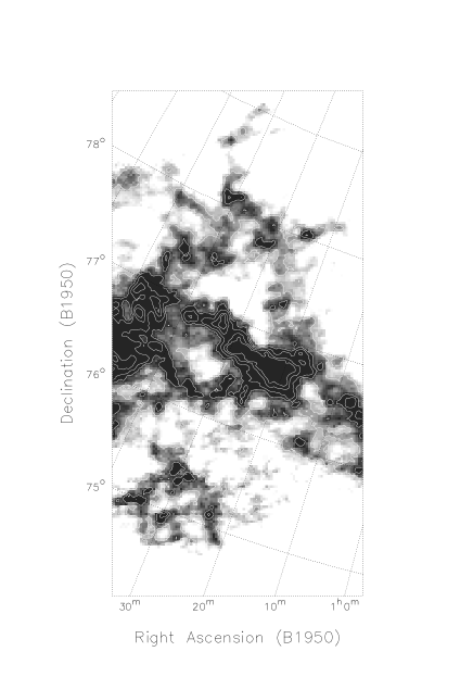
(a)	(b)
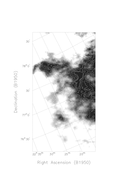
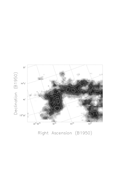
(c)	(d)

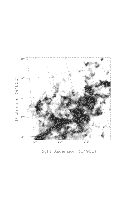
Figure 4: 100-$\mu$m optical depth maps, with contours overlaid, of: (a) 422A; (b) 422C; (c) 422B; (d) 423A

A catalogue of the most opaque regions in each cloud was produced and the maps were examined. The definition of what constitutes a core in a molecular cloud is of necessity somewhat subjective. We chose to define a core as the most opaque 1% of a cloud’s area. This level was chosen to ensure that the area defined as a core was relatively small compared to the cloud, and hence would only include the most dense regions where we would expect star formation to take place. We then calculated the mass of each core.

Table 2: The catalogue of molecular cloud cores, together with their positions, sizes, optical depths, shapes, orientations and masses.

JWT	Cloud	R.A.	Dec.	Temp	Size	$\rm\overline{\tau}$	$\rm\tau_{peak}$	Ellip-	$\overline{\rm r}$	$\theta$	Mass
No.	name	(1950)	(1950)	(K)	(arcmin2)	($\times 10^{-3}$)	($\times 10^{-3}$)	ticity	(pc)	(∘)	(M⊙)
1	270A	00h 03m 03s	$+$13∘ 56′ 30′′	29.2	23.4	0.02	0.018	0.43	$<$0.2	11	$<$2
2	422A	01h 21m 38s	$+$76∘ 41′ 37′′	21.7	105	0.40	0.439	0.43	0.5–1.2	67	300–2100
3	422A	01h 27m 54s	$+$76∘ 44′ 27′′	21.5	45.3	0.38	0.404	0.71	0.3–0.9	68	120–880
4	423A	02h 03m 18s	$+$75∘ 51′ 50′′	20.8	54.7	0.52	0.580	0.68	0.38	71	200
5	423A	02h 20m 46s	$+$75∘ 22′ 54′′	21.4	12.5	0.49	0.505	0.18	0.18	134	44
6	002B	02h 31m 55s	$-$84∘ 56′ 03′′	23.8	21.9	0.12	0.142	0.01	0.16	123	8.3
7	423A	02h 36m 20s	$+$74∘ 57′ 03′′	20.2	26.6	0.55	0.651	0.41	0.26	116	100
8	423B	02h 52m 42s	$+$81∘ 00′ 20′′	22.0	17.2	0.19	0.206	0.69	0.2–0.5	35	20–160
9	423B	03h 15m 55s	$+$81∘ 50′ 15′′	19.8	54.7	0.24	0.411	0.36	0.4–0.9	120	100–690
10	411A	04h 14m 59s	$+$64∘ 19′ 02′′	23.0	92.2	0.37	0.403	0.55	0.5–1.2	167	250–1800
11	411A	04h 17m 01s	$+$64∘ 07′ 09′′	23.3	12.5	0.34	0.352	0.32	0.2–0.5	169	30–220
12	411A	04h 17m 45s	$+$64∘ 14′ 51′′	23.1	29.7	0.35	0.369	0.55	0.3–0.7	22	80–530
13	411A	04h 18m 55s	$+$63∘ 53′ 58′′	22.6	79.7	0.36	0.380	0.66	0.5–1.1	161	200–1500
14	205A	04h 24m 32s	$+$04∘ 54′ 24′′	24.1	136	0.13	0.154	0.58	0.89	38	290
15	205A	04h 25m 23s	$+$04∘ 30′ 14′′	24.6	21.9	0.12	0.132	0.57	0.35	173	44
16	205A	04h 26m 26s	$+$04∘ 30′ 28′′	24.4	57.8	0.12	0.139	0.51	0.58	3	120
17	205A	04h 29m 02s	$+$03∘ 48′ 54′′	24.1	21.9	0.13	0.130	0.52	0.35	168	44
18	205A	04h 30m 18s	$+$03∘ 37′ 46′′	24.2	26.6	0.12	0.128	0.51	0.39	71	53
19	205A	04h 30m 21s	$+$03∘ 18′ 12′′	22.6	31.3	0.13	0.137	0.79	0.43	168	65
20	205A	04h 30m 32s	$+$03∘ 46′ 53′′	24.3	18.8	0.12	0.130	0.51	0.32	178	38
21	050A	07h 26m 05s	$-$48∘ 10′ 15′′	26.3	20.3	0.18	0.188	0.55	$<$0.6	39	$<$200
22	050A	07h 26m 39s	$-$47∘ 54′ 27′′	26.0	34.4	0.18	0.192	0.74	$<$0.8	20	$<$340
23	050A	07h 29m 16s	$-$46∘ 54′ 22′′	25.9	170	0.20	0.278	0.28	$<$1.9	148	$<$1900
24	050A	07h 32m 30s	$-$46∘ 50′ 12′′	25.5	26.6	0.20	0.240	0.30	$<$0.7	97	$<$300
25	221A	15h 30m 12s	$-$03∘ 23′ 34′′	25.0	40.6	0.09	0.101	0.31	1.35	50	4.3
26	221A	15h 39m 03s	$-$03∘ 24′ 15′′	25.1	43.8	0.07	0.079	0.46	0.14	19	4.1
27	221A	15h 40m 36s	$-$03∘ 16′ 05′′	25.0	18.8	0.08	0.077	0.70	0.09	4	1.8
28	221A	15h 43m 25s	$-$03∘ 50′ 38′′	25.4	28.1	0.08	0.081	0.60	0.11	14	2.6
29	221A	15h 44m 21s	$-$03∘ 49′ 22′′	05.6	50.0	0.08	0.086	0.69	0.15	19	4.8
30	021A	18h 03m 10s	$-$75∘ 28′ 48′′	25.6	259	0.06	0.070	0.60	0.55	169	50
31	021A	18h 13m 05s	$-$75∘ 28′ 21′′	25.9	46.9	0.06	0.063	0.63	0.23	174	8.7
32	021A	18h 33m 20s	$-$76∘ 00′ 14′′	25.6	46.9	0.06	0.063	0.11	0.23	141	8.7
33	021A	18h 33m 22s	$-$74∘ 16′ 04′′	25.5	37.5	0.06	0.061	0.36	0.21	11	6.8
34	021A	18h 33m 48s	$-$75∘ 45′ 39′′	25.5	20.3	0.06	0.063	0.61	0.15	173	3.8
35	021A	18h 37m 53s	$-$74∘ 00′ 43′′	25.0	12.5	0.06	0.056	0.66	0.12	157	2.2
36	420C	20h 39m 20s	$+$67∘ 07′ 58′′	19.1	40.6	0.60	0.680	0.62	0.32	175	160
37	420C	20h 39m 37s	$+$66∘ 54′ 51′′	19.0	35.9	0.64	0.761	0.25	0.31	39	170
38	420B	21h 16m 11s	$+$66∘ 39′ 03′′	23.6	29.7	0.35	0.359	0.44	0.35	74	530
39	420B	21h 16m 42s	$+$66∘ 29′ 40′′	23.9	20.3	0.35	0.359	0.20	0.62	130	360
40	420B	21h 16m 43s	$+$66∘ 59′ 26′′	23.3	25.0	0.35	0.369	0.59	0.67	172	450
41	002A	21h 18m 29s	$-$82∘ 49′ 34′′	22.7	59.4	0.15	0.164	0.66	0.26	16	29
42	420B	21h 19m 34s	$+$66∘ 37′ 23′′	23.3	18.8	0.35	0.371	0.62	0.58	120	340
43	420B	21h 22m 38s	$+$66∘ 21′ 22′′	24.5	37.5	0.36	0.393	0.38	0.84	34	690
44	420A	21h 26m 21s	$+$66∘ 30′ 46′′	24.0	177	0.39	0.514	0.65	1.80	149	3600
45	002A	21h 38m 55s	$-$82∘ 45′ 12′′	22.4	54.7	0.16	0.186	0.47	0.25	100	28
46	420B	21h 42m 06s	$+$65∘ 53′ 12′′	43.6	34.4	0.50	1.030	0.34	0.79	62	880
47	334A	21h 46m 35s	$+$35∘ 20′ 01′′	27.5	15.6	0.06	0.063	0.39	$<$0.6	145	$<$60
48	334A	21h 46m 51s	$+$35∘ 00′ 58′′	27.2	48.4	0.06	0.071	0.22	$<$1.0	118	$<$200
49	002A	21h 47m 00s	$-$83∘ 00′ 13′′	22.5	42.2	0.15	0.172	0.62	0.22	95	21
50	334A	21h 47m 31s	$+$35∘ 23′ 19′′	27.3	50.0	0.06	0.065	0.37	$<$1.1	75	$<$200
51	334A	21h 48m 55s	$+$35∘ 46′ 40′′	27.5	15.6	0.06	0.067	0.35	$<$0.6	153	$<$60
52	002A	21h 58m 57s	$-$83∘ 14′ 17′′	23.0	28.1	0.15	0.160	0.23	0.18	83	14
53	002A	21h 59m 28s	$-$83∘ 00′ 02′′	22.4	21.9	0.15	0.156	0.41	0.16	72	11
54	422C	22h 07m 50s	$+$77∘ 22′ 11′′	21.4	25.0	0.30	0.320	0.48	0.25	180	55
55	422C	22h 09m 58s	$+$77∘ 15′ 03′′	21.8	12.5	0.30	0.321	0.61	0.18	170	27
56	002A	22h 15m 50s	$-$83∘ 16′ 45′′	23.2	54.7	0.15	0.170	0.48	0.25	125	27
57	002A	22h 21m 53s	$-$83∘ 23′ 50′′	23.5	21.9	0.15	0.163	0.57	0.16	128	11
58	002A	22h 26m 20s	$-$83∘ 35′ 58′′	23.0	90.6	0.16	0.188	0.59	0.32	98	48
59	422B	22h 41m 33s	$+$73∘ 33′ 48′′	24.1	12.5	0.20	0.207	0.48	0.18	55	18
60	422B	22h 47m 58s	$+$73∘ 18′ 02′′	23.8	15.6	0.20	0.216	0.25	0.20	90	23

Table 3: IRAS point sources associated with the cores in this catalogue, together with their flux densities and other known associations.

JWT	IRAS	Flux densities (Jy)				Other
Number	Association	12$\rm\mu$m	25$\rm\mu$m	60$\rm\mu$m	100 $\rm\mu$m	associations
2	01226+7641	$\rm<$0.58	$\rm<$0.25	$\rm<$0.40	2.50
7	02368+7453	0.44	0.89	0.89	3.21
8	02532+8102	$\rm<$0.25	$\rm<$0.64	$\rm<$0.40	3.57
9	03139+8151	0.33	$\rm<$0.25	$\rm<$0.40	$\rm<$4.99
9	03191+8147	0.29	$\rm<$ 0.25	$\rm<$0.40	$\rm<$5.23	545K01
12	04178+6416	0.67	$\rm<$0.25	$\rm<$0.40	$\rm<$8.18	13118M01
14	04250+0502	$\rm<$0.29	$\rm<$0.26	$\rm<$0.40	2.37
23	07299$-$4644	$\rm<$0.25	$\rm<$0.25	1.05	10.34	MSH 074082
23	07300$-$4653	0.25	$\rm<$0.25	$\rm<$1.37	$\rm<$10.53
23	07305$-$4659	$\rm<$0.41	$\rm<$0.25	0.99	$\rm<$10.25	07305$-$46593
26	15395$-$0330	$\rm<$0.33	$\rm<$0.85	$\rm<$0.40	1.02
34	18333$-$7547	$\rm<$1.33	$\rm<$0.34	$\rm<$0.40	1.47
41	21185$-$8252	$\rm<$0.25	$\rm<$0.25	$\rm<$0.40	2.49
43	21232+6626	$\rm<$2.12	$\rm<$0.25	$\rm<$0.55	9.58
46	21426+6556	$\rm<$0.39	$\rm<$0.27	2.15	$\rm<$21.19
50	21479+3520	1.75	0.51	$\rm<$0.40	$\rm<$1.82	DO 209254
50	21484+3522	$\rm<$0.25	$\rm<$0.25	$\rm<$0.52	2.87
52	21580$-$8316	$\rm<$0.73	$\rm<$0.85	$\rm<$0.40	1.78
58	22278$-$8341	$\rm<$0.36	$\rm<$0.25	$\rm<$0.40	2.56
60	22412+7332	$\rm<$0.25	$\rm<$0.25	$\rm<$0.40	2.98	X2241+7355
60	22422+7333	0.25	$\rm<$0.33	$\rm<$0.40	$\rm<$2.05	RAFGL 29496

Table 2 lists the properties of our new core catalogue. Column 1 lists the new number we have designated for each core in order of Right Ascension. Column 2 lists the cloud in which it is located, following the numbering convention of Table 1. Columns 3 & 4 list the position of the centre of each core. Column 5 lists the derived colour temperature of each core. Column 6 lists the solid angle of each core in square arcmin. Column 7 lists the mean optical depth, and column 8 lists the peak optical depth of the core. Column 9 gives the ellipticity, column 10 lists the mean radius, column 11 lists the position angle (north through east) of the major axis and column 12 lists the mass of each core.

The median 100-$\mu$m optical depth of our 60 cores is 1.9 $\times$ 10^-4, corresponding to a column density of N(H₂) = 3.8 $\times$ 10²¹ cm^-2. The median radius of the cores for which a distance is known is 0.31 pc, with a mean radius of 0.41 pc. The mean is skewed by a small number of large cores, so we prefer to use the median to characterise our sample. The median volume density of the sample is $\sim$2 $\times$ 10³ cm^-3 (the mean volume density is very similar). Hence we see that, by selecting our core sample based on a wavelength of 100 $\mu$m, we have typically selected somewhat lower density cores than many previous surveys of molecular cloud cores (see below). The difference is probably mainly due to our selecting relatively isolated clouds as a result of our constraints on background emission.

3.2 PSC associations

All of the IRAS point sources within the boundaries of each core were located using the Point Source Catalogue (PSC), and are listed in Table 3. The core in which the source is found is noted along with the source flux densities at each IRAS waveband. A superscript in the last column indicates that the IRAS PSC listed a known association for the source: (1) indicates that the source appears in the Smithsonian Astrophysical Observatory Star Catalogue (SAO); (2) represents the catalogue of Ohio State University Radio Sources; (3) is the IRAS Serendipitous Survey Catalogue; (4) is the Dearborn Observatory Catalog of Faint Red Stars; and (5) is the IRAS Small Scale Structure Catalog (Beichman et al. 1988 and references therein).

There are 21 source associations, of which: 11 are detected only at 100 $\mu$m; two are detected only at 60 $\mu$m; with one detected at 60 & 100 $\mu$m, but no shorter wavelengths; five are only detected at 12$\rm\mu$m; one source is detected at 12 & 25 $\mu$m, but not at longer wavelengths; and one source is detected at all four wavebands. The eleven 100-$\mu$m-only sources have upper limits at the shorter wavelengths such that we can say that their spectral energy distributions peak at a wavelength of around 100 $\mu$m or longer. The one source detected at all four wavebands and the source detected at 60 & 100 $\mu$m only, also have rising spectra to longer wavelengths. The other two 60-$\mu$m-only sources are also consistent with having rising spectra. This is the form of spectral energy density we would expect for deeply embedded young stellar objects (YSOs) or protostars. The six sources detected only at the shortest wavelengths have spectra consistent with field stars or other objects. Hence there appear to be 15 PSC sources associated with our 60 cores.

However, some of the PSC associations may still be chance alignments, and in addition the 100-$\mu$m-only sources could be cirrus associated with the clouds rather than embedded YSOs. So two ‘control samples’ were produced by offsetting the core positions by first 2 degrees and then 5 degrees in declination, and selecting the IRAS point sources associated with the new positions. In effect this produces two false populations of cores, one of which is still located in the clouds (the 2-degree offset population), and one of which is located outside of the clouds. This technique was chosen because it was thought that it would introduce the least bias in the estimate of the numbers of associations that were purely chance alignments.

In the control sample produced from a 2-degree displacement we found ten sources. Four were detected only at 100$\rm\mu$m, and five sources were detected at 12 and 25$\rm\mu$m – all of which were brighter at 12$\rm\mu$m than 25$\rm\mu$m. These are thus thought to be main sequence field stars – one had been positively identified as a B star. The one remaining source, which was detected at all wavelengths, was previously catalogued as a galaxy in the Upsalla General Catalogue of Galaxies. In the sample produced at a displacement of 5 degrees there were also ten sources, four of which were 100-$\mu$m-only sources. Six of the sources were detected at both 12 and 25 $\mu$m and were brighter at 12 $\mu$m than 25 $\mu$m, and again are probably field stars.

Hence we find no evidence for a significant difference between the two control samples, either due to the increased displacement, or to the location being inside or outside the clouds. Likewise, we see that the number of foreground stars remains roughly constant both in the control samples and the real sample. Of the remaining 15 PSC associations in the real sample, we conclude that six are probably chance alignments. Of the remainder, up to half may be 100-$\mu$m-only cirrus sources – i.e. the point source might be the cloud core itself (see, for example: Benson & Myers 1989; Reach, Heiles & Koo 1993; Bourke et al. 1995b). Hence we estimate that the number of PSC sources, which are embedded YSOs and are associated with our sample of 60 cores, is five.

4 Comparison with previous core catalogues

4.1 Densities

We can compare our new catalogue of molecular cloud cores with catalogues produced by previous authors using different methods. For example, Myers et al. (1983) surveyed 90 cores in C¹⁸O and ¹³CO. Using these observations they showed that the cores’ C¹⁸O optical depths, as estimated from the ratio of C¹⁸O brightness to ¹³CO brightness, was reasonably tightly distributed around a mean of 0.35 to 0.45. They found that the C¹⁸O column density, $N_{18}$, had a mean of $\sim$ 1.6 $\times$ 10¹⁵ cm^-2. This led them to estimate a typical $N(H_{2})$ column density of $\sim$ 10²² cm^-2.

Clemens & Barvainis (1988) also carried out a survey of molecular cloud cores, and the IRAS images of these cores were studied by Clemens, Yun & Heyer (1991). They found a typical 100-$\mu$m optical depth for their sample of 2.5 $\times$ 10^-4. From this we can estimate a column density of N(H₂) $\sim$ 5.0 $\times$ 10²¹ cm^-2, using the above equations. Wood et al. (1994) carried out a survey of the ISSA data for some known star-forming regions, and produced a catalogue of molecular cloud cores. They found that their cores had a mean column density N(H₂) $\sim$ 4.5 $\times$ 10²¹ cm^-2.

The mean volume density of the cores in each of these surveys can also be estimated. Myers et al. (1983) found a typical volume density in their cores of $n(H_{2})\sim 8\times 10^{3}$ cm^-3. Wood et al. (1994) did not quote a typical volume density but a value can be estimated from their column density if a typical radius for the cores is known. The optimum value to use is complicated by the fact that they defined cores to be areas with visual extinction A_v $>$ 4. This leads to the inclusion of several very large ‘cores’ which we would define as ‘clouds’ (their largest ‘core’ is 329 pc²). This skews their mean to a value much larger than the median. We therefore take the the second quartile boundary of radius, which is $\sim$ 0.5 pc in their sample. This leads to an estimate for the typical number density of 3 $\times$ 10³ cm^-3.

The typical number densities of the Clemens & Barvainis (1988) cores can also be estimated if the typical size of the cores is known. Clemens et al. (1991) claim that the typical radius of the cores is 0.35pc. This was calculated from the mean solid angle of the cores and an assumed distance of 600 pc. However, this distance estimate is somewhat uncertain. It was derived originally by Clemens & Barvainis (1988) from two considerations: firstly that the cores were generally within 12 degrees of the Galactic Plane; and secondly that the cores had LSR velocities of between 0 and 10 kms^-1.

However, Bourke et al. (1995a) argued that, because these cores are seen in extinction against the background stars of the Galactic Plane, the survey is biased towards detecting cores near the Plane. Hence they derive an estimate of the typical distance to the cores of 300 pc. Using this value a typical radius of 0.175pc is derived, and hence a volume density of $n(H_{2})$ $\sim$ 4.8 $\times$ 10³ cm^-3 is calculated for this sample. This is significantly higher than the value quoted by Clemens et al. (1991), mainly due to the different distance assumed, but also partly because we have followed Wood et al. (1994) in calculating column density from 100-$\mu$m optical depth. Lemme et al. (1996) studied a subset of the Clemens & Barvainis (1988) cores and reached a similar conclusion: namely that Clemens et al. (1991) may have underestimated the typical density of the cores in the Clemens & Barvainis (1988) sample.

Bourke et al. (1995b) presented data for two samples of molecular cloud cores: one sample consisted of isolated Bok globules, and the other was a set of cores in more extended clouds. These had mean column densities of 5 $\times$ 10²¹ cm^-2 and 1.6 $\times$ 10²² cm^-2 respectively, and volume densities of 10⁴ cm^-3 and 3 $\times$ 10⁴ cm^-3 respectively. Hence, it can be seen that each of these samples has selected cores with somewhat different properties. We here label the Bourke et al. (1995b) extended sample Bourke(1), and the Bok globule sample Bourke(2). All of the column and volume density estimates have associated errors from a number of causes. These include chiefly the assumed fractional abundance of the different tracers used in each set of observations. We believe that the values quoted are accurate relative to one another to within 20 per cent. Table 4 summarises the mean properties of each of the core samples we have discussed.

Table 4: Summary of mean core properties of previous surveys of molecular cloud cores compared to the present work (JWT). See text for details.

Survey	N(H2)	n(H2)	Protostellar	$\tau$
	$\times$1021	$\times$103	Percentage	$\times$106
	cm-2	cm-3		yrs
Bourke et al.(1)	16	30	61$\pm$10	0.6$\pm$0.15
Myers et al.	12	8	44$\pm$7	1.3$\pm$0.3
Bourke et al.(2)	5.0	10	36$\pm$7	1.7$\pm$0.4
Clemens et al.	5.0	5	27$\pm$4	2.8$\pm$0.6
Wood et al.	4.5	3	23$\pm$3	3.3$\pm$0.6
JWT	3.8	2	9$\pm_{5}^{6}$	10$\pm^{7}_{4}$

4.2 Protostellar content and pre-stellar life-time

A useful parameter in the study of dense cores is the fraction of cores in a given sample that contain protostars or YSOs. This parameter can be used to estimate a mean statistical life-time for the sample. This method was first used by Beichman et al. (1986), who studied the embedded YSOs within the core sample of Myers et al. (1983). They found that 35 cores had IRAS sources meeting the colour selection criteria of embedded YSOs and 43 had no embedded IRAS sources.

This method was also used by Wood et al. (1994) with slightly different selection criteria to discard foreground main sequence stars. They found that 59 out of the 255 cores in their sample had at least one embedded source. We carried out the same test for the cores in the Clemens & Baravainis (1988) sample, and found 65 cores out of 248 have embedded IRAS sources (using the Beichman et al. selection criteria). Bourke et al. (1995b) found that 27 out of their 76 Bok globules had IRAS point sources satisfying the Beichman criteria, while 36 out of 59 of their cores in extended clouds had embedded sources.

Beichman et al. (1986) used the percentage of cores with embedded sources to estimate the lifetime of a core without an embedded YSO by comparing it with the life-time of the embedded YSO phase. They found the life-time of a starless core in this way to be a $\sim\rm 10^{6}$ years. This was based on assumptions relating to the time taken for a star to accrete its total mass, and the time for it to become visible. The uncertainty in this figure is probably about a factor of 2, but this does not affect the following statistical arguments, it would simply move the absolute time-scale as a whole by a factor of 2 (i.e. the absolute values of the vertical axes in Figures 5 and 6 can move up or down by a factor of 2, but the relative positions of the data-points do not move – see below).

Following this method, we here infer a statistical estimate of the pre-stellar lifetime, $\tau$, of the cores studied in each of the samples discussed above. We also make the assumption that in each survey the cores without embedded sources will go on to form protostars in their centres. The cores with embedded sources are assumed to have an average lifetime which is the same in each sample and equal to the embedded YSO time-scale derived by Beichman et al. (1986). This is simply expressible as:

$$\tau=\frac{\mbox{No. of cores without embedded sources}}{\mbox{No. of cores with embedded sources}}\times 10^{6}\mbox{years},$$

where we have taken the lifetime of cores with embedded sources to be $\rm 10^{6}$ years as discussed above (c.f. Ward-Thompson et al. 1994). $\tau$ was calculated for each core sample discussed in section 4.1, and is listed in Table 4.

Figure 5: Plot of inferred pre-stellar lifetime against column density, for each sample discussed in the text. A best-fit exponential of $\tau\propto e^{(10^{22}/N)}$ is also plotted. The reduced chi-squared error on this fit is 1.15.

Figure 6: Plot of the inferred pre-stellar lifetime against volume density, for each sample discussed in the text. A best-fit power-law of $\tau\propto n(H_{2})^{-0.85}$ is plotted as a solid line. The reduced chi-squared error on this fit is 1.0. Functions of $\tau\propto n(H_{2})^{-0.5}$ and $\tau\propto n(H_{2})^{-0.75}$ are also shown, as dotted and dashed lines respectively.

Figure 7: Plot of the column density against volume density, for each sample discussed in the text. A best-fit power-law of $N(H_{2})\propto n(H_{2})^{0.55}$ is plotted as a solid line.

The fraction of cores with embedded sources has random errors, and in the catalogues where the number of cores with embedded sources is large, the 1 $\sigma$ error is simply the square root of the number of cores with embedded sources. The number of cores in the sample presented in this paper has a low number of cores with embedded sources and therefore the uncertainty in the pre-stellar lifetime is dominated by the systematic effects discussed in section 3.2 above. These errors are quoted in Table 4.

It is apparent from Table 4 that the percentage of cores with embedded sources increases with both the mean column density and volume density of the cores. Hence the pre-stellar core lifetime decreases with both column and volume densities. The results are plotted in Figs. 5 & 6.

Figure 5 shows prestellar lifetime versus column density. Each of the points represents one of the data sets listed in Table 4 (B1 signifies Bourke et al.(1) etc.). We fitted a relation to the data of the form $\tau\propto{\rm exp}(10^{22}/N)$. This is shown as a solid line. Figure 6 shows pre-stellar lifetime versus volume density (using the same labelling as in Figure 5). Power law fits to the data points were carried out, and the best-fit was found to be $\tau\propto n(H_{2})^{-0.85\pm 0.15}$, which is shown as a solid line on Figure 6.

Figure 7 plots column density against volume density for each of the core data sets in Table 4, using the same labelling once again. The solid line is a best fit to the data, which is $N(H_{2})\propto n(H_{2})^{0.55\pm 0.13}$. This is of a similar form to the empirical observations usually referred to as Larson’s relations (Larson 1981), although with a somewhat different slope. If we make the assumption that each catalogue is a representitive subset of all star-forming clouds, and the different membership of each subset is simply due to the characteristic density sensitivity of the different tracers used in each study, then we can compare these empirical results with theoretical predictions.

4.3 Comparison with theory

We can compare the dependence of prestellar time-scale on volume density seen here, with the ambipolar diffusion time-scale. However, it must be noted that the densities plotted in Figure 6 are the mean densities for each core sample, volume-averaged over the whole core in each case. They are not the central densities of each core. Hence care must be taken when comparing Figure 6 with ambipolar diffusion models, which usually plot central density versus time-scale.

The ambipolar diffusion time-scale is proportional to the ionisation fraction, $\chi_{i}$. The ionization of the gas can be caused both by ultra violet radiation and cosmic ray ionisation. The canonical form for the relation between cosmic ray ionisation and volume density is usually taken to be a power-law. For example, Mouschovias (1991) uses:

$$\chi_{i}\propto n(H_{2})^{-0.5},$$

which leads to the derivation of the ambipolar diffusion time-scale relative to density of:

$$\tau_{AD}\propto n(H_{2})^{-0.5}.$$

This behavior is plotted as a dotted line in Fig. 6. When additional factors are included (such as chemistry, multiple charge carriers etc.), the volume density has a slightly different influence on recombination rates, and hence ionisation levels. For example, McKee (1989) suggests:

$$\chi_{i}\propto n(H_{2})^{-0.75},$$

leading to:

$$\tau_{AD}\propto n(H_{2})^{-0.75}.$$

This is plotted as a dashed line on Figure 6. It can be seen that the steeper relation is a closer match to the data, and is in fact consistent to within 1 $\sigma$.

The fact that the lowest density point on Figure 6 lies above the best-fit line suggests that at low densities an additional effect may be starting to become significant. This is somewhat tentative, but does have a possible theoretical explanation. For example, McKee (1989) treats ionization and recombination in some detail, and incorporates the role of metals, and UV penetration. He derives an expression for the star formation time-scale which is dependent on both volume density and column density (see his equation 4.5, and his fig. 1). He also shows that UV ionisation affects the star formation timescale, yielding an exponential dependence on column density (McKee equation 5.2) of the form:

$$\tau_{SF}\propto e^{(N_{c}/N)},$$

where $\tau_{SF}$ is the star formation timescale and $N_{c}$ is the critical column density. $\tau_{SF}$ is not the same as the timescale we have plotted in Figure 5, since McKee was referring to the timescale in which an entire molecular cloud is converted to stars and we are considering the timescale for the dense cores within clouds to form stars. Hence his timescales are roughly an order of magnitude greater than ours. However, we may be observing a similar exponential behaviour. The constant in the exponent, $N_{c}$, was derived by McKee to be 1.6 $\times$ 10²² cm^-2 (deduced from his critical extinction estimate of A_V=16), which is consistent, to within the errors, with the value of 1.0 $\times$ 10²² cm^-2 that we derive in Figure 5.

The three parameters of column density, volume density and lifetime are all inter-dependent. Hence Figures 5 & 6 are not independent. Therefore the empirical fits which we have applied to these plots are not strictly separable in the manner we have adopted. However, we used this approach for the sake of clarity and of demonstrating the potential underlying physical processes. From these data we cannot make definitive statements about ionisation mechanisms, but we have shown that the data, not only from our current survey, but also from those earlier surveys that we have discussed above, are all consistent with a picture in which the ionisation levels in molecular cloud cores regulate the star formation timescale.

5 Conclusions

We have presented a catalogue of 60 cores situated in medium opacity molecular clouds, with the aim of broadening the range of physical environments in which star formation has been studied. The catalogued cores typically have lower column densities and volume densities than previously studied samples and a lower fraction of the cores have formed stars. We found a clear trend for cloud cores to form stars more rapidly with increasing volume and column density. We hypothesised that this can be interpreted in the framework of ionisation-regulated star formation.

References

- [Beard et al. 1990] Beard S. M., MacGillivray H. T., Thanisch P. F., 1990, MNRAS, 247, 311
- [Beichmann et al. 1986] Beichman C. A., Myers P. C., Emerson J. P., Harris S., Mathieu J. P., Benson P. J., Jennings R. E., 1986, ApJ, 307, 337
- [Beichmann et al. 1988] Beichman C. A., Neugebauer G., Habing H. J., Clegg P. E., Chester T. J., eds, 1988, Infrared Astronomical Satellite Catalogs and Atlases Explanatory Supplement , NASA RP-1190, Vol 1, US Government Printing Office, Washington DC
- [Benson et al. 1989] Benson P. J., Myers P. C., 1989, ApJS, 71, 89
- [Berrya1993] Berry D. S., 1993a, Starlink User Note 163, Rutherford Appleton Laboratory
- [Berryb1993] Berry D. S., 1993b, IRAS90 Document 29.0, Rutherford Appleton Laboratory
- [Bohlin et al. 1978] Bohlin R. C., Savage B. D., Drake J. F., 1978, ApJ, 224, 132
- [Bourke et al. 1995a] Bourke T. L., Hyland A. R., Robinson G., 1995a, MNRAS, 276, 1052
- [Bourke et al. 1995b] Bourke T. L., Hyland A. R., Robinson G., James S. D., Wright C. M., 1995b, MNRAS, 276, 1067