Scattering and Diffraction in Magnetospheres of Fast Pulsars

Abstract

We apply a theory of wave propagation through a turbulent medium to the scattering of radio waves in pulsar magnetospheres. We find that under conditions of strong density modulation the effects of magnetospheric scintillations in diffractive and refractive regimes may be observable. The most distinctive feature of the magnetospheric scintillations is their independence on frequency. Results based on diffractive scattering due to small scale inhomogeneities give a scattering angle that may be as large as $0.1$ radians, and a typical decorrelation time of $10^{-8}$ seconds. Refractive scattering due to large scale inhomogeneities is also possible, with a typical angle of $10^{-3}$ radians and a correlation time of the order of $10^{-4}$ seconds. Temporal variation in the plasma density may also result in a delay time of the order of $10^{-4}$ seconds. The different scaling of the above quantities with frequency may allow one to distinguish the effects of propagation through a pulsar magnetosphere from the interstellar medium. In particular, we expect that the magnetospheric scintillations are relatively more important for nearby pulsars when observed at high frequencies.

1 Introduction

A number of observational results may possibly be attributed to scattering processes inside pulsar magnetospheres. After most of the present work was completed, the very interesting and convincing results of Sallmen et al. (1999) were published. In this work, the authors found frequency independent (measured at 1.4 and 0.6 GHz) jitter in the arrival time of giant pulses from the Crab (of order $100\mu$sec). In addition, the frequency independence of the spread and the multiplicity of the pulse components with large variations in the pulse broadening times strongly suggests that multiple components of the giant pulses are due to refractive scattering inside the pulsar magnetosphere. Similarly, Hankins & Moffett (1998) found that broadening times for a single giant pulse from the Crab pulsar scale more slowly with frequency than $\lambda^{4}$ (the value predicted if the scattering is due solely to the unmagnetized electron-ion interstellar plasma). Gwinn et al. (1997) determined, using interstellar scintillation, that the size of the Vela pulsar’s radio emission region is about 500 km. This, being of order 1/10 the light cylinder radius, is considerably larger than conventional estimates. Similar results were obtained by Smirnova et al. (1996) and Wolszcan & Cordes (1987) (but see also Cordes, Weisberg & Boriakoff 1983). Gwinn et al. (1999) found that pulsar 0437-471 shows frequency independent scintillations with bandwidth 4 MHz at several observing frequencies below 1 GHz. Kramer et al. (1997) found that intensity fluctuations at very high frequencies (30 GHz) are considerably enhanced if extrapolated from from observations at lower frequencies. Kramer et al. (1999) found frequency-dependent changes in one of the pulse components of the msec pulsar PSR J1022+1001 these take place on a characteristic frequency scale of 8 MHz at the frequency 1410 MHz. With a dispersion measure of only 10 ${\rm\,pc/cm^{3}}$, this pulsar is probably too close to show diffractive interstellar scintillations with such bandwidth. Citing the authors of the above reference ”a propagation effect in the pulsar magnetosphere might be still the most probable explanation for the observed phenomena.”

Simple models for the interstellar medium fail to fully explain the scattering properties of nearby pulsars. This scattering is enhanced, relative to that extrapolated from more distant pulsars (Sutton 1971), and shows stronger refractive effects (Gupta et al. 1994, Bhat et al. 1999, Rickett et al. 1999). The proposition by Hajivasiliou (1992) and Bhat et al. (1998) that the excess scattering of nearby pulsars lies at the surface the Local Bubble was criticized by Britton et al. (1998) who found strong upper limits on the angular broadening of 5 nearby pulsars, and found that these sizes were inconsistent with both a uniform medium and scattering at the surface of the Local Bubble. Through the examination of the angular and temporal broadening of nearby pulsars, Britton et al. (1998) also concluded that the scattering material of nearby pulsars lies near the pulsars, and is moving in the same general direction as the pulsars. Rickett et al. (1999) found that scattering material for PSR 0809$+$74 probably lies close to the pulsar, using a technique based on the time scale of scintillation, although it could lie much closer if its velocity were aligned with that of the pulsar. Scattering in pulsar magnetospheres could contribute to interstellar scattering and eliminate the necessity of postulating a different, nearby, scattering medium. Taken together, these results compelled us to investigate the scattering of radio waves inside the pulsar magnetosphere.

A theory of interstellar scattering is well developed and has been successfully applied to explain various effects observed in pulsars (Blandford & Narayan 1985,Lee and Jokipii 1975a,b,c, Rickett 1977). In this work we will study the effects of scattering and diffraction inside the pulsar magnetosphere. Strong magnetic fields present in pulsar magnetospheres and the unusual electrodynamics of the one-dimensional electron-positron plasma both change the familiar effects of scattering and refraction in plasma. The unusual features of scattering in such plasma may allow separation from the interstellar scattering and will serve as a tool to probe the structure of the magnetosphere itself.

A large variety of wave-plasma interactions, including scattering and diffraction, may be described in terms of the variation of the refractive index of a medium. A superstrong magnetic field plays a dominant role in defining the electron-photon interactions at small energies. Typically, the frequency of the observed radio waves is much less that the cyclotron frequency $\omega\ll\omega_{B}$. In this limit, the strong magnetic field suppresses the wave-plasma interaction by $(\omega/\omega_{B})^{2}$ (the Thompson cross-section is smaller by this ratio compared to an unmagnetized medium). For such frequencies the refractive index of strongly magnetized pair plasma for escaping electromagnetic modes is approximately

$$n^{2}-1\approx{\omega_{p}^{2}\over\omega_{B}^{2}},$$ (1)

which is fundamentally different from the case of unmagnetized electron-ion plasma (where $n^{2}-1=-{\omega_{p}^{2}\over\omega^{2}}$). In Eq. (1) $\omega_{p}$ is the plasma frequency, $\omega_{B}$ is the nonrelativistic cyclotron frequency. Equation (1) assumes that the plasma is stationary in the pulsar frame. On the open field lines, the pair plasma is moving with a larger streaming Lorentz factor $\gamma$. Then, the refractive index for waves propagating at comparatively large angles to the magnetic field $\theta\gg 1/\gamma_{p}$ is (see appendix A)

$$n^{2}-1\approx{\gamma_{p}\omega_{p}^{2}\over\omega_{B}^{2}}\equiv\delta.$$ (2)

Thus, the large Lorentz factor of the moving plasma effectively enhances the wave-plasma interaction on the open field lines.

Parameter $\delta$ is the key to the scattering and diffraction effects in the pulsar magnetosphere. An important fact is that $\delta$ does not strongly depend on our assumptions about the density and the streaming Lorentz factors of the plasma. To see this, we normalize the density of the secondary plasma to the density of the beam, $\omega_{p}^{2}=\lambda_{M}\omega_{GJ}^{2}=2\lambda_{M}\omega_{B}\Omega$, where $\lambda_{M}$ is a multiplicity factor, and use the fact that the energy in the plasma is approximately equal to the energy in the beam, $\gamma_{p}\lambda_{M}\approx\gamma_{b}$. We find then

$$\delta={2\gamma_{b}\Omega\over\omega_{B}}$$ (3)

Theoretical estimates (e.g. Arons 1983) of the beam’s Lorentz factor give $\gamma_{b}\approx 10^{6-7}$. This value is determined by the condition of vacuum breakdown due to pair production, and depends mostly on the structure of the magnetic field (radii of curvature) in the acceleration zone. In the first approximation, $\gamma_{b}$ may be considered a constant for all the pulsars, regardless of their spin period or surface magnetic field. Then for a conservative estimate $\gamma_{b}\approx 5\times\,10^{5}$, parameter $\delta$ near the light cylinder (where scattering is most important - see below) is

$$\delta=3\times\,10^{-4}\left({P\over 0.1{\rm\,sec}}\right)^{2}\,\left({B_{NS}\over 10^{12}{\rm\,Gs}}\right)^{-1}.$$ (4)

This is a comparatively large value. For example, a fluctuation of the order of unity in the relative density inside the magnetosphere will induce time delays of the order of $\delta P\approx 30\mu{\rm\,sec}$; this is a small value if compared with the total interstellar time delay for typical pulsars, but it is comparable to the relative dispersive interstellar time delay between the frequencies separated by 1 GHz.

Parameter $\delta$, which determines refractive properties of the medium, is negligible deep inside the pulsar magnetosphere, but increases with the distance from the neutron star as $\propto r^{3}$. Thus, the strongest nonresonant wave-plasma interactions occur in the outer regions of pulsar magnetospheres (near the light cylinder). This allows for a considerable simplification when considering scattering and diffraction effects since one can adopt a ”thin screen” approximation. We assume that emission is generated deep in the pulsar magnetosphere and then scattered in a thin screen located near the light cylinder with a typical thickness $D\approx 0.1R_{LC}$.

The physical picture of the disturbances that we have in mind consists of small scale and large scale turbulence. The former is excited possibly by microscopic plasma turbulence or nonlinear plasma interactions (like Langmiur collapse or modulation instability), while the latter is mostly due to the temporal and spatial modulation of the outflowing pair plasma at the moment of its creation. We suppose that the typical sizes of the small scale inhomogeneities should be comparable to tens of Debye radii $a_{\rm\,min}\approx 10\times\,r_{D}=10\omega_{p}/v_{T}\approx 3\times\,10^{2}{\rm\,cm}$ ($v_{T}$ is a typical thermal velocity, $r_{D}$ is a Debye radius); while typical sizes of the large scale inhomogeneities are of the order of a tenth of the light cylinder radius $a_{\rm\,max}\approx 0.1R_{LC}=5\times\,10^{7}{\rm\,cm}$. As we will show later, the small scale inhomogeneities will contribute to diffractive scattering, while larger scale inhomogeneities will contribute to refractive scattering.

Since a detailed spectrum of the density perturbations inside the pulsar magnetosphere is presently not known, we will also make estimates for the power law spectrum extending from smallest scales $a_{min}$ to largest scales $a_{max}$. Relating these two qualitatively different effects by a simple power law may be less justified here than for the case of interplanetary and interstellar media. However, it allows for a consistent treatment of refractive and diffractive effects and, permits the use of well developed methods. We expect the results to depend qualitatively on either the inner or the outer scales and only weakly on the particular choice of the power law index $\alpha$.

Another difference from the case of interstellar scattering worth mentioning here is that while plasma in the pulsar magnetospheres is one dimensional, we still expect the small and large scale turbulence to be three dimensional. At large scales this is an obvious consequence of the temporal and spatial modulation of the outflowing pair plasma; at small scales, the excitation of transverse turbulence (modulating densities of plasma across the magnetic field) is thought to be as effective as excitation of longitudinal turbulence (e.g., Weatherall).

Contradictory estimates exist regarding the development of small scale turbulence in the pulsar plasma. The primary source of this turbulence is usually associated with electrostatic instabilities which may not have enough time to develop (Melrose 1995 ). On the other hand, the existence of the large scale density fluctuations is certain. If the small scale turbulence, which is responsible for the diffractive scattering (see below), does not develop, then our estimates for refractive-type effects will still be valid .

There is an important unresolved problem which may affects the results of this work. Electromagnetic waves should be absorbed in the outer parts of the magnetosphere at the cyclotron resonance:

$$\omega\approx{\omega_{B}/\gamma_{p}}.$$ (5)

This resonance occurs in the outer regions at

$$r\approx 3\times\,10^{8}{\rm\,cm}\left({\nu\over 10^{9}}\right)^{-1/3}.\left({\gamma_{p}\over 100}\right)^{-1/3}\,\left({B_{NS}\over 10^{12}}\right)^{-1/3}$$ (6)

Nonetheless, radiation avoids being absorbed.

In addition, dispersion relation Eq. (2) is valid only for $\omega\ll{\omega_{B}/\gamma_{p}}$. In order to avoid the absorption at the cyclotron resonance, we limit our considerations to fast pulsars with periods $P$

$$P<0.13\,{\rm\,sec}\,\left({\nu\over 10^{9}}\right)^{-1/3}\left({\gamma_{p}\over 100}\right)^{-1/3}\,\left({B_{NS}\over 10^{12}}\right)^{-1/3}.$$ (7)

For numerical estimates, we will use pulsars with a period $P=0.1\,{\rm\,sec}$, surface magnetic field $B_{\rm\,NS}=10^{12}{\rm\,G}$, plasma frequency on the open field lines $\omega_{p}^{2}=2\,\lambda_{M}\,\Omega\,\omega_{B}$, multiplicity factor $\lambda_{M}=5\times\,10^{3}$ and a streaming Lorentz factor $\gamma_{p}=100$. Then at the light cylinder radius $R_{LC}=5\times\,10^{8}{\rm\,cm}$, the parameter for both open and closed field lines is $\delta\approx 3\times\,10^{-4}$.

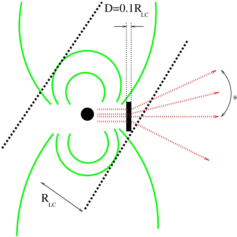
Figure 1: The emission is generated deep in the pulsar magnetosphere and then scattered in a thin screen located near the light cylinder with a typical thickness $D\approx 0.1R_{LC}$.

2 Order of magnitude estimates

2.1 Diffractive and refractive scattering in the case of inhomogeneities of two scales

Consider a screen of thickness $D$, with irregularities of typical size $a$. A variation in the refractive index $\Delta n$ extending over a length $a$ induces a change in the phase of a wave by $\delta\phi\approx\omega a\Delta n/c$. Using dispersion relation Eq. (2) the variation in the refractive index may be written as

$$\Delta n\approx 4\pi r_{e}c^{2}\gamma_{p}\Delta N_{e}/\omega_{B}^{2}=\delta\Delta n_{e}$$ (8)

where $r_{e}=e^{2}/mc^{2}$ is the classical radius of an electron, and we have normalized density perturbations as $\Delta n_{e}\equiv\Delta N_{e}/N_{e}$. The phase shift relative to a vacuum-propagating wave after propagating the distance $a$, is

$$\delta\phi\approx 2\pi\delta\,\Delta n_{e}\,{a\over\lambda}\propto\lambda^{-1}.$$ (9)

The inverse wavelength dependence of the phase shift highlights the important point: scattering becomes stronger at high frequencies. This is opposite to the scattering trend by ISM.

A ray passing through the whole screen encounters $D/a$ randomly distributed irregularities; therefore, the difference between the phases of rays separated laterally by more than $a$ is

$$\Delta\phi\approx 2\pi\left({D\over a}\right)^{1/2}\delta\phi=\left({D\over a}\right)^{1/2}\delta\,\Delta n_{e}\,{a\over\lambda}.$$ (10)

The form of the scattered image will depend on whether the scattering is weak (when $\delta\phi\ll\pi$) or strong (when $\delta\phi\gg\pi$). The angular spectrum of waves has two limiting cases:

$$\theta_{s}={\lambda\over a},\mbox{ $\Delta\phi\ll\pi$}\mbox{}$$

$$\theta_{s}={\Delta\phi\over 2\pi}{\lambda\over a},\mbox{ $\Delta\phi\gg\pi$ }$$ (11)

In the case of weak scattering, we see the initial wave and a thin halo around the mostly unscattered wave. In this limit, the transverse dimension of the correlation function, $\rho_{c}=\lambda/\theta_{c}$, is equal to the size of inhomogeneities. In the case of strong scattering, most of the energy of the initial wave has been transformed into a scattered component. The transverse dimension of the correlation function becomes smaller: $\rho_{c}\approx a/\Delta\phi$.

In the case of scattering inside the pulsar magnetosphere, the typical phase delay $\Delta\phi$ is larger than $\pi$ (see below) - this implies that scattering occurs in the strong regime. The rays are typically scattered by the angle

$$\theta_{\rm\,scat}\approx{\Delta\phi\over 2\pi}{\lambda\over a}=\left({D\over a}\right)^{1/2}\delta\,\Delta n_{e}.$$ (12)

The two types of inhomogeneities that should be present inside the pulsar magnetosphere will produce qualitatively different effects: small scale inhomogeneities will produce diffractive scattering, while large scale inhomogeneities will produce refractive scattering. To see this, we recall (e.g. Prokhorov et al. 1975) that strong scattering may occur in refractive, diffractive or mixed regimes. Separation into refractive and diffractive effects is based on the observation that the geometric optics limit becomes unsuitable for distances larger than

$$L_{\rm\,cr}={a_{\rm\,min}^{2}\over\lambda}.$$ (13)

For larger distances, the diffractive pattern due to the refractive inhomogeneities becomes important regardless of the small size of the diffraction angle. Thus we can identify two scattering regimes (i) diffractive, where the inhomogeneities are seen mostly in the Fraunhofer zone and (ii) refractive, where the inhomogeneities produce fluctuations in the index of refraction and can be described by the geometrical optics approximation. The two limits are separated by the size of the first Fresnel zone, $r_{f}=\sqrt{\lambda R_{\rm\,LC}}\approx 10^{5}{\rm\,cm}$. Inhomogeneities with a size less than the size of the first Fresnel zone contribute to diffractive scintillations, while those with a size larger than the first Fresnel zone contribute to refractive scintillations.

For diffractive scattering, Eq. (12) is an estimate of the the apparent angular size of the source seen through the screen. Numerically for $D\approx 0.1R_{LC}$, $a=a_{\rm\,min}$ and under the most optimistic assumption of relative density fluctuations of the order of unity $\Delta n_{e}\approx 1$, we find:

$$\theta_{\rm\,D}\approx 0.1{\rm rad}.$$ (14)

This implies that large angle scattering is possible in the outer regions of pulsar magnetospheres. The observed profiles are then the convolution of the ”initial” window function (determined by the emission conditions at lower radii) with diffractive scattering.

We would like to reiterate here the the estimate of the scattering angle in Eq. (14)assumes that all the power in the density fluctuations is concentrated at one diffractive scale and that the turbulence is strong $<\Delta N_{e}>\approx N_{e}$. Given the total power in fluctuation (e.g. $<\Delta n_{e}>^{2}\approx 1$), the assumption of a power law spectrum of density fluctuations removes some power from small scales and reduces the diffractive scattering angle (see Sec. 2.2). On the other hand, parameter $\delta$ increases with period of the pulsar - in the longer period pulsars it will be larger than we assumed.

The diffractive image will be focused and defocused by the refractive fluctuations with a scale $\approx\theta_{D}R_{LC}\approx a_{max}$. A typical refractive scattering angle is

$$\theta_{\rm\,R}\approx\delta=4\times\,10^{-3}.$$ (15)

Refractive effects will induce ”jitter” in the arrival times of the pulses and a temporal correlation in the intensities with a typical scale $\tau_{R}=\theta_{\rm\,R}P=4\times\,10^{-4}{\rm\,sec}$. Both of these effects will be independent of frequency, and increasing with the period of the pulsar.

As we have already mentioned, a necessary requirement to allow the separation of scintillations into diffractive and refractive branches is that the scattering should be strong (the total phase shift (Eq. (10)) is much larger than $\pi$). Using our simple estimates (Eq. (10)) for a medium with given size inhomogeneities, we find that this condition is satisfied for

$$a_{\rm\,min}>{\lambda^{2}\over D\delta^{2}}=2\times\,10^{2}{\rm\,cm}.$$ (16)

Alternatively, for a given size of inhomogeneities $a>a_{\rm\,min}$ the scattering is strong for

$$\lambda<\lambda{\rm\,max}=\sqrt{aD}\delta\approx\left\{\begin{array}[]{ll}30\,{\rm\,cm}&\mbox{ for $a=a_{\rm\,min}$}\\ 10^{5}\,{\rm\,cm}&\mbox{ for $a=a_{\rm\,max}$}\end{array}\right.$$ (17)

A very important point is that this is a limitation of the wavelength from above: scattering is stronger for shorter wavelengths. This is in sharp contrast to the scattering in the interstellar medium, where the strength of the scattering increases at low frequencies.

For the typical wavelength of observations $\lambda=30{\rm\,cm}$, both refractive and diffractive scattering occurs in a strong scattering regime with the total phase change (Eq. 10):

$$\Delta\phi\approx\left\{\begin{array}[]{ll}1&\mbox{ diffractive}\\ 100&\mbox{ refractive}\end{array}\right.$$ (18)

Diffractive scattering is, though, only mildly strong. In comparison, in the ISM the small scale scintillations are saturated, while large scale are not.

The diffractive scattering angle $\theta_{D}$ will determine the lateral size $\sigma$ of the scatter-broadened spot:

$$\sigma\approx\theta_{D}R_{LC}\approx 5\times\,10^{7}{\rm\,cm}$$ (19)

Interestingly, this is very similar to the size of the emission region of the Vela pulsar found using interstellar scintillations (Gwinn et al.1997) and consistent with other measurements of the emission sizes (Smirnova et al. 1996).

Propagation of radiation through scattering media will also introduce temporal smearing of the pulse and related frequency decorrelation. Usually, these effects are due to the combination of three independent contributions (Lee and Jokipii 1975b ): (i) dispersive decorrelation effects arising from the nonzero $\partial^{2}\omega/\partial k^{2}$ (which for sufficiently narrow receiver bandwidth effectively lead to a decrease in decorrelation bandwidth) (ii) diffractive decorrelation due to small scale scattering and (iii) refractive decorrelation due to the different transit times along the different ray paths. An important difference in our case is that dispersive decorrelation effects will be absent, since the waves are nondispersive.

The extra path length introduced by strong diffractive scattering is $1/2\theta_{\rm\,scat}^{2}R_{LC}$. This will contribute to time delay and pulse broadening of the order

$$\tau_{D}={R_{LC}\theta_{\rm D}^{2}\over 2c}=\approx 10^{-4}{\rm\,sec},$$ (20)

(with corresponding decorrelation bandwidth $\Delta\nu_{D}=2\times 10^{3}{\rm\,Hz}$). There is also a comparable group delay due to changing group velocity

$$\Delta t_{group}\approx\delta\frac{D}{c}\approx 10^{-5}{\rm\,sec}.$$ (21)

In addition, the motion of the scatter-broadened spot due to both the rotation of the pulsar and the motion of scattering material inside the pulsar magnetosphere will produce refractive-type focusing and defocusing. The size of the diffraction pattern at Earth will be $b\approx\lambda/\theta_{diff}\approx 10^{15}{\rm\,cm}$, where

$$\theta_{diff}\approx\theta_{D}{R_{LC}\over L}\approx 10^{-13}$$ (22)

is the visible size of the scattering spot ($L$ is the distance of a pulsar to the Earth). The motion of this diffraction pattern due to the rotation of the pulsar will produce variations on a diffractive scintillations decorrelation time scale of

$$\tau_{diff}={b\over L}P\approx{\lambda\over c\theta_{D}}\approx 10^{-8}{\rm\,sec},$$ (23)

with associated decorrelation bandwidth

$$\Delta\nu_{diff}={1\over 2\pi\tau_{diff}}\approx 10^{7}{\rm\,Hz}.$$ (24)

Motion of the scattering material inside the pulsar magnetosphere will produce diffractive scintillations on the same time scale.

In addition the motion of the scattering disk of the size $\sigma$ will produce refractive type variations with a typical time scale

$$\tau_{R}\approx\theta_{R}P=10^{-4}{\rm\,sec}$$ (25)

and refractive decorrelation bandwidth

$$\Delta\nu_{R}\approx 2\times 10^{3}{\rm Hz}$$ (26)

2.2 Motion of plasma

Plasma in the pulsar magnetosphere is moving along the magnetic field lines with relativistic velocities. This motion will affect the observed intensities in two ways: (i) motion of the inhomogeneities will produce temporal variations in the observed flux, (ii) we may expect to see aberration effects like relativistic contraction of the density inhomogeneities along the direction of motion which will produce a diffractive picture that is not circularly. The observed scattered image of the point source will have an elongated form with a ratio of axis $\approx\gamma_{\perp}$ ($\gamma_{\perp}$ is a Lorentz factor of the motion in the plane of the sky - the parallel component of the perturbation’s wave vector does not affect the scattering. For matter moving at an angle of about 45 degrees to the line of sight, we can estimate $\gamma_{\perp}\approx\sqrt{\gamma}=10$. Thus, the image should be strongly elongated in the direction perpendicular to the direction of motion of matter. This effect, if resolved, will help to determine an absolute position of the rotation axis of the pulsar on the sky.

To see how abberations appears in the general approach we note that for the case of frozen inhomogeneities, both motion of the plasma and relativistic contruction can be treated in the same systematic approach if we transform the distribution function of the index fluctuations from the plasma rest frame $P_{k}\delta(\omega)$ to the laboratory frame.

The Lorentz transformation of the power spectrum of density inhomogeneities $P^{l}$, is related to the untransformed power spectrum $P$ as

$$P^{l}({k^{l}}_{\parallel},k_{\perp})=P(\gamma k_{\parallel},k_{\perp}).$$ (27)

while the transformed correlation function of the power spectrum $\psi^{l}$ is related to the untransformed correlation function $\psi$ as

$$\psi^{l}({r^{l}}_{\parallel},r_{\perp})=\psi({r_{\parallel}\over\gamma},r_{\perp}).$$ (28)

(here the sign ${\parallel}$ denotes componets along the velocity of the medium). Using these relations it is easy to see that the relativistically moving medium is similar to a medium with anisotropic turbulence.

2.3 Power-law distribution of inhomogeneities

In turbulent media, it is common for the spectrum of the density perturbation to be a power law. Below we give order-of-magnitude estimates for this case (assuming that power law index $\alpha$ is less than four).

There are some substantial differences between scattering by a screen with one scale and a power law. First, the correlation function of intensity fluctuations for the one-scale screen has scales of the order of the size of the inhomogeneities of the phase screen; while for the power law, the correlation function of intensity fluctuations has scales of the order of the Fresnel zone $\sqrt{\lambda R_{LC}}$. Secondly, the one-size screen can give strong focusing in the limit of scintillations (e.g., caustics can form if no diffractive size inhomogeneities are present); while in the case of the power-law screen, scintillation only approaches unity.

The power law of density perturbations may extend from smallest scales $a_{min}=1/q_{1}\approx 5\times\,10^{2}{\rm\,cm}$ to largest scales $a_{max}=1/q_{0}\approx 5\times\,10^{7}{\rm\,cm}$. To estimate the scattering for the power law spectrum of density perturbations $\Psi_{N_{e}}\propto k^{-\alpha}$, we note that the typical mean square density fluctuation due to waves with $k\approx 1/a$ is $\delta N_{e}^{2}\approx N_{e}^{2}(q_{0}/k)^{\alpha-3}$. The total phase delay due to the fluctuations on the scale $a\approx 1/k$ for strong turbulence $\delta N_{e}^{2}/N_{e}^{2}\approx 1$ is then

$$\Delta\phi=\sqrt{{D\over a}}\sqrt{\delta n^{2}}\delta{a\over\lambda}\approx D^{1/2}q_{0}^{(\alpha-3)/2}a^{{\alpha-2\over 2}}\lambda^{-1}\delta.$$ (29)

The mean scattering angle

$$\theta=\Delta\phi{\lambda\over a}=\sqrt{{D\over a}}\sqrt{\delta n^{2}}\delta\approx D^{1/2}q_{0}^{(\alpha-3)/2}\delta a^{{\alpha-4\over 2}}$$ (30)

is independent of frequency. For $\alpha<4$ (which includes the Kolmogorov spectrum $\alpha=11/3$), the scattering is mostly due to the small scale density fluctuations; while for $\alpha>4$, scattering is mostly due to the large scale refractive density fluctuations. The mean scattering angle (Eq.30) generally has only a weak dependence on the size ($a^{-1/6}$ for the Kolmogorov spectrum). This suggests that the contribution from all scales may not be negligible.

Estimates of the strength of the scintillations can be made for a power law distribution. The minimum scale that contributes to the strong scattering at a given frequency is (assuming $\alpha>2$)

$$a_{\rm\,strong}={1\over q_{0}}\left({q_{0}\over D}\right)^{{1\over\alpha-2}}\lambda^{{2\over\alpha-2}}\approx 2{\rm\,cm}.$$ (31)

Moreover, for a given size $a$ the scattering is strong for

$$\lambda<\lambda{\rm\,max}=\sqrt{{D\over q_{0}}}\left(q_{0}a\right)^{{\alpha-2\over 2}}\approx 20a^{5\over 6}{\rm\,cm},$$ (32)

where we assumed $q_{0}\approx 1/D$ and $\alpha=11/3$.

2.4 Finite size of the emission region

Untill now we neglected the finite size of the source in assuming that the initial unscattered wave corresponds to a plane wave. Finite size of the emission region may quench the scintillations.

The criterion for scintillation to be quenched depends on whether the scintillation is weak or strong and whether the scintillation is refractive or diffractive. Weak scintillation, or strong refractive scintillation, will take place if the angular size of the source seen from the observer is less than the angular size of the scattering disk. For scattering very near the source (as magnetospheric scattering for a pulsar), scattering will take place if the linear size of the source is less than the linear size of the scattering disk. Strong diffractive scintillation will take place if the linear size of the source is smaller than the linear resolution of the scattering disk, seen as a lens. This can be expressed by requiring that the size of the source be less than $\lambda/\theta_{S}$, where $\theta_{S}$ is the angular size of the scattering disk, seen from the source. For scattering at the light cylinder right near the source, $\theta_{S}$ is the same as the total scattering angle $\theta_{D}$. Note that even if diffractive scintillation is quenched by finite size ofthe source, diffractive scattering will still lead to angular broadening.

For a 0.1-sec pulsar, the light cylinder radius is $R_{L}=5\times\,10^{8}$ cm, the emission region size of the order of the polar cap radius $R_{PC}\sim 1$ km refractive scintillation will take place if the scattering angle is greater than $\Delta W\approx 2R_{PC}/R_{L}\approx 5\times\,10^{-4}$ rad. Diffractive scintillation will take place if the scattering angle is less than $\lambda/(2R_{PC})$. For 30 cm-wavelength observations of a 1-km polar cap, the required scattering angle of $3\times\,10^{-4}$ rad.

For a msec pulsar, with the similar emission region size and cap and the light cylinder radius is $R_{L}=3\times\,10^{7}$ cm ($P=$5-msec) the refractive scintillation will take place if the scattering angle is greater than $10^{-2}$ rad while the limits on diffractive scattering will be the same as for 0.1-sec pulsar.

Quenching by finite source size may also serve as an additional test to distinguish interstellar and magnetospheric diffraction: the latter should be more prominent in pulsars with narrow pulses.

2.5 Millisecond Pulsars

In this work we limited ourselves to fast rotating pulsars, for which the refractive index for radio wave propagation is independent of frequency. In slower rotating pulsars, the magnetic field near the light cylinder (adjusted for the relativistic motion of plasma) falls below the wave frequency; the plasma modes then have a ”normal” dispersion (refractive index $\propto 1-\omega_{p}^{2}/\omega^{2}$). Scattering effects by such a plasma may change the simple frequency dependence (or independence) of the predicted effects.

We expect that our order-of-magnitude estimates of scattering effects will hold for millisecond pulsars as well. Near the light cylinder, the parameter $\delta$ (Eq. 4) is of comparable order for both millisecond pulsars and normal pulsars. The width of the scattering screen, which in millisecond pulsars occupies the whole magnetosphere, is also of the same order $\approx 5\times\,10^{7}{\rm\,cm}$. The Fresnel radius is slightly smaller: $r_{f}=\sqrt{R_{LC}\lambda}\approx 4\times\,10^{4}{\rm\,cm}$. Quenching of diffractive scintillation may be more of a problem for millisecond pulsars, however, since they have larger emission beams.

3 General considerations

In this section we give general formulae for the scattering of electromagnetic waves by turbulent media within the pulsar magnetosphere. If the smallest size of the inhomogeneities is much larger than the wavelength, we can use the scalar wave equation to describe the wave scattering. Using the size of the first Fresnel zone $r_{F}=\sqrt{\lambda R_{\rm\,LC}}\approx 10^{5}{\rm\,cm}$ for comparison purposes, we see that scattering by the inhomogeneities larger than $r_{F}$ occur in the geometric optics limit, while scattering by the inhomogeneities smaller than $r_{F}$ occur in the Fraunhofer limit. To avoid considering two models of scattering (as did Blandford & Narayan) we employ the Markov approximation, which is valid for short wavelengths satisfying both i) $\lambda\ll a_{\min}$ ($a_{\min}$ is the smallest scale of inhomogeneities) and ii) $\lambda\ll l_{c}$ where $l_{c}$ is the radius of coherence of the field (see below) (Rytov et al.).

In the Markov approximation, the medium is assumed to be a collection of uncorrelated scattering phase screens - the correlation function of the refractive index fluctuations $\psi({\bf r})$ is assumed to be delta correlated along the line of propagation:

$$\psi_{n}({\bf r})=<u({\bf r}_{\perp},z)u^{\ast}({\bf r}_{\perp}^{\prime},z^{\prime})>=A({\bf r}_{\perp}-{\bf r}_{\perp}^{\prime})\delta(z-z^{\prime})$$ (33)

(Rytov et al.). Then $A({\bf r}_{\perp})$ - the two dimensional correlation function - is related to the refractive index fluctuations as

$$A({\bf r}_{\perp})=\int dz\psi_{n}({\bf r}_{\perp},z)=\int J_{0}(k_{\perp}r_{\perp})P_{n}({\bf k}_{\perp},0){d^{2}{\bf k}_{\perp}\over(2\pi)^{2}}.$$ (34)

The physical meaning of the correlation function is that $z={\lambda^{2}\over A(0)}$ gives a length at which most of the energy of the wave is converted from ordered component into fluctuating. Related to the correlation function is the two dimensional structure function of the refractive index fluctuations for a homogeneous medium:

$$D({\bf r}_{\perp})=2\left(A(0)-A({\bf r}_{\perp})\right)={1\over\pi}\int_{0}^{\infty}\left(1-J_{0}(k_{\perp}r_{\perp})\right)P_{n}(k_{\perp},0)k_{\perp}dk_{\perp}.$$ (35)

The scattering properties of the pulsar magnetosphere are well approximated by that of an equivalent screen. The equivalent screen structure function of the phase fluctuations for a homogeneous medium is

$$D_{S}({\bf r}_{\perp})={D\over\lambda^{2}}D({\bf r}_{\perp})={8\pi^{2}r_{e}^{2}r_{L}^{4}D\gamma_{p}^{2}\over\lambda^{2}}\int_{q_{1}}^{q_{0}}dk_{\perp}k_{\perp}\left(1-J_{0}(r_{\perp}k_{\perp})\right)\Psi_{\Delta N_{e}}(k_{perp}),$$ (36)

where $r_{L}=c/\omega_{B}$ is the Larmor radius.

The normalized correlation function of the wave field $u({\bf r}_{\perp},z)$ immediately after the screen is

$$\Gamma(r_{\perp},z)=\exp\{-D({\bf r}_{\perp})_{S}\}=<u({\bf r}_{\perp},z)u^{\ast}({\bf r}_{\perp},z)>=\exp\{-{z\over\lambda^{2}}D({\bf r}_{\perp})\}.$$ (37)

One can define several scales associated with the phase structure function $D({\bf r}_{\perp})_{S}$: (i) the typical scale of $D(\rho_{c})_{S}=1$ determines the transverse coherence radius $\rho_{c}$, so that the fields separated laterally by less that $\rho_{c}$ are strongly correlated; (ii) a longitudinal length $z_{c}={\lambda^{2}\over D({\bf r}_{\perp})}$ which determines the minimal distance at which the Markov approximation is applicable; (iii) second (and larger) derivatives at zero displacement determine the typical small scale ($r_{\perp}\ll a_{\rm\,min}$) behavior of the phase structure function

$$a_{2}^{-2}={\partial^{2}D(0)_{S}\over\partial r_{\perp}^{2}}.$$ (38)

For larger scale inhomogeneities (such that $a_{\rm\,min}\gg\lambda$), the transverse correlation radius after the screen is equal to the transverse correlation radius on the screen $l_{\perp}=\rho_{c}$; while the longitudinal correlation length is $l_{\parallel}=\rho_{c}^{2}/\lambda\gg\rho_{c}$.

3.1 Power law distribution

We consider the power spectrum of the density perturbations $\Psi_{N_{e}}({\bf k})$ as the initial quantity for our approach. It is related to the the power spectrum of the refractive index perturbations $P_{n}({\bf k})$ as

$$P_{n}({\bf k})=\delta^{2}{\Psi_{N_{e}}({\bf k})\over N_{e}^{2}}.$$ (39)

We will use the following approximation for the refractive index perturbations:

$$P_{n}({\bf k})={B\exp\{-k^{2}/q_{1}^{2}\}\over(1+k^{2}/q_{0}^{2})^{\alpha/2}},$$ (40)

where the outer scale is $1/q_{0}=a_{\rm\,max}\approx D$, and the inner scale is $1/q_{1}=a_{\rm\,min}$. The dependence of the various effects on the power law index is complicated. In what follows we assume that $3<\alpha<4$ (which includes the Kolmogorov value of $\alpha=11/3$).

The correlation function of the refractive index perturbations is

$$\psi(r)=\int e^{i{\bf k\cdot r}}P_{q}d^{3}q\approx\left\{\begin{array}[]{ll}(q_{0}r)^{\alpha}r^{-3}B=(q_{0}r)^{\alpha-3}\delta^{2}&\mbox{ $\frac{1}{q_{1}}<r<\frac{1}{q_{0}}$ }\\ (\frac{q_{0}}{q})^{\alpha}B=q_{1}^{5-\alpha}q_{0}^{\alpha-3}r^{2}\delta^{2}&\mbox{ $r\ll\frac{1}{q_{1}}$}\end{array}\right.$$ (41)

The normalization of $P_{n}$ is determined by the the mean square of the refractive index perturbations:

$$\left\langle\varepsilon^{2}\right\rangle=\int d^{3}{\bf k}P_{n}$$ (42)

$$B=\frac{8\pi^{3/2}\Gamma(\frac{\alpha}{2})}{q_{0}^{3}\Gamma(\frac{\alpha}{2}-\frac{3}{2})}\delta^{2}\left(\frac{\left\langle\delta N_{e}^{2}\right\rangle}{N_{e}^{2}}\right)$$ (43)

To normalize the spectrum of the refractive index perturbations, we assume that the turbulence is strong, i.e., the mean square of the relative density perturbations is of the order of unity:

$${\left\langle\delta N_{e}^{2}\right\rangle\over N_{e}^{2}}=1.$$ (44)

Then, we obtain the following expression for the coefficient B:

$$B=\frac{8\pi^{3/2}\Gamma(\frac{\alpha}{2})}{q_{0}^{3}\Gamma(\frac{\alpha}{2}-\frac{3}{2})}\delta^{2}\sim 1.3\times\,10^{18}{\rm\,cm}^{3}.$$ (45)

For $\alpha=11/3,$ $q_{0}=10^{-8}cm^{-1},$ and $\delta=3\times\,10^{-4},$

Note, that for the chosen range of $\alpha$, the normalization of the turbulent spectrum depends only on the outer scale; in this case, the increase of the power spectrum at small wave vectors outweighs the large phase volume at large wave vectors.

For the power spectrum (Eq. 40) for distances much larger than the inner scale $r_{\perp}\gg 1/q_{1}$, the 2-D correlation function is

$$A({\bf r}_{\perp})={Bq_{0}^{2}(q_{0}r_{\perp})^{\mu}K_{\mu}(q_{0}r_{\perp})\over 2^{\mu+1}\pi\Gamma(\mu+1)},$$ (46)

where $\mu=\alpha/2-1$.

For distances smaller than the outer scale $r_{\perp}\ll q_{0}$ and for $\alpha<4$ this simplifies to

$$A({\bf r}_{\perp})={Bq_{0}^{2}\over 2\pi(\alpha-2)}\left(1-{\Gamma(2-\alpha/2)\over\Gamma(\alpha/2)}\left({q_{0}r_{\perp}\over 2}\right)^{\alpha-2}\right)\mbox{ $1/q_{1}\ll r_{\perp}\ll 1/q_{0}$ and $\alpha<4$}.$$ (47)

Using the definition of $B$ (Eq. 45) we find

$$A(r_{\perp})=\frac{4\sqrt{\pi}}{q_{0}}\delta^{2}\frac{\Gamma(\frac{\alpha}{2})}{\Gamma(\frac{\alpha}{2}-\frac{3}{2})}\frac{1}{\alpha-2}\left[1-\frac{\Gamma(2-\alpha/2)}{\Gamma(\alpha/2)}(\frac{q_{0}\rho}{2})^{\alpha-2}\right]\approx 10{\rm\,cm}.$$ (48)

On the other hand, for scales much smaller than the inner scale $r_{\perp}\ll 1/q_{1}$

$$A({\bf r}_{\perp})_{r_{\perp}\ll 1/q_{1}}={Bq_{0}^{2}\over 2\pi(\alpha-2)}\left(1-{1\over 4}q_{0}^{\alpha-2}q_{1}^{4-\alpha}r_{\perp}^{2}(\alpha-2)\Gamma({4-\alpha\over 2})\right)\mbox{ $r_{\perp}\ll 1/q_{1}$}.$$ (49)

So that the typical length scale $z_{A}$ associated with A is

$$z_{A}=\frac{\lambda^{2}}{A(0)}\sim 100cm.$$

The 2-D structure functions of the index fluctuations are

$$D(r_{\perp})={Bq_{0}^{2}\over\pi(\alpha-2)}{\Gamma(2-\alpha/2)\over\Gamma(\alpha/2)}\left({q_{0}r_{\perp}\over 2}\right)^{\alpha-2} 1/q_{1}\ll r_{\perp}$$ (50)

$$D(r_{\perp})={Bq_{0}^{2}\over 4\pi}\Gamma({4-\alpha\over 2})q_{0}^{\alpha-2}q_{1}^{4-\alpha}r_{\perp}^{2} r_{\perp}\ll 1/q_{1}$$

Using the definition of B (Eq. 45) we find for $1/q_{1}\ll r_{\perp}$

$$D(r_{\perp})=\frac{8\sqrt{\pi}}{q_{0}}\frac{\delta^{2}}{\alpha-2}\frac{\Gamma(2-\alpha/2)}{\Gamma(\frac{\alpha}{2}-\frac{3}{2})}\left(\frac{q_{0}\rho}{2}\right)^{\alpha-2}.$$ (51)

The condition $D(r_{\perp})_{S}=1$ defines $\rho_{c}$, the correlation length:

$$\rho_{c}={2\over q_{0}}\left[{8\pi\over BDk^{2}q_{0}^{2}}{\Gamma(\alpha/2)(\alpha-2)\over\Gamma(2-\alpha/2)}\right]^{1/(\alpha-2)}=\frac{2}{q_{0}}\left[\frac{q_{0}}{Dk^{2}\sqrt{\pi}}\frac{\alpha-2}{\delta^{2}}\frac{\Gamma(\frac{\alpha}{2}-\frac{3}{2})}{\Gamma(2-\frac{\alpha}{2})}\right]^{\frac{1}{\alpha-2}}\approx 10^{4}{\rm\,cm}.$$ (52)

Note that in our case the correlation length is smaller than the Fresnel radius ${\rho_{c}\leq r_{f}}$.

The other characteristic scale of $D_{S}$, which determines the small scale $r_{\perp}\ll 1/q_{1}$ behavior, is

$${1\over a_{2}^{2}}=\left|{\partial D_{S}(r_{\perp})\over\partial r_{\perp}^{2}}\right|_{r_{\perp}=0}\approx\left({8\pi\over Bq_{1}^{4}\Gamma({4-\alpha\over 2})}\right)^{1/2}\left({q_{1}\over q_{0}}\right)^{\alpha/2}\approx 10^{6}{\rm\,cm}.$$ (53)

Thus the structure function is almost constant for $r_{\perp}\ll 1/q_{1}$ and has a typical correlation length $\rho_{c}$ given by Eq. (52).

As the waves propagate through a turbulent medium, the angular spectrum will tend to become Gaussian. This occurs at (Lee & Jokipi 1975a)

$$z_{G}={\lambda^{2}\over Bq_{1}^{2}}\left({q_{1}\over q_{0}}\right)^{\alpha}{\Gamma(3-\alpha/2)\over\Gamma(2-\alpha/2)}\approx 10^{9}{\rm\,cm}.$$ (54)

This is much larger than the radius of the light cylinder, so that the angular spectrum does not become Gaussian in our considerations.

There are several typical scattering angles associated with the power law distribution. First, there is the mean square angle:

$$\left\langle\theta^{2}\right\rangle=-{1\over 2}D\nabla_{\perp}^{2}D(r_{\perp})\left|{}_{r_{\perp}=0}\right|={BDq_{0}^{2}\over 4\pi}\Gamma({4-\alpha\over 2})q_{0}^{\alpha-2}q_{1}^{4-\alpha}\sim 6\times\,10^{-6}.$$ (55)

This is much smaller than the diffractive angle given in Eq. (14) for small scale inhomogeneities and is comparable to the refractive scattering angle Eq. (15) obtained using simpler considerations. As we have mentioned, this is expected because our order-of-magnitude estimates for inhomogeneities dominated by small scales assumed that all of the power is concentrated at the diffractive scale. For the case of the power law, the power in the density perturbations is attenuated by the large phase space of long wavelengths refractive-type perturbations.

The other characteristic angle $\theta_{c}$, which determines the typical width of the angular power spectrum for a power law distribution, is defined by the correlation radius $\theta_{c}={1\over k\rho_{c}}$:

$$\theta_{c}={q_{0}\over 2k}{\left[{BDk^{2}q_{0}^{2}\over 8\pi}{\Gamma(2-\alpha/2)\over\Gamma(\alpha/2)(\alpha-2)}\right]}^{1/(\alpha-2)}={q_{0}\over 2k}{\left[{\sqrt{\pi}Dk^{2}{\delta}^{2}\over q_{0}(\alpha-2)}{\Gamma(2-\alpha/2)\over\Gamma({\alpha-3\over 2})}\right]}^{1/(\alpha-2)}\approx 10^{-3},\mbox{ if $1/q_{1}\ll\rho_{c}1/q_{0}$}.$$ (56)

The ratio of the two angles is

$${\theta_{c}^{2}\over\left\langle\theta^{2}\right\rangle}\approx 0.2\mbox{ for $\alpha\approx 4$}$$ (57)

The two angles scale differently with frequency: $\left\langle\theta^{2}\right\rangle$ is independent of frequency, while $\theta_{c}\propto\nu^{{2\over\alpha-2}}$ ($\propto\nu^{1/5}$ for Kolmogorov spectrum). They are just different measures of the angular spectrum; in principle, the two angles can serve to distinguish between Gaussian and power-law spectra of the density perturbations.

3.2 Temporal broadening and Decorrelation

In the absence of dispersive decorrelation, the intensity of the initial delta-pulse is a convolution of refractive and diffractive contributions only:

$$P(z,t)=P_{D}(z,t)\ast P_{R}(z,t).$$ (58)

The refractive Green function $P_{R}(z,t)$ has a symmetrical Gausian form (Lee and Jokipii 1975b ):

$$P_{R}(z,t)={2ck^{2}\over\sqrt{2\pi A(0)D}}\exp\left({-2c^{2}k^{4}(t-z/v_{g})^{2}\over A(0)D}\right)$$ (59)

with characteristic refractive decorrelation time and bandwidth

$$\tau_{R}=\frac{1}{c}\left[\frac{A(0)D}{2}\right]^{1/2}=10^{-5}{\rm\,sec}\mbox{}$$

$$\Delta\nu_{R}={1\over 2\pi\tau_{R}}\approx 2\times\,10^{4}{\rm\,Hz}$$ (60)

The diffractive Green function $P_{D}(z,t)$ has an approximately exponential shape with a characteristic time of

$$\tau_{D}={D\theta_{c}^{2}\over 2c}\approx 10^{-7}{\rm\,sec},$$ (61)

and an associated decorrelation bandwidth of

$$\Delta\nu_{D}={1\over 2\pi\tau_{D}}\approx 2\times\,10^{6}{\rm\,Hz}.$$ (62)

In case of power law spectrum the size of the diffraction pattern at Earth will be $b\approx\lambda/\theta_{diff}\approx 10^{17}{\rm\,cm}$, where

$$\theta_{diff}\approx\theta_{D}{R_{LC}\over L}\approx 10^{-15}$$ (63)

is the visible size of the scattering spot. The motion of this diffraction pattern due to the rotation of the pulsar will produce variations on a diffractive scintillations decorrelation time scale of

$$\tau_{diff}={b\over L}P\approx{\lambda\over c\theta_{D}}\approx 10^{-10}{\rm\,sec},$$ (64)

with associated decorrelation bandwidth

$$\Delta\nu_{diff}={1\over 2\pi\tau_{diff}}\approx 10^{9}{\rm\,Hz}.$$ (65)

These is a very larger decorrelation bandwidth. It is of the order of the observed frequency. Generally, the typical diffractive effects are weaker in the case of the power law spectrum of density inhomogeneities. This is due to the fact that in case of power law spectrum there is smaller power on the diffractive scales (given the fixed total power) than in the case of single size inhomogeneities. This makes the diffractive effects due to power law weaker and less likely to be observed.

There though a possibility to distinguish power law from other types of density spectra. In case of power law distribution of inhomogeneities both $\tau_{D}$ and $\delta\nu_{D}$ are weakly dependent on the frequency ($\tau_{D}\propto\nu^{2/5}$) because of the frequency dependence of $\theta_{c}$. In contrast, if we have a Gaussian spectrum of density fluctuations, $\tau_{R}$ would be proportional to $<\theta>$ and independent of frequency. This again may possibly serve as a test for the type of power spectra: for a Gaussian spectrum, the diffractive decorrelation time $\tau_{D}$ should be independent of frequency; while for a power law spectrum, $\tau_{D}\propto\nu^{2(4-\alpha)/(2-\alpha)}$.

3.3 Correlations of intensities

The correlation function of the wave intensities does not have an analytical representation (Rytov et al.). Asymptotic expressions are possible in the cases of weak or very strong scintillations. The division between these two limits is based on whether $D(r_{f})_{S}$ - the value of the structure function of the phase correlations at the first Fresnel zone - is $\ll 1$ or $\gg 1$. This may be cast in the form of the ratio of the first Fresnel zone to the coherence radius $\sqrt{\lambda D}/\rho_{c}$: scintillations are weak for $\sqrt{\lambda D}/\rho_{c}\ll 1$, and strong in the opposite case.

It is easy to see using Eqns (50) that in our case $D(r_{f})_{S}\approx 100\gg 1$. In this limit the scintillation becomes saturated with the scintillation index reaching 1. According to Prokhorov et al. 1975, there are two regimes for the spectrum of scintillations, separated by $q^{\ast}\approx 1/\sqrt{\lambda D}D(r_{f})_{S}^{{\alpha-1\over\alpha(\alpha+1)}}\approx 1/r_{f}$ (this is equivalent to the separation between diffractive and refractive scintillation). For $q\ll q^{\ast}\approx 1/r_{f}$ the modulations are weak, and the modulation spectrum is $\propto q^{4}$ (Prokhorov et al. 1975 (4.40)) - these are diffractive scintillations. For $q\gg q^{\ast}$ - refractive scintillations - modulations are strong and saturated: $m_{z}\approx 1$.

If $D(r_{f})_{S}>1$ the scintillation index is (Prokhorov et al. 1975)

$$m^{2}\approx 1+{\rm\,C}D(r_{f})_{S}^{-{2\over\alpha(2-\alpha)}}$$ (66)

where ${\rm\,C}$ is of the order of unity.

Thus we conclude that strong saturated refractive scintillations are possible inside pulsar magnetosphere.

4 Observational Tests

Here we summarize the predicted characteristics of the scattering inside the pulsar magnetosphere:

diffractive scattering angle	$10^{-1}$
diffractive scattering time	$10^{-4}{\rm\,sec}$
diffractive decorrelation time	$10^{-8}{\rm\,sec}$
refractive scattering angle	$10^{-3}$
refractive decorrelation time	$10^{-4}{\rm\,sec}$
arrival time variations	$10^{-4}{\rm\,sec}$

All these quantities are independent of frequency, but the strength of scattering increases with frequency. This frequency dependence of the strength of scattering is opposite to the interstellar propagation effects (which are weakest at larger frequencies). Thus the weak magnetospheric effects should be most prominent at high frequencies in nearby pulsars.

In conclusion we discuss some observational facts that may possibly be attributed to magnetospheric scattering and propose future or follow up experiments to test the theory.

Some of the propagation effects have possibly been observed. The most interesting and decisive (in our opinion) observations of Sallmen et al. (1999) became known to us when most of the present work was completed. Two results of this work strongly support our theory: the frequency independent jitter in the arrival time, of the order $100\mu$sec; and the frequency independent spread of the multiple components of the giant pulses, of tens of $\mu$sec, with various scattering times also of the order of tens of $\mu$sec. Using our results, these observations imply that the multiple structure of pulses is due to the multipath propagation inside the pulsar magnetosphere: it is frequency independent, but different rays propagate different lengths, aquiring a range of scattering times.

Other observations that can be interpreted in favor of magnetospheric propagation include the following. Large sizes of the emission region(Gwinn et al. 1997, Smirnova et al. 1996 and Cordes et al. 1983) may be due to diffractive scattering. Increase in the temporal broadening time $\tau_{D}\approx 10^{-8}{\rm\,sec}$ for nearby pulsars with dispersion measure $DM\leq 20$, relative to that extrapolated from more distant pulsars (Britton et al. 1998) may be due to diffractive decorrelation inside the pulsar magnetosphere. This $\tau_{D}$ is comparable to our prediction (Eq. 61) if this is due to diffractive decorrelation inside the magnetosphere. Similarly, the predicted frequency independence of the decorrelation bandwidth (Eq. 24) naturally explains the results of Gwinn at al. (1999) - the diffractive broadening time $\tau_{D}\approx 10^{-8}{\rm\,sec}$ will produce the observed 5 MHz bandwidth gives. In the same manner the unusual decorrelation bandwidth of the PSR 0950 (Kramer et al. 1999) of 8 MHz is close to the predicted due to the diffractive scattering. If a follow up observation at a different frequency would show the same decorrelation bandwidth it will a strong argument in favor of the magnetospheric scattering. The enhanced intensity fluctuations (if compared with extrapolations from lower frequencies) at very high frequencies (30 GHz) found by Kramer et al. (1997) in several low DM pulsars maybe due to the scintillations inside the pulsar magnetosphere.

The observations of B0950+08 at very low frequencies of 60 and 102 MHz by Smirnova & Shabanova (1992) which showed frequency independent narrowband variation of the pulse profile at both frequencies, with a characteristic bandwidth of 30 to 40 kHz may be explained as been due to refractive-type events with a typical refractive time $\tau_{R}\approx 3\times\,10^{-4}{\rm\,sec}$ (Eq. 26)

Experiments to detect effects of wave propagation inside the pulsar magnetosphere should use high frequencies for observation, and concentrate on nearby pulsars with low dispersion measure. Possible experiments will include a search for nondispersive (frequency independent) effects such as a time delay (as large as tens of microseconds) in the pulse arrivals, a diffractive decorrelation bandwidth of the order of $10$ MHz, and microstructure periodicities (of the order of tens of microseconds) due to refractive scattering. Nearby strong pulsar, like PSR 0950, are best candidate for searches for magnetospheric effects.

Other possible experiment that may be used to search for diffractive scattering inside the pulsar exploits interstellar scattering effects. Consider a thin interstellar screen which scatters pulsar radiation. The size of a patch on the screen is, approximately, the width of the pulsar diagram $\Delta W$ times the distance from the pulsar to the screen $z$. If there were considerable diffractive scattering inside the magnetosphere, the size of the coherent patch would be $\lambda z/(\theta_{s}R_{LC})\ll z\Delta W$. A smaller size of the coherent patch would change the observed properties of the diffraction pattern observed at Earth. Also, future high temporal resolution studies of pulsars (at time scales of nanoseconds) should provide more information on the weakest scattering events and possibly distinguish between interstellar and magnetospheric events.

Appendix A Dispersion relation for streaming pair plasma

If the average velocities of the electron and positrons of the secondary plasma are the same, the normal modes of strongly magnetized electron-positron plasma consist of three wave branches: extraordinary (X) and two coupled ordinary (O) and Alfvén branches. Alfvén mode cannot leave magnetosphere, while X and O mode may leave magnetosphere.

For the forward propagating waves in the pulsar frame we have

$$\omega_{X}=kc\left(1-{\gamma_{p}\omega_{p}^{2}(1-v_{p}\cos\theta/c)^{2}\over\omega_{B}^{2}}\right)=\left\{\begin{array}[]{ll}kc\left(1-{\omega_{p}^{2}\over 4\gamma_{p}^{3}\omega_{B}^{2}}\right),&\mbox{ if $\theta\ll{1\over\gamma_{p}}$}\\ kc\left(1-{4\gamma_{p}\omega_{p}^{2}\sin^{2}{\theta\over 2}\over\omega_{B}^{2}}\right),&\mbox{ if $\theta\gg{1\over\gamma_{p}}$ }\end{array}\right.$$ (A3)

$$\omega_{O}=kc\left(1-{\gamma_{p}\omega_{p}^{2}(v_{p}/c-\cos\theta)^{2}\over\omega_{B}^{2}}+{\omega_{p}^{2}\,\sin^{2}\theta\over\gamma_{p}^{3}c^{2}\,k^{2}\,(1-v_{p}\cos\theta/c)^{2}}\right)=\left\{\begin{array}[]{ll}kc\left(1-{\omega_{p}^{2}\over 4\gamma_{p}^{3}\omega_{B}^{2}}\right)&\mbox{ if $\theta\ll\omega/\gamma_{p}^{2}\omega_{B}$}\\ kc\left(1+{\frac{4\,\gamma_{p}{{\,\omega_{p}}^{2}}\,{{\sin^{2}\theta}}}{{c^{2}}\,{k^{2}}\,}}\right)&\mbox{ if $\omega/\gamma_{p}^{2}\omega_{B}\ll\theta\ll 1/\gamma_{p}$}\\ kc\left(1-{4\gamma_{p}\omega_{p}^{2}\sin^{2}{\theta\over 2}\over\omega_{B}^{2}}+{\omega_{p}^{2}\cot^{2}{\theta\over 2}\over\gamma_{p}^{3}k^{2}c^{2}}\right)&\mbox{ if $\theta\gg{1\over\gamma_{p}}$ }\end{array}\right. kc\,\gg\,\gamma_{p}\omega_{p}$$ if (A7)

$$\omega_{A}=kc\cos\theta\left(1-{\,\omega_{p}^{2}\,\over 4\,\gamma_{p}^{3}\,\omega_{B}^{2}}\,-{\frac{{c^{2}}\,{k^{2}}\,{{\sin^{2}\theta}}}{16\,\gamma_{p}{{\,\omega_{p}}^{2}}}}\right)=\left\{\begin{array}[]{ll}kc\cos\theta\left(1-{\omega_{p}^{2}\over 4\gamma_{p}^{3}\omega_{B}^{2}}\right)&\mbox{ if $\theta\ll{\omega_{p}^{2}\over\gamma_{p}\omega_{B}\omega}$}\\ kc\cos\theta\left(1-{c^{2}\,k^{2}\,\sin^{2}\theta\over 4\,\gamma_{p}\,\omega_{p}^{2}}\right)&\mbox{ if $\theta\gg{\omega_{p}^{2}\over\gamma_{p}\omega_{B}\omega}$}\end{array}\right. kc\,\ll\,\gamma_{p}\omega_{p}$$ if (A10)

References

- (1) Arons J. 1983, ApJ, 266, 215
- (2) Bhat N.D.R., Gupta Y. & Rao A.P. 1999, ApJ, 514, 249
- (3) Bhat, N.D.R., Gupta, Y., & Rao, A.P. 1998, ApJ, 500, 262
- Blandford and Narayan (1985) Blandford R. and Narayan, R. 1985, Mon. Not. R. astr. Soc., 213, 591
- (5) Britton M.C., Gwinn C.R. & Ojeda M.J. 1998, ApJ, 501, L101
- Cordes, Weisberg & Boriakoff (1985) Cordes, J.M., Weisberg, J.M., & Boriakoff, V. 1985, ApJ, 288, 221
- (7) Hankins, T.H., Moffett, D.A. 1998, BAAS, 192, 57.02
- (8) Gupta, Y., Rickett, B.J., & Lyne, A.G. 1994, MNRAS, 269, 1035
- Gwinn et al. (1997) Gwinn, C.R. et al. 1997, ApJ, 483, L53
- (10) Gwinn, Hirano, Britton (1999) personal comm.
- (11) Jenet, F. A., Anderson, S. B., Kaspi, V. M., Prince, T. A., Unwin, S. C. 1998, ApJ, 498, 365
- Jenet et al. (1997) Jenet F.A. et al. 1997, Pub. Ast. Soc. Pac., 109, 707
- Kramer et al. (1997) Kramer M., Xilouris K.M., Rickett B. 1997, A&A, 321, 513
- (14) Kramer, M. et al. 1999, ApJ, 520, 324
- (15) Lee L.C. and Jokipii J.R. 1975a ApJ, 196, 695
- (16) Lee L.C. and Jokipii J.R. 1975b ApJ, 201, 532
- (17) Lee L.C. and Jokipii J.R. 1975c ApJ, 202, 439
- (18) Melrose D.B. 1995, J. Astroph. Astron., 16, 137
- (19) Prokhorov A.M., Bunkin F.V., Gochelashvili K.S. & Shishov V.I. 1975, Sov. Phys. Usp., 17, 826
- (20) Rickett B.J. 1975, Ann. Rev. Astron. Astroph, 15, 479
- (21) Rickett, B.J., Coles, W.A., & Markkanen, J. 1999, submitted to MNRAS
- (22) Rytov S.M., Kravtsov Yu.A., Tatarskii V.I. 1989, Principles of statistical radiophysics, Berlin ; New York : Springer-Verlag
- (23) Backer, D. C., Hankins,T. H., Moffett, D. & Lundgren, S. 1999, ApJ, 517,460
- Smirnova et al. (1996) Smirnova, T. V., Shishov, V. I., Malofeev, V. M. 1996, ApJ, 462, 289
- (25) Weatherall J. C. 1997, ApJ, 483, 402
- Wolszczan & Cordes (1987) Wolszczan, A. & Cordes, J.M. 1987, ApJ, 320, L35
- Zhelezniakov (1996) Zhelezniakov, V.V. 1996, Radiation in astrophysical plasmas , Dordrecht ; Boston : Kluwer