The 2-10 keV XRB dipole and its cosmological implications

Abstract

The hard X-ray ($>2$ keV) emission of the local and distant Universe as observed with the HEAO1-A2 experiment is reconsidered in the context of large scale cosmic structure.

Using all-sky X-ray samples of AGN and galaxy clusters we remove the dominant local X-ray flux from within a redshift of $\sim 0.02$. We evaluate the dipolar and higher order harmonic structure in 4 X-ray colours. The estimated dipole anisotropy of the unresolved flux appears to be consistent with a combination of the Compton-Getting effect due to the Local Group motion (dipole amplitude $\Delta=0.0042$) and remaining large scale structure ($0.0023\lower 2.15277pt\hbox{$\;\buildrel<\over{\sim}\;$}\Delta\lower 2.15277pt\hbox{$\;\buildrel<\over{\sim}\;$}0.0085$), in good agreement with the expectations of Cold Dark Matter models.

The observed anisotropy does however also suggest a non-negligible Galactic contribution which is more complex than current, simple models of $>2$keV Galactic X-ray emission. Comparison of the soft and hard colour maps with a harmonic analysis of the 1.5 keV ROSAT all-sky data qualitatively suggests that at least a third of the faint, unresolved $\sim 18^{\circ}$ scale structure in the HEAO1-A2 data may be Galactic in origin. However, the effect on measured flux dipoles is small ($\lower 2.15277pt\hbox{$\;\buildrel<\over{\sim}\;$}3$%).

We derive an expression for dipole anisotropy and acceleration and demonstrate how the dipole anisotropy of the distant X-ray frame can constrain the amplitude of bulk motions of the universe. From observed bulk motions over a local $\sim 50$ h^-1 Mpc radius volume we determine $0.14\lower 2.15277pt\hbox{$\;\buildrel<\over{\sim}\;$}\Omega_{0}^{0.6}/b_{x}(0)\lower 2.15277pt\hbox{$\;\buildrel<\over{\sim}\;$}0.59$, where $\Omega_{0}$ is the universal density parameter and $b_{x}(0)$ is the present epoch bias parameter, defined as the ratio of fluctuations in the X-ray source density and the mass density.

1 Introduction

Establishing all the sources of the extragalactic flux dominating the X-ray sky remains a fundamental challenge. In the soft X-ray band ($0.5-2$ keV) some 70-80% of the observed flux can be accounted for by extrapolation of those objects resolved in deep fields ( Hasinger et al (1998)). Such objects are QSO’s, AGN and possibly narrow emission line galaxies. In the hard X-ray band ($\lower 2.15277pt\hbox{$\;\buildrel>\over{\sim}\;$}2$ keV), however, the situation is less clear. Deep surveys with ASCA, reaching $1\times 10^{-13}{\rm erg}\,{\rm s}^{-1}\,{\rm cm}^{-2}\,$ in the 2-10 keV band now account for $\sim 30\%$ of the XRB ( Cagnoni et al (1998); Ueda et al (1999)). Although recent results with Chandra (e.g.  Mushotzky et al (2000)) have now pushed this to $\sim 75$%. In addition, the spectral form of the still unresolved flux does not fit with the spectra of any single class of known objects, although more detailed models have had some success ( Leiter & Boldt (1992); Comastri et al (1995); Madau et al (1994)). The investigation of X-ray emission associated with the local Universe has produced more tangible results. The autocorrelation function ( Jahoda (1993)) of the unresolved X-ray flux and its cross-correlation with other extragalactic catalogues ( Jahoda et al (1991, 1992); Lahav et al (1993); Miyaji et al (1994); Barcons et al (1995); Refregier et al (1997); Almaini et al (1997)) provides useful information on the volume emissivity of that fraction of X-ray emission correlated with galaxies.

For such studies the HEAO1-A2 all-sky survey continues to be the best hard band all-sky data available. The integrated flux in this survey originates from $z=0$ to a redshift of $z\simeq 4$; and might therefore be considered the most complete survey of baryonic matter currently available at any wavelength. Less than 2% of the total extragalactic flux comes from sources identified in existing all sky catalogs ( Piccinotti et al (1982); Grossan (1992)). Since the majority of the observed flux comes from high-$z$ we expect it to be highly isotropic, at least to ${\cal O}(10^{-3})$, with possible deviations caused by anisotropies in the population of nearby but unresolved sources. Indeed, the extragalactic hard X-ray emission associated with foreground sources within $z\sim 0.02$ is highly anisotropic, indicative of the pronounced structure in the mass distribution traced by present-epoch AGNs. For example, the dipole to monopole ratio observed in this population ( Miyaji & Boldt (1990); Miyaji et al (1991, 1994)) is very large, $\sim 0.5$, while the monopole contribution to the total extragalactic emission is $\sim 1$%. The observed AGN dipole has also been demonstrated in these studies to be compatible with the direction and magnitude of the local group velocity. This is a crucial observational ‘calibration’ which supports the idea that AGN X-ray sources do indeed trace the underlying gravitational mass distribution responsible for peculiar motion.

Lahav, Piran & Treyer (1997) (hereafter LPT97) have evaluated the expected large-scale angular fluctuations in the XRB for a range of power spectra of mass fluctuations (e.g. Cold Dark Matter (CDM) models) and X-ray evolution scenarios. In a followup paper, and companion to this present work ( Treyer et al (1998)) we have investigated these large-scale ($10^{\circ}-180^{\circ}$) fluctuations. Using the HEAO1-A2 data the power spectrum of mass fluctuations can be probed on scales of $\sim 600$h^-1 Mpc (where h is the present epoch Hubble constant in units of $100$ km s^-1 Mpc^-1). This data can also be used to constrain the fractal correlation dimension ($D_{2}$) of structure on this scale ( Peebles (1993); Wu et al (1999)) and hence test the homogeneity of the Universe and the validity of the Cosmological Principle. A value of $D_{2}=3$ to a precision of $10^{-4}$ is observed, strongly supporting homogeneity on large ($\sim 600$h^-1Mpc) scales.

Work has also been done ( Shafer (1983); Boldt (1987); Jahoda et al (1992); Jahoda (1993)) to determine the extragalactic X-ray flux dipole from the HEAO data. The motivation for this being the determination of the expected Compton-Getting (CG) dipole due to our motion with respect to the distant X-ray frame, which is expected to agree with the direction and velocity inferred from the CMB dipole ( Lineweaver et al (1996)). The amplitude of such a dipole constrains the distance of the frame which can be considered to be at rest with respect to the CMB.

However, as demonstrated in LPT97, for a typical observer in (for example) a CDM universe the amplitude of the expected CG dipole and that due to emission correlated with large-scale structure (LSS) are comparable. This coupling of the two dipole terms makes it hard to use the XRB dipole to confirm the CMB motion dipole. Other investigations ( Plionis & Georgantopoulos (1999)) of the XRB dipole using the soft, 1.5keV ROSAT all-sky survey data seem to provide some confirmation of this prediction. However, as we demonstrate below, data in this softer band is strongly contaminated by Galactic emission compared to the hard, $>2$ keV HEAO data.

In this present work we reconsider the HEAO1-A2 data and examine the X-ray background dipole together with higher order structures and investigate the relative importance of the CG effect, LSS, Galactic emission and the relationship of dipolar structure to bulk motions. In Section 2 we describe the HEAO1-A2 all sky data, and a newly discovered small instrumental effect and a prescription for its removal. In Section 3 we describe and apply spherical harmonic analysis to the large angular scale structures in the data and investigate the effects of removing known sources. In Section 4 we present angular power spectra. In Section 5 we measure the flux dipole of the unresolved XRB and assess its significance through simple simulations. In Section 6 we derive the full cosmological expression for dipole anisotropy and its relationship to peculiar velocity. In Section 7 we discuss observations of local bulk motions and apply these results to our X-ray dipole estimates to obtain constraints on bias parameters. In Section 8 we summarise our results and present conclusions.

2 The HEAO1-A2 data

We have taken the present data from the online archives at the High Energy Astrophysics Science Archive Research Center (HEASARC) at the NASA/Goddard Space Flight Center . In its raw state the data used here consists of the ‘Small Field of View’ (SFOV) surface brightness in counts/sec per beam, stored in $0.25^{\circ}\times 0.5^{\circ}$ (a total of $720\times 720$) pixels in a rectangular projection in ecliptic coordinates. The intrinsic resolution size of independent data points is however $1.5^{\circ}\times 3^{\circ}$. In addition, for the purposes of estimating the instrumental background, we have utilized the equivalent ‘Large Field of View’ (LFOV) data, which although stored in similar format ($720\times 720$ pixels) has an intrinsic resolution of $3^{\circ}\times 3^{\circ}$. The all-sky survey is available in 4 overlapping energy bands or colours: Soft, Hard, Total and R15. Allen et al (1994) presents effective area curves (detection efficiency as a function of energy) for these bands. The Soft color consists primarily of photons detected in the first layer of the argon and xenon filled detectors and with pulse height less than 6 keV; the Hard color consists of second layer photons and large pulse heights from the first layer and has very little response below 6 keV while the soft color has very little response above 8 keV. The R15 color was, throughout the mission, the unweighted sum of x-rays detected in the first and second layer of the High-Energy-Detector (HED)-3 and the second layer of the Medium-Energy-Dectector. The weights which define these colours are chosen so that a source characterized by a photon index of -1.7 which produces 1 R15 count/sec per beam will also produce 1 Total (or 1 Soft or 1 Hard) count/sec per beam. The R15 band is the most stable colour over the period of observations, the Total band has the highest signal-to-noise. The 4 bands have effective areas peaking at 3, 7, 6 and 10 keV for Soft, Hard, Total and R15 respectively. All data was taken from the 6 month observation period beginning day 322 of 1977. To convert the raw surface brightness data into standard units we use a conversion factor of $2.2\times 10^{-11}$ erg s^-1 cm^-2 (4.5 deg²)^-1 per count/sec. The beam area (4.5 deg²) reflects the instrinsic $1.5^{\circ}\times 3.0^{\circ}$ resolution of the SFOV.

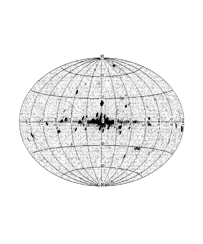
In Figure 1 the raw HEAO1-A2 data is presented in a Hammer-Aitoff, Galactic projection. The data consists of one complete scan of the sky using the Total band ( Allen et al (1994)).

The darkest pixels are associated with individual bright sources and diffuse Galactic emission. Only $\sim 100$ of the brightest sources at high galactic latitudes can be identified ( Piccinotti et al (1982)) identifies 17 galactic and 68 extragalactic sources). In all of the following we restrict ourselves to $|b|>20^{\circ}$ where complete catalogs are available.

The data is first corrected for the locally estimated instrumental background. This is achieved by using both the LFOV and SFOV data to solve the following two equations at each pixel for $I_{background}$: $I_{sfov}=I_{background}+I_{sky}$ and $I_{lfov}=I_{background}+2.26I_{sky}$, where the factor of 2.26 is the ratio of area solid-angle products for the LFOV and SFOV. To reduce noise in the background estimate we then correct the data by subtracting the mean background estimated in strips of constant ecliptic longitude. Prior to the background calculation we remove sources and mask Galactic regions as described below.

In the course of examining the data we observed a systematic change in the measured flux as a function of observation date. Since the data was taken in great circles through the ecliptic pole, data separated by $180^{\circ}$ in ecliptic longitude correspond to approximately the same epoch of observation. Taking the mean flux at fixed longitude of the source removed/masked data (see below), wrapped by $180^{\circ}$ we discovered a clear linear trend in the observed counts. In Figure 2 we plot the observed effect in the Total band data. The least squares linear models for all 4 HEAO colours are shown in Figure 3. The slopes of the trends (in units of counts/sec, vs longitudinal pixel index) are $-0.000716,-0.000194,-0.000357,-0.000265$ for the Soft, Hard, Total and R15 colours respectively, with maximum and minimum at longitudinal pixel indices 69 and 429 respectively.

The time dependent term therefore ranges from $0-7\%$ of the mean intensity for the Soft band, and less for the other colours. In all subsequent analysis the HEAO data has been corrected by subtracting the least squares trend. The resulting change on all quantities discussed is small and always less than 10%.

To improve computational efficiency in all the following analysis we have re-binned the data (following background, and systematics correction, and source removal as described below) into $3^{\circ}\times 6^{\circ}$ pixels in ecliptic coordinates (smaller resolution pixels are more strongly correlated due to the instrument beam)

3 Large scale structures in the HEAO data

Unlike many all-sky catalogues (e.g. IRAS, optical surveys etc.) the ability to unambiguously separate foreground (Galactic/local emission) from background (extragalactic) information is limited in the HEAO X-ray data. The total number of resolved foreground and background sources is small ($\sim 100$) and a detailed model of possible large scale Galactic emission is hard to determine. The Galactic $2-60$ keV emission model of Iwan et al (1982) predicts that some 2% of the observed emission at the galactic poles in the A2 band is of Galactic origin. The largest contribution at latitudes $b\geq 20^{\circ}$ is 5%. (The Iwan model predicts galactic contributions of up to 10% at low latitudes, although there is certainly another, more centrally concentrated component as well ( Worrall et al (1982); Warwick et al (1985); Valinia & Marshall (1998)). More recently, studies in the soft bands ($<0.75$ keV) by ROSAT ( Snowden et al (1997)) indicate that, at these lower energies, the picture is more complicated, with structure at all scales. Whether this soft emission distribution is a good indicator of the much harder $>2$ keV emission is unclear; the galactic contribution in this soft band is almost certainly larger than that above 2 keV, and is potentially more variable as well. In this present work we attempt to at least qualitatively evaluate the likely foreground vs. background contributions to further constrain our estimates of the extragalactic flux anisotropy. In order to evaluate the structure in the map of Figure 1 we use spherical harmonic analysis to filter the high (noisy) frequencies from the map and to reconstruct the flux variations (e.g. Scharf et al 1992). Briefly, the map is expanded into the orthonormal set of spherical harmonics ($Y_{lm}(\theta,\phi)$) by determining the harmonic coefficients as a sum over the flux cells:

$$a_{lm}=\sum_{i}I_{i}\Delta\omega_{i}Y_{lm}^{*}({\hat{\omega}_{i}})\;\;\;,$$ (1)

where $I_{i}$ is the mean surface brightness in a cell, $\Delta\omega_{i}$ is the cell area in direction ${\hat{\omega}_{i}}$. The surface brightness at any point can then be reconstructed using only lower order harmonics, where the resolution is determined by the highest harmonic and goes as $\sim\pi/l_{max}$. In our definitions below the monopole $M_{x}$ is defined as $4\pi\bar{I}$ thus $a_{00}\equiv\sqrt{4\pi}{\bar{I}}=M_{x}/\sqrt{4\pi}$.

3.1 Higher order anisotropies

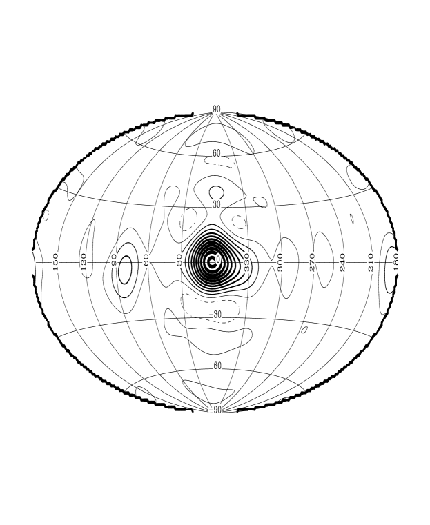
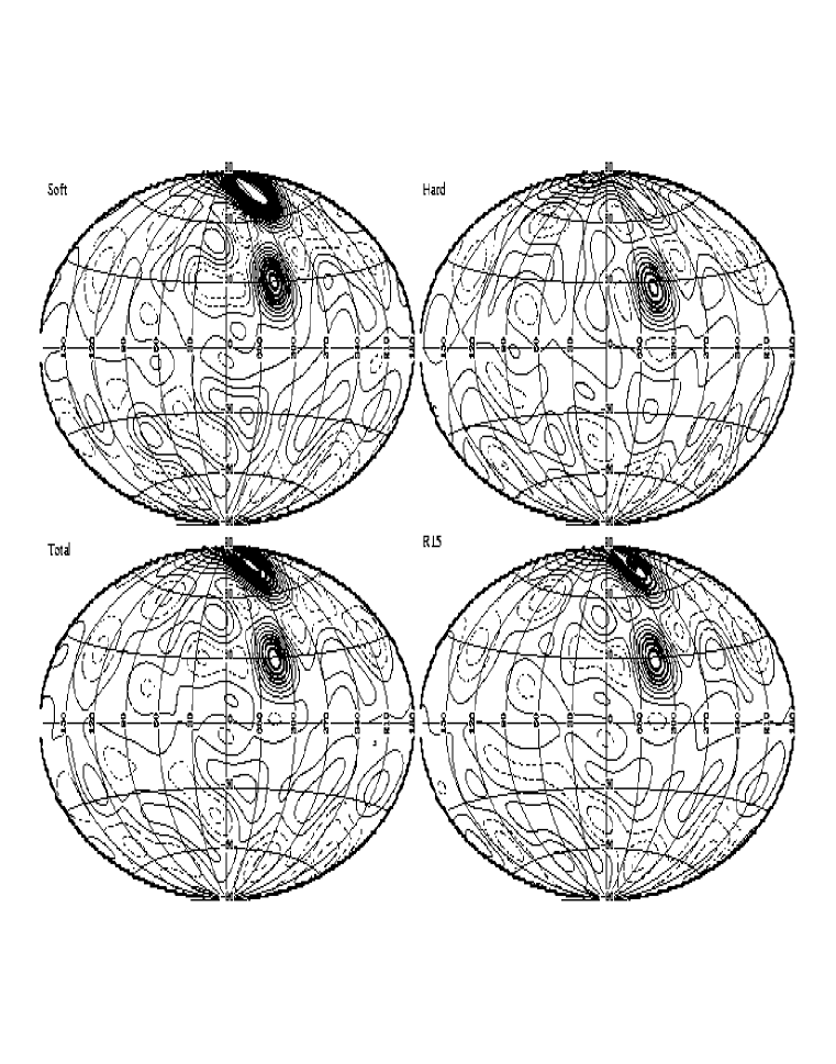
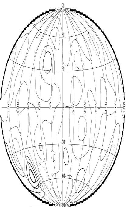
In Figure 4 a harmonic reconstruction of the raw (Total band) HEAO data is shown to a resolution of $\sim 18^{\circ}$ ($l_{max}=10$). The data is clearly dominated by emission associated with the Galaxy (either resolved or unresolved sources). As a first step towards removing this foreground we construct a ‘mask’ using the list of resolved and identified Galactic X-ray sources ( Piccinotti et al (1982)) and a $|b|<22^{\circ}$ Galactic Plane mask. Regions of sizes varying from $\sim 8^{\circ}$ diameter to $12^{\circ}$ diameter are excised around resolved sources, larger regions are removed around the Large and Small Magellanic Clouds (LMC, SMC). A total of $\sim 38$% of the sky area is removed by this mask. The results are dramatic, in Figure 5 the harmonic reconstruction (to $l_{max}=10$) of the data is shown in all four bands, with the above Galactic masking applied. Those regions excised have been filled with the new mean flux as a first order correction (see discussion of dipole estimation below). As described in Section 2, the count/sec in each colour are weighted to be equivalent for emission with a photon index of -1.7. The observed differences in the structure between (for example) the Soft and Hard bands can then be directly interpreted as spatial differences in the mean spectral index of X-ray emission (modulo variations in the signal-to-noise).

Two strong flux enhancements are apparent. The uppermost (at $b\lower 2.15277pt\hbox{$\;\buildrel>\over{\sim}\;$}80^{\circ}$ and spanning the Northern Galactic cap) we associate with the Virgo and Coma clusters. The lower peak (at $l\sim 315^{\circ}$ and $b\sim 30^{\circ}$) is close to the Centaurus/Great Attractor region (e.g. Scharf et al 1992, Webster et al 1998). However, we note that it is also closer to the Galactic Plane and may not be free of Galactic contamination.

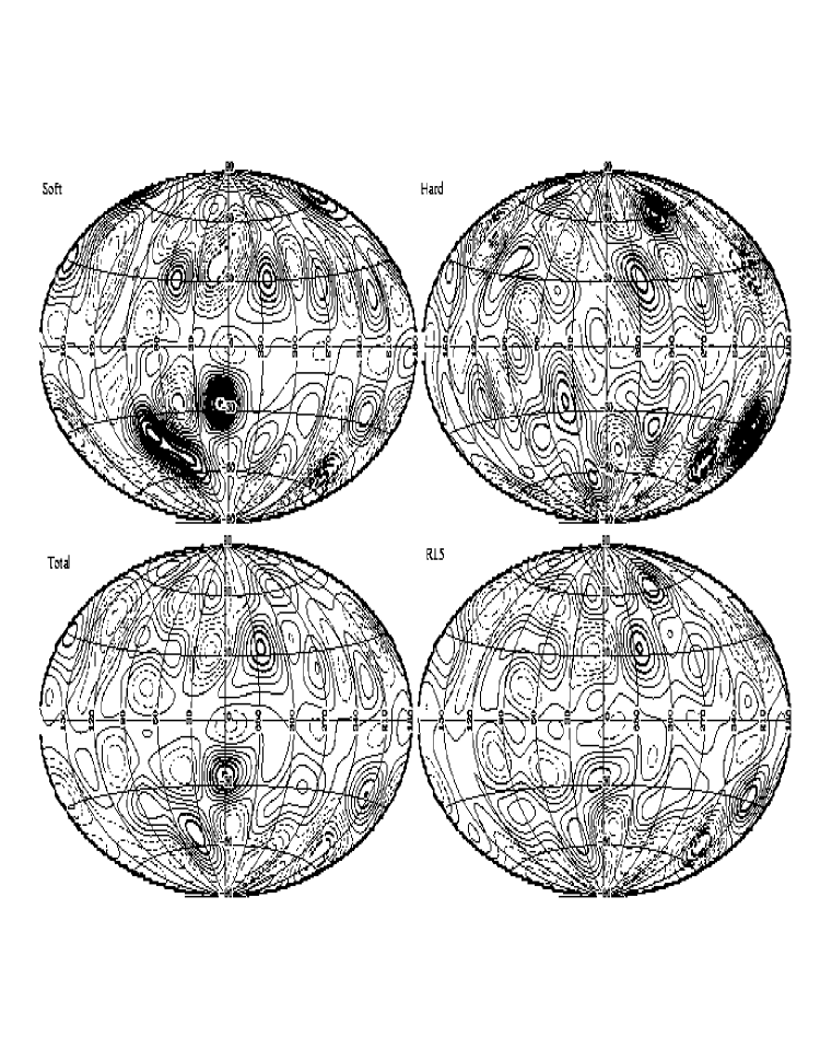
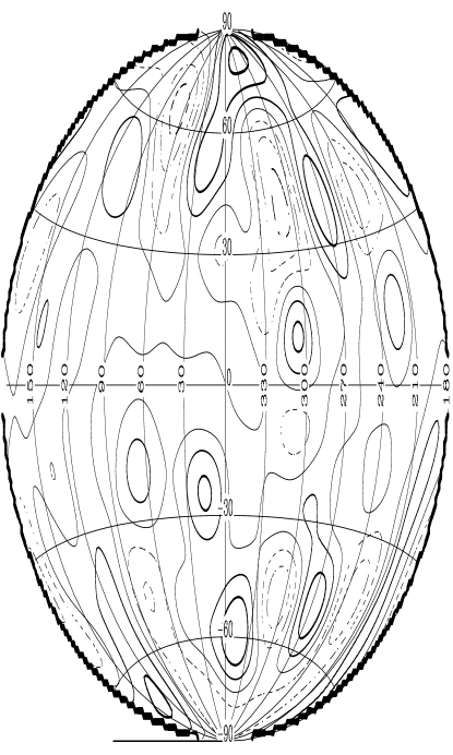
Next we make use of the Pincinotti (1982) catalogue of extragalactic sources (supplemented with the clusters of Edge et al (1990) with $z<0.003$) and excise these regions (in $\sim 8^{\circ}$ diameter cuts) in addition to the above Galactic masking. This results in a dataset with all sources removed down to a flux limit of $3\times 10^{-11}$ ergs s^-1 cm^-2 (c.f. Treyer et al 1998). The median redshift of sources in the extragalactic Piccinotti sample is known to be $z\sim 0.02$. In a further effort to remove all significant X-ray sources from within the local volume, we have made use of the HEAO A1 catalogue of source detections (Ron Remillard, private communication). Using this data we have removed all sources to a slightly lower flux limit of $2\times 10^{-11}$ ergs s^-1 cm^-2 (2-10 keV). We determine this flux limit value from both our chosen limiting count rate in the A1 catalogue (0.006 ct/s) and by normalising with respect to the extrapolated Piccinotti LogN-LogS. This yields a final monopole value corresponding to $M_{x}\simeq 6.2\times 10^{42}$ erg s ^-1 Mpc^-2. The final unmasked sky area is 48%, in Figure 6 the corresponding harmonic reconstructions (to $l_{max}=10$) are shown.

From the X-ray luminosity functions of Grossan (1992) and Boyle et al. (1998), we estimate that the mean luminosity of the local X-ray source population is $L_{\star}\sim 5\times 10^{42}$ erg s^-1, assuming a lower luminosity cutoff of $10^{42}$ erg s^-1 and a present day Hubble constant H₀=100 kms^-1Mpc^-1. As the luminosity function is dominated by faint objects and and the low-luminosity cutoff is somewhat arbitrary, $L_{\star}$ is likely to be a lower limit. Removing sources brighter than $2\times 10^{-11}$ erg s^-1 cm^-2 corresponds to removing all sources brighter than $L_{\star}$ out to $z\sim 0.015$, and all sources brighter than $10\times L_{\star}$ out to $z\sim 0.05$. Therefore most X-ray sources with $z>0.015$ are still unresolved and contribute to the measured dipole (see below).

The contour levels in Figure 6 are approximately a factor $\sim 3$ more exaggerated relative to the mean than in Figure 5. Unlike the extragalactic sky dominated by resolved sources, significant differences in structure is now seen between the Soft and Hard colours. Notably, in the Soft band two strong patches are seen at $(\sim 10^{\circ},\sim-28^{\circ})$ and $(\sim 80^{\circ},\sim-40^{\circ})$, and a significant structure at $l\simeq 180^{\circ}$, extending over $15^{\circ}\lower 2.15277pt\hbox{$\;\buildrel<\over{\sim}\;$}b\lower 2.15277pt\hbox{$\;\buildrel<\over{\sim}\;$}80^{\circ}$. In the Hard band the most significant features are seen at $(\sim 200^{\circ},\sim-40^{\circ})$ and $(\sim 280^{\circ},\sim 60^{\circ})$. Possible identifications with known structures are given in the Figure 6 caption.

In Figure 7 we plot the harmonic reconstructions of ‘noise’ skies for both the Galactic and full extragalactic mask cases in Figures 5 & 6, to provide a qualitative guide to the significance of features. From these figures we can assess the signal-to-noise of structures seen in Figures 5 & 6 (Total band). The most significant individual features are typically a factor 2-3 higher in counts/sec when compared to the equivalent peaks in the pure noise levels. It is apparent that there are at least two likely real, positive, features in Figure 5 and possibly four in Figure 6.

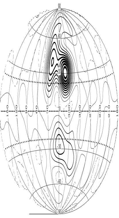
In an attempt to assess the likely amplitude and morphology of Galactic contamination in the HEAO1-A2 data we have analysed the all-sky X-ray data from the ROSAT All Sky Survey (RASS) using the maps of Snowden et al (1997, 1995). In Figure 8 we present a harmonic reconstruction of the 1.5 keV RASS data, subject to the same Galactic and extragalactic source mask as the HEAO1-A2 data as shown in Figure 6. The RASS data was used in a $480\times 240$ pixel Hammer-Aitoff Galactic projection as available from the online archives, no further processing was made, other than filling empty pixels with the mean flux after applying the HEAO1-A2 Galactic and extragalactic source masks. As discussed in Snowden et al (1995) the 1.5 keV band data spans the energy range $\sim 0.7-2$ keV, with essentially no counts above 2 keV. The HEAO1-A2 Hard band is therefore the only colour with no response in this energy range. The response in the other bands is also modest at 2 keV, the effective area is down from its maximum by factors of $\sim 3$, 10, and 10 for the Soft, Total, and R15 colours. The three most prominent features in the RASS reconstruction are concident with the features identified in Snowden et al (1995) as the Northern Spur/Loop I ($l\sim 20^{\circ},b\sim 40^{\circ}$), and the northern and southern parts of a Galactic Bulge emission ($l\sim 340^{\circ},b\sim 30^{\circ}$, $l\sim 0^{\circ},b\sim-30^{\circ}$).

The location of the two Bulge structures is particularly worrying for our interpretation of the structures in Figure 6. In particular the southern structure seen most strongly in the Soft band at $l\sim 10^{\circ},b\sim-30^{\circ}$ is not present in the Hard band data and might indeed be correlated with the RASS southern Bulge feature. Snowden et al (1997) have further investigated the RASS maps and propose that a soft Galactic bulge component is well modelled by a cylindrical volume (with exponential density fall-off away from the Galactic plane) of $\sim 10^{6.6}K$ gas. As discussed above, this does not preclude Galactic bulge emission above 2 keV, but for a thermal spectrum very little emission would be expected. The southern HEAO ’Bulge’ feature appears to fall into this category. The HEAO structure at $l\sim 325^{\circ},b\sim 30^{\circ}$ is however present in all 4 colours, which suggests that while it could be contaminated by the northern Bulge feature, it is more likely to have an extragalactic origin. Therefore, we conservatively estimate that at least 1 out of 3 of the dominant faint (soft), unresolved structures in the HEAO1-A2 data may be Galactic in origin. This is consistent with the detailed investigation of the RASS 1.5 keV dipole made by Plionis & Georgantopoulos (1999) who estimated that $20-30$% of the total background is Galactic in origin in that data.

Without much more rigorous cross-comparison any correlations of the RASS with HEAO1-A2 should be made with caution, since the intrinsic spatial resolution of the RASS ($\sim 2^{\circ}$) is significantly different to that of the HEAO1-A2. In Section 5 below we investigate the effect on the flux dipole of Galactic emission as described by the Iwan et al (1982) model, as well as the effect of removing the putative ‘Southern Bulge’ feature.

4 Angular power spectra

In an associated paper (Treyer et al (1998)) we have investigated the angular fluctuations of the XRB in the context of models of large scale structure (as formulated by LPT97).

Following the formalism used in those papers the total predicted angular power (taken as an ensemble average) is a combination of a large-scale structure component (signal) and a component due to the discreteness of sources (shot-noise):

$$\left<|a_{l}^{m}|^{2}\right>_{model}=\left<|a_{l}^{m}|^{2}\right>_{LSS}+\left<|a_{l}^{m}|^{2}\right>_{SN}$$ (2)

This is then convolved with the foreground mask to produce the observed angular power spectrum:

$$\left<|c_{l}^{m}|^{2}\right>=\sum_{l^{\prime}m^{\prime}}|W_{ll^{\prime}}^{mm^{\prime}}|^{2}\left<|a_{l^{\prime}}^{m^{\prime}}|^{2}\right>$$ (3)

Finally we normalize over the monopole, and for total signal use the notation:

$$C_{l}=\frac{(\left<|c_{l}^{m}|^{2}\right>_{LSS}+\left<|c_{l}^{m}|^{2}\right>_{SN})^{1/2}}{\left<|a_{00}|^{2}\right>^{1/2}}\;\;\;,$$ (4)

(see Section 3).

Figure 9 plots the normalized angular power spectra (i.e. relative to the monopole, Treyer et al (1998), Eqn 14) of the HEAO data for the complete extragalactic plus Galactic mask in all 4 colours. The expected CG effect (see §5 below) has also been subtracted from the data. (Note that in Treyer et al (1998) fewer sources were removed, corresponding to a slightly higher flux limit of $3\times 10^{-11}$ erg s^-1 cm^-2 (2-10 keV)). The Total band spectra used in Treyer et al (1998) are consistent with those shown here, despite some differences in data processing and source removal. The solid curve in Figure 9 is the predicted Total band angular spectra for a low density CDM model with pure X-ray source density evolution and constant, linear biasing (see §6 below and Treyer et al (1998)), and including the predicted noise due to unresolved sources (LPT97).

It is reassuring that the 4 spectra are in generally close agreement (despite different noise characteristics). We do however note that in Figure 9, the Soft band spectra (possibly subject to the most Galactic contamination) shows a strongly discrepant quadrupole ($l=4$) term.

In Figure 10 we also plot the mean spectra obtained from ‘noise’ simulations. As described in Section 5 below these consist of sky fluxes randomly drawn from the real data and masked as per the real data. The complete sky mask is applied both to the data from which fluxes are drawn and to the simulations. The noise estimated from simulations is in agreement with the analytic estimate given in LPT97 and Treyer et al. (1998).

It is apparent that the harmonic shot noise level varies between the HEAO colours. As expected the Total band has the lowest noise level, followed by the R15 band and the highest noise in the Soft and Hard bands, at very similar levels. Comparing these spectra with those in Figure 9 we can see that by $l\sim 5$ in the real data we are approaching the shot noise level and by $l\sim 10$ we have practically reached the shot noise level.

5 The observed flux dipole

The dipole flux anisotropy is described by the harmonic coefficients $a_{1m}$, and can also be written or derived as a simple vector ${\bf D}_{x}$, where;

$${\bf D}_{x}=\sum_{i}I_{i}\Delta\omega_{i}\hat{\bf r}_{i}$$ (5)

We can of course parameterize this differently. For example, the CG effect due to our motion with respect to a radiation field (c.f. CMB dipole etc) is a purely dipolar effect of the form $I^{\prime}=I(1+\Delta\cos\theta)$ where $I$ is surface brightness, and $\theta$ is measured from the direction of motion, in which case $|{\bf D}_{x}|/M_{x}=\Delta/3$ (note that $M_{x}=4\pi\bar{I}$). The factor $\Delta$ for the 2-10 keV X-ray band CG effect is:

$$\Delta=\frac{3v}{c}[1+(\alpha/3)]\;,$$ (6)

where the energy spectral index is $\alpha=0.4$ ( Boldt (1987)). Assuming the Solar velocity with respect to the CMB (Lineweaver et al (1996)), we determine $\Delta=4.2\times 10^{-3}$ for the X-ray CG effect. Here we choose to present the dipole amplitude as $\Delta$ using the above conversion from ${\bf D}_{x}$.

If an all-sky, foreground removed, X-ray surface brightness map existed the flux dipole could be immediately obtained as a vector sum over the flux cells. However, as demonstrated above, removing the foreground involves removing information about the background too. The first order correction to the removal (masking) of regions when the harmonic decomposition is performed is to fill those regions uniformly with the mean density/flux of the unmasked regions. This will not, however, remove cross-talk between the true (full sky, orthonormal) harmonic coefficients (including the dipole) (e.g. Scharf et al (1992)). One solution is to attempt to reconstruct the full sky harmonics by inversion of the coefficient matrix, suitably controlled by (for example) a Wiener filter (e.g. Lahav et al (1994)). While this is a very powerful method it does require a model of the expected harmonic power and a full knowledge of the noise matrix. Additionally, such reconstruction is severely limited by the amount of masking (for a realistic harmonic spectrum of large scale structure), in the case of the HEAO data this is large; if all resolved Galactic and extragalactic sources and the Galactic plane are masked $\sim 52$% of the sky is removed.

In this present work we use two different methods of dipole estimation. First, we perform the vector sum over all flux cells, with a first order correction of filling masked cells with the mean flux over the unmasked regions (the spherical harmonic approach, hereafter Method 1). Second, we perform a least squares fit of a $cos(\theta)$ dependence dipole to the data and determine the best fit $(l,b)$ and $\Delta$ (hereafter Method 2). This latter method does not make use of the masked region, and does not suffer from cross-talk, but it does assume the specific form of the dipole anisotropy, and (unrealistically) that the residuals are negligible. In the following we apply it only to the Total band data, since this data has the best signal-to-noise, and evaluate both methods using Monte-Carlo simulations below.

The results of the various dipole estimations for the HEAO data are presented in Tables 1 and 2 for Methods 1 and 2 respectively.

As a comparison with previous works on the dipole moment of X-ray AGN ( Miyaji & Boldt (1990); Miyaji et al (1991); Miyaji (1994)) we subtract the Total band, source removed extragalactic dipole (row 7, Table 1) from the full extragalactic Total band dipole (row 3, Table 1). The resulting vector (which is equivalent to the dipole vector of the removed extragalactic sources) has $\Delta\simeq 8.2\times 10^{-3}$ and points at $(316^{\circ},53^{\circ})$. Miyaji (1994) found that the flux dipole of resolved AGN (which has different shot noise) in the HEAO1 survey to $z\lower 2.15277pt\hbox{$\;\buildrel<\over{\sim}\;$}0.015$ has a direction $(293^{\circ},33^{\circ})\pm 20^{\circ}$, consistent with this difference vector. In their analysis of the RASS 1.5 keV XRB dipole Plionis & Georgantopoulos (1999) determine a best dipole direction of $(288^{\circ},25^{\circ}$) and amplitude $\Delta=0.051$ (converting their $D_{x}/M_{x}$). While the direction is in general agreement with our results their amplitude is more than a factor of $\sim 10$ higher compared to our results in Tables 1 & 2. This discrepancy is likely due to the increased difficulty of diffuse foreground removal in the soft ROSAT band ($<2$ keV) and an increased soft-band contribution from galaxy clusters and groups. Indeed, Plionis & Georgantopoulos (1999) estimate that Virgo contributes as much as 20% to the RASS dipole amplitude.

As a demonstration of the effect of applying a correction assuming the Iwan et al (1982) Galactic emission model the 3rd block of Table 1 presents the results of removing a Iwan Galactic emission model (normalized to 3% of the monopole) from the distant flux dataset. The effect is relatively modest and systematically decreases the dipole amplitude $\Delta$, and moves the observed dipole direction away from the Galactic center. We also assess the effect of removing the expected CG effect from the data (block 4, Table 1). The dipole is significantly altered; $\Delta$ drops by $15-20$% and the direction changes by as much as $\sim 50^{\circ}$, towards the Galactic center. Combined with a 3% Iwan et al. correction (block 5 Table 1) $\Delta$ is further reduced. We also measure the variation in $\Delta$ (and direction, see Figure 13) as a function of increasing Galactic correction (Figure 11), for cases with and without removal of the expected CG effect (lower and upper curves respectively). In the case in which the CG effect is removed (after the Galactic correction) the amplitude of the Galactic normalization is the most pronounced, reducing $\Delta$ by a factor of 4 between a 1% and 13% correction.

In Table 2 the equivalent results from the Method 2 dipole measurements (using the Total band) are presented. While the directions agree fairly well with those of the Method 1 dipole estimates, the amplitudes appear to be systematically larger by factors $\sim 2.5-3$ (see below).

Finally, we test the effect of removing a $30^{\circ}\times 30^{\circ}$ patch of sky around the putative ‘Southern Galactic Bulge’ region, centred on $l=0^{\circ},b=-25^{\circ}$. As done above this region is filled with the mean flux. The effect on both Method 1 and 2 dipole estimates is small, reducing $\Delta$ by $3-5$% and altering the direction by $\delta\theta\sim 10^{\circ}$.

In order to test the significance of the dipole measurements and the ability of the two methods in recovering a genuine dipole signal we use simple Monte-Carlo simulations. Taking the fluxes of a dataset with the Galactic and extragalactic mask applied we resample the flux distribution and construct a random sky map (equivalent to assuming no correlation between flux cells) which is subject to the same sky incompleteness (in this case the complete mask). The results of harmonic analyses on the simulations over all bands and to $l=20$ have been shown previously in Figure 10. Here we concentrate on the dipolar measurements.

The mean dipole amplitudes over 10 realizations, are shown in Table 3. It is clear that the ‘noise sky’ dipoles are significantly smaller than the dipoles seen in the real data, indicating the presence of genuine correlated structure. The bottom two rows of Table 3 show the result of adding a realistic CG effect to the simulated data. It is encouraging that the estimated amplitudes are close to the input value ($\Delta=4.2\times 10^{-3}$), and the dipole directions are in general agreement, but we note that the two methods appear to differ in a systematic way, with the Method 1 estimate being consistently smaller by a factor $1.5-1.8$. This is not unexpected. As discussed in Treyer et al (1998) and Scharf et al (1992) (and references therein) an incomplete sky creates cross-talk between the harmonic coefficients. In the case of the mask used here the net result is to systematically lower the observed amplitude of the Method 1 dipole. The Method 2 dipole estimate does not suffer from such an effect, although it is a less general estimate of dipole anisotropy. The difference seen in the simulations accounts for at least 50% of the Method 1/2 $\Delta$ discrepancy seen in the HEAO1-A2 data. More detailed simulations would be needed (including realistic fluctuations instead of pure noise) to determine the precise difference expected. A full treatment of the significance of the observed dipole is beyond the scope of this present work.

However, on the basis of the simulations (Table 3) and the results of Tables 1 and 2, we estimate that our observed dipoles are significant at greater than a $\sim 2-3\sigma$ level, and have a typical direction error of $\sim 30^{\circ}$.

6 The flux dipole and bulk motions

The X-ray flux dipole observed at frequency $\nu_{0}$ is defined as:

$${\bf D}_{x}\equiv\sum_{i}f_{i}(\nu_{0})\hat{{\bf r}_{i}}\;,$$ (7)

where the sum is over all directions in the sky, and $f_{i}(\nu_{0})$ is the integrated X-ray flux in the direction $\hat{{\bf r}_{i}}$.

Following the formalism given in LPT97 and assuming linear, epoch-dependent biasing $b_{x}(z)$, such that fluctuations in X-ray sources and mass are related by $\delta_{x}(r_{c},\hat{\bf r})=b_{x}\delta(r_{c},\hat{\bf r})$, then:

$${\bf D}_{x}=\int\int\phi(L_{\nu},z)\frac{L_{\nu}(1+z)}{4\pi r_{L}^{2}}[1+b_{x}(z)\delta(r_{c},\hat{\bf r})]\hat{\bf r}\ dV_{c}dL_{\nu}\;,$$ (8)

where $\phi$ is the radial probability of a source with luminosity $L_{\nu}$ at redshift $z$ and $\delta$ is the mass density contrast.

If the number density of the X-ray sources evolves as $(1+z)^{d}$, their luminosity as $(1+z)^{e}$, and $L_{\nu}\propto\nu^{-\alpha}$, then we can define $q=d+e-\alpha+1$ and the X-ray volume emissivity as:

$$\rho_{x}(z)\equiv\int L_{\nu}\phi(L_{\nu},z)(1+z)\;dL_{\nu}=\rho_{x}(0)(1+z)^{q}~{}.$$ (9)

The dipole can then be written in the form of a “dipolar Olbers’ integral”:

$${\bf D}_{x}=\frac{1}{4\pi}\int\frac{\rho_{x}(z)b_{x}(z)\delta(r_{c},\hat{\bf r})}{r_{c}^{2}(1+z)^{2}}\hat{\bf r}\;dV_{c}\;$$ (10)

Recall that in an Einstein-de Sitter Universe ($\Omega_{0}=1$) $dV_{c}=r_{c}^{2}dr_{c}d\omega$ and $r_{c}=2r_{H}[1-(1+z)^{-1/2}]$, where $r_{H}=c/H_{0}$ is the Hubble radius.

As we do not have a model for $\delta({\bf r})$ in our neighbourhood, we can only make statistical predictions using a model for the power-spectrum $P(k)$ (LPT97, Treyer et al 1998). Of course, what we observe is a single realization and this one realization may not be well represented by the rms value. The rms dipole ($l=1$) can be expressed as (see Eq. 7 in Treyer et al 1998):

$$\langle|a_{1m}|^{2}\rangle_{LSS}={(r_{H}~{}\rho_{x}(0))^{2}\over(2\pi)^{3}}\int k^{2}{\bar{P}}(k)|\Psi_{1}(k)|^{2}{\rm d}k,$$ (11)

where the window function $\Psi_{1}$ contains the various model parameters:

$$\Psi_{1}(k)=\int_{z_{min}}^{z_{max}}\sigma_{8}b_{x}(z)(1+z)^{q-9/2}j_{1}(kr_{c})W_{cut}(z){\rm d}z~{},$$ (12)

and the function $W_{cut}(z)$ accounts for the removal of sources brighter than a given flux cutoff $S_{cut}$. $\sigma_{8}$ is the usual rms mass fluctuation in an $8$h^-1Mpc radius sphere. As in Figure 8, we use a fiducial model assuming low density CDM, pure density evolution with $q=4.6$ and $z_{max}=1.3$ (based on Hasinger 1998), and constant biasing.

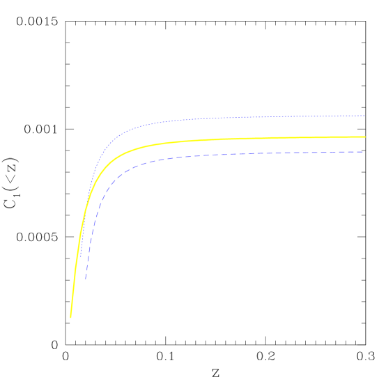
Figure 12 shows the growth of the rms flux dipole as a function of the outer radius cutoff $z_{max}$ for our fiducial cosmological model and 3 scenarios for $W_{cut}(z)$. The figure shows, first, that a flux cutoff of $2\times 10^{-11}$ erg s^-1cm^-2, as used in the present data analysis, is very similar to removing all sources within $z<0.01-0.015$; and secondly, that the rms dipole converges very rapidly, so that most of it originates from $z<0.05-0.1$. Consequently there is very little signal due to structure lying further out, and in the presence of noise we will have effectively no information from $z>0.1$, at least in the rms sense. As the growth of the dipole depends on the power spectrum, $P(k)$, in models with more large scale power the convergence with $z$ will be slower. Note that this convergence is not due to an “Olbers’ effect”. The total intensity ${\bar{I}}$ of the XRB keeps increasing to much higher redshift than do the fluctuations: ${\bar{I}}\propto\int_{0}^{z_{max}}(1+z)^{q-7/2}{\rm d}z~{}$ while $\Psi_{1}(k)\propto\int_{0}^{z_{max}}(1+z)^{q-9/2}j_{1}(kr_{c}){\rm d}z$ (to first approximation). Unlike the monopole, the high redshift fluctuations (dipole and higher harmonics) are effectively washed out by angular averaging over the sky (governed by the Bessel function dependency).

Therefore, we can only use the XRB flux dipole to constrain large scale structures out to 150-300 h^-1 Mpc. Coupled with our estimate that the bright sources we remove are distributed to a distance of $\sim 60$ h^-1Mpc, we should be able to compare our XRB dipole measurement with direct measurements of bulk flows over a similar volume.

In linear perturbation theory the peculiar motion at any point in space is directly proportional to the gravitational acceleration, we can therefore write (assuming all motion was zero a Hubble time ago ( Peebles (1980)):

$${\bf v}\simeq\frac{2}{3}\Omega_{0}^{-0.4}{\bf g}H_{0}^{-1}\;,$$ (13)

where $\Omega_{0}$ is the density parameter. The gravitational acceleration ${\bf g}$ in Newtonian gravity is:

$${\bf g}=G\rho(0)\int\frac{\delta({\bf r})}{r^{2}}\hat{\bf r}\;dV\;,$$ (14)

($\rho(0)$ is the present-epoch mean mass density). We note that this expression only holds in on small scales, by choosing locally Minkowski coordinates (Peebles 1993, p.268). We can therefore approximate Eqn. 10 above for the flux dipole at low redshift to be:

$${\bf D}_{x}=\frac{1}{4\pi}{\rho_{x}(0)b_{x}(0)}{\bf g}/G$$ (15)

Therefore at low redshift the flux of a source follows an inverse square law and if light traces mass in a spatially invariant and linear way then any anisotropies seen in the X-ray data reflect the local gravitational acceleration (assuming linear theory).

We again note that the CG effect produces a dipole pattern on the sky of the form (see Eqn 6):

$$\frac{\Delta I}{\bar{I}}=(3+\alpha)\frac{V_{obs}}{c}cos(\theta)\;\;\;.$$ (16)

Consequently the observed dipole will always be a coupling of the LSS and CG dipole anisotropies.

The well known direct linear-theory relationship between the peculiar velocity and the absolute flux dipole is therefore (from Eqns 13, 14 & 15):

$${\bf v}=\frac{\Omega_{0}^{0.6}}{b_{x}(0)}\frac{H_{0}}{{\rho_{x}(0)}}{\bf D}_{x}\;$$ (17)

(c.f. Boldt 1987, Lynden-Bell et al 1989, Miyaji 1994). To express the linear velocity in terms of the LSS dipole anisotropy $\Delta$ we recall the Olbers integral for $\bar{I}$ (Treyer et al 1998, Eqn 11):

$$\bar{I}=\frac{\rho_{x}(0)r_{H}Q(q,z_{max})}{4\pi}$$ (18)

where the Hubble radius $r_{H}=c/H_{0}$ and $Q(q,z_{max})=((1+z_{max})^{q-2.5}-1)/(q-2.5)$. Since the monopole $M_{x}=4\pi\bar{I}$ and $D_{x}/M_{x}=\Delta/3$, for the fiducial values of $q$ and $z_{max}$ used here we arrive at:

$$|{\bf v}|=2.2\times 10^{5}\Delta\frac{\Omega^{0.6}_{0}}{b_{x}(0)}\;\;kms^{-1}\;\;.$$ (19)

7 Comparison with observed bulk motions

As discussed above, we estimate that the bright sources we remove from the HEAO data are distributed to a distance $\sim 60$h^-1Mpc, we can therefore compare our XRB dipole measurement with direct measurements of bulk flows over this scale.

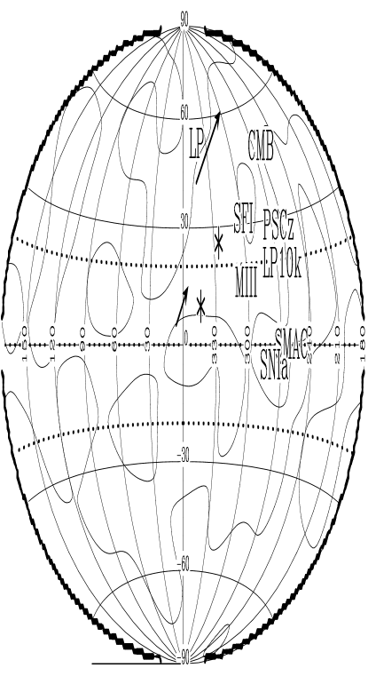
Several studies provide generally consistent estimates of the bulk flow of a $\sim 50$h^-1Mpc radius sphere; $305-370(\pm 110)$ kms^-1 (MIII catalogue, POTENT, Dekel et al 1999), $\sim 300$ kms^-1 (SFI data, Dale et al 1999, Giovanelli et al 1997), $\sim 250$kms^-1 (SNIa data, Riess et al 1995). The directions of these flows are summarised in Figure 13. Using a crude mean of these numbers we estimate $v_{60}\simeq 300\pm 100$ km s^-1. The range of dipoles measured in the Total band (after removal of the dominant X-ray sources from within $\sim 60$ h^-1 Mpc) is $0.0023\leq\Delta\leq 0.0095$ (depending on the measurement method used and corrections for the Galaxy and CG effect). This anisotropy is at most 2 times larger than the expected X-ray CG dipole. Applying Equation 19 the dipole measurements imply that $1/7.1\leq\Omega^{0.6}_{0}/b_{x}(0)\leq 1/1.7$. The favoured Method 2 dipole amplitude given in the last row of Table 2 is $\Delta=0.0065$ which yields $\Omega^{0.6}_{0}/b_{x}(0)=1/4.8$.

The quantity $\Omega_{0}^{0.6}/b_{x}(0)$ has also been estimated from studies of the X-ray selected AGN dipole under certain assumptions about local dynamics. Generally $\Omega_{0}^{0.6}/b_{x}(0)$ ranges from $1/3.5$ if all the local gravitational acceleration is assumed to arise from the volume with $R\lower 2.15277pt\hbox{$\;\buildrel<\over{\sim}\;$}45$ h^-1Mpc, to $1/7$ if only half of the acceleration arises from within this volume (Miyaji (1994)). Using the new IRAS-PSCz survey, Schmoldt et al (1999) predict that some 65% of the LG acceleration is generated within 40h^-1Mpc and that convergence is not reached until $\sim 140$h^-1Mpc. Therefore $\Omega_{0}^{0.6}/b_{x}(0)$ is almost certainly larger than $1/3.5$ using this method. These results are in good agreement with our above constraints from bulk flows and the HEAO dipole. The observed HEAO dipole therefore appears to be quite compatible with current measurements of the bulk flow of the local $\sim 60$h^-1Mpc volume. The dominant population of X-ray emitters (AGN) in the 2-10 keV band is then highly biased with respect to other tracers, e.g. optical or IRAS galaxies.

Over larger scales ($\sim 100-150$h^-1 Mpc) there is less agreement on the reality of bulk flow measurements. For example, the work of Lauer & Postman (1994) has suggested, with much controversy, that the Local Group has a motion relative to the $z<0.05$ Abell cluster frame of 561$\pm 284$ kms^-1 in a direction $l=220^{\circ}$, $b=-28^{\circ}(\pm 27^{\circ})$. Assuming a dynamical origin of the observed CMB dipole this implies that the Abell cluster frame (to $z=0.05$) is itself moving in bulk with respect to the CMB frame with velociy of 689$\pm 178$ kms^-1 towards $l=343^{\circ}$, $b=52^{\circ}(\pm 23^{\circ})$. If correct this could imply that $\sim 50$% of the Local Group motion is due to matter on scales $>100$h^-1Mpc. This specific result has been strongly refuted by several other works (e.g. Riess et al 1995, Giovanelli et al 1997, Hudson et al 1999, Muller et al 1998, Dale et al 1999). More recently however, independent observational evidence for bulk motion over these scales has emerged, in the range of $\sim 600-700$ km s^-1 (e.g. Hudson et al 1999, Willick 1998). All such studies however obtain directions for these motions greater than $60^{\circ}$ away from the LP result, and are themselves highly fraught with potential systematic effects.

In criticism of these results it can be noted that there is an inconsistency between (for example) the Lauer & Postman measurement and the results of gravity dipole estimation using galaxy catalogues. For example, the results of Strauss et al (1992) using the 1.2Jy IRAS redshift survey found an extraordinary convergence of the direction of the inferred gravity dipole out to $\sim 20,000$kms^-1. This convergent dipole direction is only some 20^∘ from the CMB dipole direction. (There are good arguments why the velocity dipole of the Local Group is not necessarily converged until $z\sim 1$ ( Peacock (1992)), but that does not preclude a genuine convergence in a smaller volume). Recently the IRAS-PSCz survey has largely confirmed these observations (Schmoldt et al 1999).

Scaling our above estimates for the HEAO XRB dipole anisotropy we predict that, if all X-ray sources within $\sim 100-150$h^-1Mpc were removed then a 700 km s^-1 bulk flow would correspond to $0.0054\leq\Delta\leq 0.0225$ (assuming the measured range of allowed $\Omega_{0}^{0.6}/b_{x}(0)$). This would be some $1.5-5.0$ times larger than the expected X-ray CG dipole amplitude.

The directions of both the bulk flow estimated from other works, and our present dipole measurements are however scattered over a large area of the sky. Figure 13 summarizes most of these directions. As already mentioned, the LP flow direction is $\lower 2.15277pt\hbox{$\;\buildrel>\over{\sim}\;$}60^{\circ}$ from all others, the Hudson et al (1999) result is also significantly further from the Solar CMB velocity direction. Interestingly the HEAO1-A2 measurements appear to be somewhat intermediate to the LP result and the majority of the other, more local volume, estimates (SFI, MIII, PSCz). However, recalling that we estimate an XRB dipole direction error of at least $\sim 30^{\circ}$ for either method, then the HEAO dipole directions are not inconsistent with (for example) the SFI and MIII flows.

8 Summary and Conclusions

The HEAO1-A2 X-ray data offers the best all-sky survey of baryonic matter to $z\simeq 4$ currently available. Although low level anisotropies in the X-ray sky background arise largely from Galactic contributions, relatively crude foreground removal clearly demonstrates the presence of extragalactic emission associated with well known large scale structure (Virgo, Coma, Centaurus/Great Attractor etc.) in the local universe.

Qualitative comparison of the RASS 1.5 keV data with the 4 HEAO1-A2 bands used here suggests that at least one third of the faint, unresolved HEAO1-A2 structure may be Galactic in origin, and possibly associated with the Galactic Bulge.

The local extragalactic hard X-ray emission is dominated by AGN and galaxy clusters. If we remove the flux associated with these sources to a flux limit of $2\times 10^{-11}$ erg s^-1 cm^-2 (2-10 keV) (which removes all sources more luminous than $5.2\times 10^{42}$ erg s^-1 (2-10 keV) out to $z\simeq 0.015$) we measure a dipole anisotropy of $\Delta=0.0023$ to 0.0095 (depending on the method used and the details of the data processing). This range of anisotropy is consistent with our expectations (LPT 97) of comparable amplitude CG and LSS dipoles. It is significantly smaller than that measured in the RASS 1.5 keV all-sky data by Plionis & Georgantopoulos (1999). However, we have argued that the hard ($>2$ keV) band XRB suffers less from Galactic contamination and have shown how removal of the foreground of bright sources reduces the dipole amplitude and shot noise (see also Treyer et al 1998).

We have derived the fully cosmological expressions for X-ray dipole anisotropy. Unlike the often used Euclidean case, the relationship of the local acceleration to the dipole anisotropy is no longer straightforward. However, in the case of the current HEAO dataset we show that for reasonable choice of cosmology and matter density fluctuation power spectrum most of the dipole anisotropy arises from $z\lower 2.15277pt\hbox{$\;\buildrel<\over{\sim}\;$}0.1$ and the low-redshift, linear theory approximation can be used.

Using current estimates of the bulk flow of the local 60h^-1 Mpc radius volume and our XRB dipole measurements we find that $1/7.1\leq\Omega^{0.6}_{0}/b_{x}(0)\leq 1/1.7$. With our preferred dipole anisotropy measurement then $\Omega^{0.6}_{0}/b_{x}(0)=1/4.8$. This implies that the population of X-ray sources is highly biased with respect to optical or infra-red selected objects. Studies of the dipole anisotropy of the local AGN distribution (Miyaji 1994), and other analyses of the HEAO data (Boughn et al 1998, assuming epoch-independent biasing) also yield high values. Interestingly our previous analysis of the angular power spectrum of the HEAO dataset (Treyer et al 1998) which included terms as high as $l=20$ yielded a present-epoch biasing factor $b_{x}(0)\sim 1-2$. The model fit to this data was however not particularly good, and the lower order harmonics ($l=1-3$) are better fit with a higher $b_{x}(0)$. If $\Omega_{0}=0.3$ then the values of $b_{x}(0)$ estimated from the HEAO dipole/bulk flows fall into this lower range, however our formalism is all based on an $\Omega=1$, Einstein-de-Sitter cosmology. We also note that in all conventional models the bulk flow amplitude of a sphere with radius $R$ drops with $R$ (specifically, if $P(k)\propto k^{n}$ then $V_{bulk}\propto R^{-(n+1)/2}$). Therefore, if we overestimate the volume within which we remove X-ray emission, but continue to apply the observed bulk flow amplitudes for a larger sphere, we will then underestimate $\Omega^{0.6}_{0}/b_{x}(0)$ from Equation 15.

If $\sim 700$ km s^-1 bulk flows over $100-150$ h^-1 Mpc radius volumes did exist, as suggested by some studies (e.g. Lauer & Postman 1994 , Willick 1998, Hudson et al 1999), then we predict that an XRB dipole anisotropy of $0.0054\leq\Delta\leq 0.0225$ would be seen after removing source emission within this volume.

It is worth noting that we should not discount further complications such as a spatially varying local X-ray emmissivity to mass biasing. Indeed, in their study of the X-ray properties of the Great Attractor region and the Shapley supercluster Raychaudhury et al (1991) found that for these similarly massive regions the number counts of X-ray luminous clusters is quite different (Shapley having the most). This is suggestive of a spatial variation in cluster formation and brings into doubt the naive linear biasing scheme.

To fully exploit this, or future, hard X-ray all-sky data for cosmological or dipole studies a better knowledge of the foreground contamination is essential. In particular, a significantly more detailed model of the Galactic (and local, e.g. LMC, SMC) emission is needed. Probably the best way to achieve this will be through the use of softer band data (to provide spatial parameters) combined with point-by-point spectroscopic information which will allow extrapolation to the harder, less contaminated X-ray bands. A spectroscopy capable all-sky imaging survey, such as that discussed by Jahoda (1998) would be well suited to this (see also discussion in Treyer et al (1998)).

Dataset	HEAO band	Amplitude ($\Delta$)	Direction
Galactic Mask	Soft	0.0132	($325^{\circ},51^{\circ}$)
	Hard	0.0084	($355^{\circ},45^{\circ}$)
	Total	0.0114	($327^{\circ},51^{\circ}$)
	R15	0.0111	($324^{\circ},53^{\circ}$)
Complete Mask	Soft	0.0036	($343^{\circ},35^{\circ}$)
	Hard	0.0060	($29^{\circ},2^{\circ}$)
	Total	0.0036	($345^{\circ},43^{\circ}$)
	R15	0.0030	($346^{\circ},48^{\circ}$)
Complete Mask	Soft	0.0033	($336^{\circ},40^{\circ}$)
3% Iwan model	Hard	0.0032	($32^{\circ},2^{\circ}$)
removed	Total	0.0034	($338^{\circ},47^{\circ}$)
	R15	0.0029	($337^{\circ},54^{\circ}$)
Complete Mask	Soft	0.0030	($3^{\circ},-3^{\circ}$)
CG effect	Hard	0.0048	($41^{\circ},-27^{\circ}$)
removed	Total	0.0027	($8^{\circ},5^{\circ}$)
	R15	0.0022	($15^{\circ},0^{\circ}$)
Complete Mask	Soft	0.0025	($1^{\circ},-4^{\circ}$)
CG effect &	Hard	0.0045	($18^{\circ},-44^{\circ}$)
3% Iwan	Total	0.0023	($6^{\circ},6^{\circ}$)
removed	R15	0.0017	($15^{\circ},1^{\circ}$)

Table 1: Spherical harmonic (Method 1) dipole measurements of HEAO1-A2 data, directions in Galactic coordinates.

Dataset	Amplitude ($\Delta$)	Direction
Galactic Mask	$0.0225\pm 0.0005$	($335^{\circ}\pm 24,46^{\circ}\pm 12$)
Complete Mask	$0.0095\pm 0.0005$	($344^{\circ}\pm 24,35^{\circ}\pm 12$)
Complete Mask	$0.0090\pm 0.0005$	($327^{\circ}\pm 24,25^{\circ}\pm 12$)
3% Iwan model removed
Complete Mask	$0.0085\pm 0.0005$	($353^{\circ}\pm 24,1^{\circ}\pm 12$)
CG effect removed
Complete Mask	$0.0065\pm 0.0005$	$(342^{\circ}\pm 24,7^{\circ}\pm 12$)
CG effect &
3% Iwan removed

Table 2: Least squares fit (Method 2) dipole amplitudes of Total band HEAO data. Errors correspond to finite search grid scales.

Simulation	Dipole measure	Mean Amplitude ($\Delta$)	Mean sepn. from $(265^{\circ},48^{\circ}$)
Complete Mask,	Method 1	$0.00135\pm 0.00031$	–
randomized fluxes	Method 2	$0.0022\pm 0.0014$	–
+ 4.2$\times 10^{-3}$ CG effect	Method 1	$0.0024\pm 0.0007$	$31^{\circ}\pm 20^{\circ}$
	Method 2	$0.0043\pm 0.0015$	$25^{\circ}\pm 15^{\circ}$

Table 3: Flux dipole measurements from simulations. Amplitudes are taken as the mean over 10 realizations, errors correspond to $1-\sigma$ standard deviations.

Figure 1: The full HEAO1-A2 Total band data shown in Hammer-Aitoff Galactic coordinates projection. The Galactic Plane is clearly visible. Emission from the Large and Small Magellanic Clouds is visible towards the bottom of the plot, close to the southern ecliptic pole.

Figure 2: The mean counts/sec averaged over the time-wrapped Total band data (subject to Galactic masking) as a function of longitudinal pixel index. The least squares linear model is shown as the solid line.

Figure 3: The least squares linear trends to the time-wrapped HEAO data averaged at each longitudinal index using the complete source and Galaxy mask. Solid line - Soft band, dotted line - Hard band, short dashed line - Total band, long-dashed line - R15 band.

Figure 4: Harmonic reconstruction to $l_{max}=10$ (angular resolution $\sim 18^{\circ}$) of the raw total band HEAO1-A2 data in Galactic coordinates. Note the complete domination by the Galaxy, in particular X-ray emission from the region of the Galactic centre. The first solid contour is at the mean intensity, subsequent soild contours are above the mean (dashed below) with separation of $\sim 72$% of the mean. The uppermost solid contour is at $\sim$ 720% of the mean.

Figure 5: Harmonic reconstruction to $l_{max}=10$ in Galactic coordinates (angular resolution $\sim 18^{\circ}$) of the 4 HEAO1-A2 bands with a Galactic Plane cut of $|b|<22^{\circ}$ and all resolved Galactic sources removed as well as the LMC nad SMC regions. Masked regions are filled at the mean intensity of the unmasked regions. The first solid contour is at the mean intensity, subsequent solid contours are above the mean intensity, dashed contours are below the mean. Contour separation is 0.04 counts/s in all bands. Associated structures can be identified: Virgo/Coma (at $b\lower 2.15277pt\hbox{$\;\buildrel>\over{\sim}\;$}80^{\circ}$ and spanning the Northern Galactic cap), Centaurus/Great Attractor (at $l\sim 315^{\circ}$ and $b\sim 30^{\circ}$)

Figure 6: Harmonic reconstruction to $l_{max}=10$ of HEAO data with the complete mask applied. Contours are as for Figure 5 but now separated by 0.013 counts/sec. Some of the features seen may be associated with known structures. For example, the feature at $l\sim 80^{\circ},b\sim-45^{\circ}$ may be associated wth the Pegasus cluster/supercluster which extends to $z\lower 2.15277pt\hbox{$\;\buildrel>\over{\sim}\;$}0.04$, the soft feature at $l\sim 10^{\circ},b\sim-30^{\circ}$ may be Galactic (see text) although the Pavo-Indus-Telescopium structure lies in the same direction. The feature at $l\sim 210^{\circ},b\sim-30^{\circ}$ lies in the direction of Abell 530 and 400, and the feature at $l\sim 280^{\circ},b\sim 60^{\circ}$ matches the direction of the Leo cluster/group.

Figure 7: In panels (a) and (b) the $l_{max}=10$ harmonic reconstructions of example total band ‘noise’ skies are plotted for the two mask cases in Figures 5 & 6, using identical contour levels to these figures. The spherical harmonic coefficients are generated from Monte-Carlo realisations as described in Section 5 below, and reflect a random field drawn from the appropriate angular power spectrum in both cases (Section 4). Sky masking is also applied to these noise realisations.

Figure 8: Harmonic reconstruction to $l_{max}=10$ of the RASS 1.5 keV data. The complete HEAO1-A2 mask (Galactic and extragalactic sources removed) has been applied to the data. Horizontal dotted lines at $b=\pm 20^{\circ}$ delimit the Galactic plane mask. Contours are spaced at $\sim 1.7$% of the monopole, uppermost contour is at $\sim 17$% of the monopole

Figure 9: The normalized spherical harmonic power spectrum of the HEAO1 XRB is plotted to $l=20$ for Soft (dotted), Hard (short-dashed), Total (long-dashed) and R15 (dot-dashed) colours. The Galactic mask and extragalactic mask has been applied, corresponding to source removal to a flux limit of $2\times 10^{-11}$ erg s^-1 cm^-2 (2-10 keV). The solid line shows a fiducial ’best-fit’ model for the Total band, as described in (Treyer et al (1998)): low density CDM $P(k)$ with pure X-ray source density evolution and constant biasing ($b_{x}(0)=1$), including the expected noise (see also §6).

Figure 10: The mean angular power spectrum over 10 realizations for each HEAO colour is plotted for ‘noise’ skys. Error bars correspond to the $1-\sigma$ scatter expected between individual realisations.

Figure 11: The Method 1 flux dipole amplitude in the Total band is plotted as a function of increasing Galactic correction (Iwan model, normalised to % of monopole). The upper curve (solid squares) corresponds to the dipole without removal of the expected CG effect, the lower curve (open squares) has had the expected CG effect removed following the Iwan model Galactic correction.

Figure 12: The growth of the rms flux dipole is plotted as a function of outer radius cut-off $z_{max}$ for a low density CDM $P(k)$ with pure density evolution and constant biasing as described in (Treyer et al (1998)). The solid curve assumes $z_{min}=0$ and a flux cutoff $S_{cut}=2\times 10^{-11}$ erg s^-1 cm^-2, while the thin lines simply assume a radial cutoff of $z_{min}=0.01$ (upper dotted line) and 0.015 (lower dashed line) respectively (for both cases $W_{cut}(z)\equiv 1$.

Figure 13: A summary of key directions and dipole results plotted in equal area Galactic coordinates. Alphanumeric keys correspond to: LP - direction of Lauer & Postman (1994) bulk motion in CMB frame, CMB - direction of motion of the Sun in CMB frame (direction of expected CG effect) (Lineweaver et al (1996)), SFI - bulk flow direction of 50h^-1Mpc volume by Dale et al (1999) using SFI data (Giovanelli et al 1997), PSCz - predicted bulk flow in same volume from IRAS PSCz data (Schmoldt et al 1999), MIII - bulk flow in same volume from Mark III, POTENT catalogue (Dekel et al 1999), SNIa - bulk flow in same volume from Riess et al (1995), LP10k - bulk flow of 150 h^-1Mpc volume Tully-Fisher dataset (Willick 1998), SMAC - bulk flow of 120h^-1Mpc volume (Hudson et al 1999). Arrows correspond to Method 1 HEAO1-A2 dipoles with increasing Iwan Galactic corrections (1-13%), upper (higher latitude) and lower arrows correspond to upper and lower curves in Figure 10 (without and with removal of the expected CG effect, respectively). Upper and lower asterix’s label the corresponding Method 2 dipoles with 3% Iwan model corrections (Table 2).

References

- Allen et al (1994) Allen, J., Jahoda, K., and Whitlock, L. 1994, Legacy, 5, 27 (also http://heasarc.gsfc.nasa.gov/docs/journal/heao1-a2_5.html).
- Almaini et al (1997) Almaini, O., Shanks, T., Griffiths, R. E., Boyle, B. J., Roche, N., Georgantopoulos, I., Stewart, G. C., 1997, MNRAS, 291, 372
- Barcons et al (1995) Barcons, X., Franceschini, A., De Zotti, G., Danese, L., and Miyaji, T., 1995, ApJ, 455, 480
- Boldt (1987) Boldt E., 1987, Physics Reports, 146, No. 4, p 215
- Boughn et al (1998) Boughn, S. P., Crittenden, R. G., Turok, N. G., 1998, New Astronomy, 3, 275
- Cagnoni et al (1998) Cagnoni, I., Della Ceca, R., and Maccacaro, T., 1998, ApJ, 493, 54.
- Comastri et al (1995) Comastri, A., Setti, G., Zamorani, G., Hasinger, G., 1995, A&A, 296, 1
- Dale et al (1999) Dale, D. A. et al 1999, ApJ, 510, L11
- Dekel et al (1999) Dekel, A. et al 1999, ApJ in press, preprint astro-ph/9812197
- Edge et al (1990) Edge, A. C., Stewart G. C., Fabian, A. C., Arnaud, K. A., 1990, MNRAS, 245, 559
- Giovanelli et al (1997) Giovanelli, R. et al 1997, AJ, 113, 53
- Grossan (1992) Grossan, A. G. 1992, Ph. D. thesis, Massachusetts Institute of Technology
- Hasinger et al (1998) Hasinger, G., Giacconi, R., Schmidt, M., Trumper, J., Zamorani G., 1998, A&A, 329, 482
- Hudson et al (1999) Hudson, M. J., Smith, R. J., Lucey, J. R., Schlegel, D. J., Davies, R. L., 1999, ApJ, 512, L79
- Iwan et al (1982) Iwan D., Shafer, R. A., Marshall, F. E., Boldt, E. A., Mushotzky, R. F., Stottlemyer, A., 1982, ApJ, 260, 111
- Jahoda et al (1991) Jahoda, K., Lahav, O., Mushotzky, R. F., and Boldt, E. A. 1991, ApJ378, L37
- Jahoda et al (1992) Jahoda, K., Lahav, O., Mushotzky, R. F., and Boldt, E. A. 1992, ApJ399, L107
- Jahoda (1993) Jahoda, K., 1993, Adv. Space Res., 13(12), 231
- Jahoda (1998) Jahoda, K., 1998, Astron. Nachrichten, 319, 129
- Lahav et al (1993) Lahav, O. et al 1993, Nature, 364, 693
- Lahav et al (1994) Lahav, O., Fisher, K. B., Hoffman, Y., Scharf, C. A., Zaroubi, S., 1994, ApJ, 423, L93
- Lahav et al (1997) Lahav, O., Piran T., Treyer M.A., 1997, MNRAS, 284, 499
- Lauer & Postman (1994) Lauer, T. R., Postman, M., 1994, ApJ, 425, 418
- Leiter & Boldt (1992) Leiter, D., and Boldt, E., 1992, in The Compton Observatory Science workshop (see N92-21874 12-90), p359
- Lineweaver et al (1996) Lineweaver, C. H., et al, 1996, ApJ, 470, 38
- Lynden-Bell et al (1989) Lynden-Bell, D., Lahav, O., Burstein, G., 1989, MNRAS, 241, 325
- Madau et al (1994) Madau, P., Ghisellini, G., Fabian, A. C., 1994, MNRAS, 270, L17
- Miyaji & Boldt (1990) Miyaji, T. and Boldt, E. A. 1990, ApJ, 353, L3
- Miyaji et al (1991) Miyaji, T., Jahoda, K., and Boldt, E. A. 1991, in After the First Three Minutes, AIP Conference Proceedings 222, eds. Holt, S. S., Bennett, C. L., and Trimble, V. (New York:AIP) 431
- Miyaji (1994) Miyaji, T. 1994, Ph. D. thesis, Univ. of Maryland, College Park, MD USA.
- Miyaji et al (1994) Miyaji, T., Lahav, O., Jahoda, K., and Boldt, E. A. 1994, ApJ, 434, 424
- Muller et al (1998) Muller, K. R., Freudling, W., Watkins, R., Wegner G., 1998, ApJ, 507, L105
- Mushotzky et al (2000) Mushotzky, R. F., Cowie, L., Barger, A., Arnaud, K., 2000, Nature, 404, 459
- Peacock (1992) Peacock, J. A., 1992, MNRAS, 258, 581
- Peebles (1980) Peebles, P. J. E., 1980, The Large Scale Structure of the Universe, Princeton Univ. Press, Princeton, NJ
- Peebles (1993) Peebles, P. J. E., 1993, Principals of physical cosmology, Princeton Univ. Press, Princeton, NJ
- Piccinotti et al (1982) Piccinotti, G. et al, 1982, ApJ, 253, 485
- Plionis & Georgantopoulos (1999) Plionis, M., Georgantopoulos, I., 1999, MNRAS, 306, 112.
- Postman & Lauer (1993) Postman, M., Lauer, T. R., 1993, in ”Cosmic Velocity Fields”, proceedings of 9th IAP Astrophys. meeting, Eds. Bouchet, F. R. & Lahiechez-Rey, M., Editions Frontieres, p 69
- Raychaudhury et al (1991) Raychaudhury, S., Fabian, A. C., Edge, A. C., Jones, C., Forman, W., 1991, MNRAS, 248, 101
- Refregier et al (1997) Refregier, A., Helfand, D. J., McMahon, R. G., 1997, ApJ, 477, 58
- Riess et al (1995) Riess, A. G., Press, W. H., Kirshner R. P., 1995, ApJ, 445, L91
- Scharf et al (1992) Scharf, C. A., Hoffman, Y., Lahav, O., Lynden-Bell, D., 1992, MNRAS, 256, 229
- Schmoldt et al (1999) Schmoldt, I. et al 1999, MNRAS, 304, 893
- Shafer (1983) Shafer, R. A. 1983, Ph.D. thesis, U. of MD, NASA TM 85029
- Snowden et al (1997) Snowden, S. et al, 1997, ApJ, 485, 125
- Strauss et al (1992) Strauss, M. A., Yahil, A., Davis, M., Huchra, J. P., Fisher, K. B., 1992, ApJ, 397, 395
- Treyer et al (1998) Treyer, M., Scharf, C. A., Lahav O., Jahoda, K., Boldt, E., Piran, T., 1998, ApJ 509, 531.
- Ueda et al (1999) Ueda, Y. et al, 1999, ApJ, 518, 656
- Valinia & Marshall (1998) Valinia, A. and Marshall, F. E. 1998, ApJ, submitted
- Warwick et al (1985) Warwick, R. S., 1998, Nature, 317, 218
- Webster et al (1998) Webster, M., Lahav, O., Fisher, K., 1998, MNRAS, 287, 425
- Willick (1998) Willick, J. A., 1998, preprint astro-ph/9812470
- Worrall et al (1982) Worral, D. M., Marshall, F. E., Boldt, E. A. and Swank, J. H. 1982, ApJ, 255, 111
- Wu et al (1999) Wu, K., Lahav, O., Rees, M. J., 1999, Nature, 397, 225