Thermal Equilibrium Curves and Turbulent Mixing in Keplerian Accretion Disks

Abstract

We consider vertical heat transport in Keplerian accretion disks, including the effects of radiation, convection, and turbulent mixing driven by the Balbus-Hawley instability, in astronomical systems ranging from dwarf novae (DNe), and soft X-ray transients (SXTs), to active galactic nuclei (AGN). In order to account for the interplay between convective and turbulent energy transport in a shearing environment, we propose a modified, anisotropic form of mixing-length theory, which includes radiative and turbulent damping. We also include turbulent heat transport, which acts everywhere within disks, regardless of whether or not they are stably stratified, and can move entropy in either direction. We have generated a series of vertical structure models and thermal equilibrium curves using the scaling law for the viscosity parameter $\alpha$ suggested by the exponential decay of the X-ray luminosity in SXTs. We have also included equilibrium curves for DNe using an $\alpha$ which is constant down to a small magnetic Reynolds number ($\sim 10^{4}$). Our models indicate that weak convection is usually eliminated by turbulent radial mixing, even when mixing length estimates of convective vertical heat transport are much larger than turbulent heat transport. The substitution of turbulent heat transport for convection is more important on the unstable branches of thermal equilibrium S-curves when $\alpha$ is larger. The low temperature turnover points $\Sigma_{max}$ on the equilibrium S-curves are significantly reduced by turbulent mixing in DNe and SXT disks. However, in AGN disks the standard mixing-length theory for convection is still a useful approximation when we use the scaling law for $\alpha$, since these disks are very thin at the relevant radii. In accordance with previous work, we find that constant $\alpha$ models give almost vertical S-curves in the $\Sigma-T$ plane and consequently imply very slow, possibly oscillating, cooling waves.

1 Introduction

The disk-instability model in a thin accretion disk is the most popular model for dwarf-novae (DNe) outbursts and soft X-ray transients (SXTs) (for recent reviews see Cannizzo (1993) or Osaki (1996)). In this model the initial fast rise of luminosity in an outburst is due to the propagation of a heating front at the local thermal speed, while the exponential decay follows from the subsequent slow propagation of a cooling wave. The alternation of heating and cooling in these systems comes from the characteristic ‘S’ shaped curve in the midplane temperature versus column density equilibrium curve (see Fig.  1 below). At all points along this curve the heating due to the local dissipation of orbital energy is balanced by radiative losses and convective heat transport. The unstable middle branch of the equilibrium curve, where column density falls with increasing midplane temperature, is produced by the hydrogen ionization transition and its effect on radiative opacities. The local heating rate is usually taken to follow some variant of the $\alpha$ prescription (Shakura and Sunyaev (1973)). Vertical heat transport in accretion disks is modeled following the usual treatment for radial heat transport in stars, with radiation and convection defining the thermal energy balance. Unlike main-sequence stars which have stable convective zones and internal veloicty fields, convection in accretion disks varies with time as they evolve along the thermal equilibrium curves. Typically, convection has a very strong influence on the structure of the thermally and viscously unstable middle branch of the thermal equilibrium curve since the optically depth of a partially ionized disk is very large.

Convective mixing is not the only source of turbulent transport in stars and disks. Diffusive mixing induced by shear instabilities in rotating stars has been examined by several researchers (Zahn (1992), Maeder (1995), Maeder and Meynet (1996)) for its effects on the luminosity, and evolution of stars. Similarly, it is appropriate to include shear-induced turbulent mixing in the study of accretion disk structure, especially since the luminosity of accretion disks is ultimately due to the dissipation of orbital energy through some sort of shear instability. Turbulent mixing is an unavoidable part of this process. Furthermore, a particular local instability has been identified (Velikhov 1959, Chandrasekhar 1960, Balbus and Hawley 1991, Hawley and Balbus 1992) which is uniquely suited to playing this role, and consequently gives us a theoretical basis for evaluating the efficiency of turbulent mixing. In accretion disks the Velikhov-Chandrasekhar instability is commonly referred to as the Balbus-Hawley instability. Here we abbreviate this as the BH instability. In contrast to convective transport, which only affects the convectively unstable regions and moves heat down temperature gradients, turbulent transport driven by the BH instability is ubiquitous within magnetized accretion disks, and will always act to reduce entropy gradients. The effect of turbulent diffusion due to some sort of shearing instability, not necessarily the BH instability, has been studied in the context of radial transport in thin (important for transition fronts, e.g. see Menou, Hameury, & Stehle (1999)) and advective (Honma (1996)) disks, and in the context of vertical transport in T Tauri disks (D’Alessio et. al. (1998)).

In a real disk the BH instability should generate turbulence which is only moderately anisotropic (Vishniac and Diamond (1992)), an expectation which is consistent with the available numerical simulations (see Gammie 1997 and references contained therein). Consequently, we expect that the dimensionless form of all the transport coefficients should differ only by factors of order unity. More precisely, we note that the numerical simulations consistently suggest that the angular momentum transport is dominated by magnetic tension, and that the relevant magnetic field moment $<B_{r}B_{\theta}>$ is a few times $\rho<v_{z}^{2}>$. The vertical diffusion coefficient is $<v_{z}^{2}>\tau$, where $\tau$ is the velocity correlation time scale, and $\Omega\tau$ is a factor of a few, where $\Omega$ is the local orbital frequency. We conclude that the vertical diffusion coefficient is comparable to the radial diffusion coefficient. In other words,

$$D_{z}\sim\nu,$$ (1)

where $\nu$ is the usual notation for the turbulent kinematic viscosity. Here we will assume that equation (1) is an exact equality, although in reality we expect that this is only a rough approximation. Consequently, if we assume that the turbulent Prandtl number is unity, the vertical thermal diffusion coefficient $\chi_{T}$ can be written as

$$\chi_{T}\sim\nu={2\over 3}{\alpha P\over\rho\Omega},$$ (2)

where $\Omega$ is the Keplerian angular velocity, and $P$ and $\rho$ are the disk pressure and mass density. The turbulent mixing rate across the disk is

$$k_{z}^{2}\chi_{T}\sim\alpha\Omega,$$ (3)

where we have assumed a vertical wavelength $1/k_{z}$ comparable to the vertical global pressure scale height $\lambda_{P}$. Since this is also the thermal equilibration rate for the disk, this implies that turbulent mixing can have a significant effect on disk structure.

The BH instability follows from the presence of a magnetic field in the disk, which requires some sort of magnetic dynamo. The value of $\alpha$ is a fraction of $(V_{A}/c_{s})^{2}$, the ratio of magnetic pressure to ambient pressure. This ratio is determined by the balance between turbulent dissipation and flux generation via the (uncertain) dynamo process. It has long been known that the observed luminosities and timescales for DNe require a larger hot state viscosity, $\alpha_{hot}$, than in quiescence, $\alpha_{cold}$ (Smak (1984), Livio and Spruit (1991)). This could indicate a dependence of $\alpha$ on temperature, or more probably on the disk geometry. On the other hand, it could simply reflect the fact that cold disks have a large neutral fraction and a high resistivity. The latter consideration has led Gammie and Menou (1998) to propose that disks in quiescence are cold enough to shut down all dynamo activity. Evidence in favor of the former idea comes from the observed exponential decay of soft X-ray luminosity for soft X-ray transients which seems to require a scaling law for $\alpha$ of the form (Cannizzo, Chen, and Livio (1995), Vishniac and Wheeler (1996),Vishniac (1997))

$$\alpha\approx\alpha_{0}\left({{c_{s}}\over r\Omega}\right)^{1.5},$$ (4)

where $\alpha_{0}=50$, ${c_{s}}$ is the isothermal sound speed at the mid-plane, and $r$ is the radial position of the annulus. The value of $\alpha_{0}$ is proportional to the assumed masses of the central black holes used to calibrate this relation. Cannizzo et al. assumed a black hole mass of $10M_{\sun}$. This scaling law has been criticized (see e.g. King & Ritter (1998) and references therein) on the grounds that irradiation should substantially modify the structure and stability of disks around black holes. Certainly a naive calculation of the optical emission from the disks of SXTs during the decline from outburst fails to match the observed behavior (Chen, Shrader, and Livio (1997)). However, a recent study (Dubus et al. (1999)) has shown that it is much more difficult for self-consistent models of irradiation to change the basic disk structure (and by extension the X-ray light curve) than to alter the optical emission from the disk.

Equation (4) is not compatible with the original suggestion by Balbus and Hawley (1991) that the dynamo process should saturate in equipartition between the magnetic field and the gas pressure. This suggestion was motivated by the notion that the dynamo process arises from the random stretching of field lines in a turbulent medium (Batchelor (1950), Kazantsev (1967)). On the other hand, this kind of dynamo is rigorously justifiable only in the limit where magnetic forces are negligible, which is obviously not the case here. Equation (4) may be compatible with the notion that the instability gives rise to an incoherent dynamo effect (Vishniac and Brandenburg (1997)), although this predicts a somewhat steeper dependence on geometry as $(c_{s}/r\Omega)\rightarrow 0$. However, the saturation of the instability as the magnetic field approaches equipartition may explain the discrepancy (Vishniac (1999)), and is, in any case, necessary to explain the low sensitivity to geometry seen in the numerical simulations (whose parameters are generally equivalent to $c_{s}/r$ of order unity). We stress that since the dependence is fundamentally one of geometry rather than Mach number, the current generation of numerical simulations are compatible with either model. Here we will explore the consequences of equation (4) for vertical structure, although we will also discuss the alternative, that $\alpha$ is constant down to a limiting value of the magnetic Reynolds number.

Another major issue in vertical structure calculations is the role of convection. Although convection is unlikely to account for any significant level of radial angular momentum transport ($\propto\langle v_{r}v_{\theta}\rangle$, where $v_{r}$ and $v_{\theta}$ are the fluctuating velocity fields) in Keplerian disks (Balbus and Hawley (1998)), it may still play an important role in vertical energy transport ($\propto\langle v_{z}\delta T\rangle$, where $\delta T$ is the fluctuating temperature field). The use of standard mixing length theory (MLT) is even more uncertain in disks than in stars, and previous structure calculations have included simple nonlinear closure schemes (Canuto and Hartke (1986), Cabot et. al. (1987), Cannizzo (1992)), detailed linear analyses of the convective modes (Ruden, Papaloizou, and Lin (1988)), and a reduced effective mixing length (Cannizzo (1992)). Some of these calculations included the assumption that angular momentum transport is mediated by convective motions, so that the results cannot be extended to ionized disks. There is an additional problem with the use of nonlinear closure schemes since such schemes typically fail to reproduce experimental and numerical results in extremely strong shearing environments, although there has been some progress in the intervening years (cf. Speziale et al. 1991; Speziale and Gatski 1997). A particular problem with such schemes is that they tend to underestimate the degree of anisotropy for low Rossby numbers. In any case, none of the previous work included the effect of diffusive damping and mixing due to turbulent motions acting across the reduced radial length scales. How can we determine the ‘typical mode’ of convection (i.e. in the spirit of MLT) when differential rotation and BH turbulence are simultaneously present? To account for nonlinear effects within the context of linear theory, we start with the linear perturbation theory of convection for Keplerian disks and find the modes most resistant to the dissipative effects of shear and turbulent mixing. We use the properties of these linear modes as a guide to the nonlinear state and the typical velocity and eddy size of convective cells. We defer discussion of the empirical basis for this approach to the last section of this paper.

The purpose of the paper is to calculate the vertical structure and thermal equilibrium S-curves for a variety of astrophysical disks, including the effects of turbulent energy transport throughout the whole thickness of the disk, reasonable modifications of MLT for convection in disks, and the scaling formula for $\alpha$ given in equation (4). Standard MLT and the associated vertical energy transport normally used in Keplerian disk models are reviewed in §2. Section 3 describes the turbulent energy flux driven by the BH instability. This energy flux is particularly important if convection is suppressed. We examine the conditions for the suppression of convection in §4. In §5, we propose a new model for vertical energy transport in disks. We present and discuss our results for DNe, SXTs, and AGNs in §6. Finally, we summarize our results and present our conclusions in §7.

2 Standard MLT with a scaling law for $\alpha$

The basic equations for the vertical structure of a geometrically thin, Keplerian, optically thick disk are derived from mass conservation, radiative and convective energy transport, and thermal and hydrostatic equilibrium. These give four differential equations for the column density $\Sigma$, the total vertical energy flux $F$, the total pressure $P$, and the temperature $T$ as a function of distance from the disk midplane: (Meyer and Meyer-Hofmeister (1982), Cannizzo and Cameron (1988))

$${d\Sigma\over dz} = 2\rho=2{P_{g}\mu\over RT},$$ (5)

$${dF\over dz} = {3\over 2}\alpha\Omega P,$$ (6)

$${dP\over dz} = -\rho g_{z}=-\rho\Omega^{2}z=-{P_{g}\mu\over RT}\Omega^{2}z,$$ (7)

$${dT\over dz} = -{3\kappa\rho\over 4acT^{3}}F_{rad}=-{3\kappa\left({P_{g}\mu\over RT}\right)\over 4acT^{3}}\left({\nabla\over\nabla_{r}}\right)F,$$ (8)

where $z$ is the vertical coordinate perpendicular to the disk plane and is zero at the mid-plane, $\mu$ is the mean molecular weight, $\kappa$ is the Rosseland opacity, $F_{rad}$ is the radiative flux, $\nabla$ and $\nabla_{r}$ are defined as $d\ln T/d\ln P$ associated with the radiative flux $F_{rad}$ and the total flux $F$ respectively (Cox and Giuli (1968)):

$$F_{rad} = {4ac\over 3}{T^{4}\over\kappa\rho\lambda_{p}}\nabla.$$ (9)

$$F = {4ac\over 3}{T^{4}\over\kappa\rho\lambda_{p}}\nabla_{r}.$$ (10)

The gas pressure $P_{g}$, is the difference of the total pressure and radiation pressure; i.e.,

$$P_{g}=P-{1\over 3}aT^{4}.$$ (11)

We note that $\nabla_{r}$, the gradient $d\ln T/d\ln P$ when the total energy transport is carried by radiation, does not necessarily correspond to any real gradient. It is a mathematical convenience used to calculate the total flux $F$. In our model the turbulent energy flux is always nonzero, although sometimes negative, and the total flux is never carried by radiation alone. We will address the nature of the turbulent energy transport later.

These four differential equations have four boundary conditions. The definition of the column density $\Sigma=2\int\rho\,dz$ gives $\Sigma(z=0)=0$. The reflection symmetry about the mid-plane gives $F(z=0)=0$. The other two boundary conditions follow from the definition of the photosphere, $P(z=h)={2\over 3}g_{z}(z=h)/\kappa(z=h)$ and $F(z=h)=\sigma T^{4}(z=h)$, where $h$ is the half-thickness (from the mid-plane to the bottom of the photosphere) of the disk.

We need one more differential equation for the variable $\alpha$. Since we lack a model for the vertical distribution of dissipation, we will assume that the scaling law for $\alpha$ depends only on the mid-plane sound speed. This gives us a trivial differential equation

$${d\alpha\over dz}=0,$$ (12)

with the boundary condition

$$\alpha(z=0)=50\left({c_{s}(z=0)\over\Omega r}\right)^{1.5},$$ (13)

where

$$c_{s}^{2}(z=0)={P_{mid}\over\rho_{mid}}={P_{mid}\over\left(P_{mid}-{1\over 3}aT_{mid}^{4}\right){\mu_{mid}\over RT_{mid}}}.$$ (14)

There are good reasons to think that equation (12) is not correct (see, for example, figure 10 in Stone et. al. (1996)), and will have to be modified once we understand the $z$ dependence of the dynamo process.

Now we turn to the cooling processes which play important roles in disks in the relevant temperature range, i.e. thousands to tens of thousands of degrees K. The usual approximations for vertical energy transport in a Keplerian, optically thick accretion disk include the Rosseland approximation for the radiative energy flux $F_{rad}$ and MLT for the convective energy flux $F_{conv,MLT}$. Hence, the total vertical flux in the convectively unstable region is given by

$$F_{rad}+F_{conv,MLT}={4ac\over 3}{T^{4}\over\kappa\rho\lambda_{p}}\nabla+{1\over 2}\rho v_{MLT}\Lambda c_{p}T{1\over\lambda_{p}}\left(\nabla-\nabla^{\prime}\right),$$ (15)

where $v_{MLT}$ is the vertical speed of the convective bubble in the mixing-length theory, $\Lambda$ is the mixing length for convection, $c_{p}$ is the specific heat at constant pressure and $\nabla^{\prime}$ is $d\ln T/d\ln P$ estimated inside the convective bubble. Notice that using $\nabla^{\prime}$ instead of the adiabatic gradient $\nabla_{ad}$ implies heat exchange between a convective bubble and its environment over the course of its lifetime. This tends to erase entropy inhomogeneities and reduce the convective flux. In general, this process is described by the equation

$${\Gamma^{\prime}\over 1-\eta^{\prime}}={\nabla-\nabla^{\prime}\over\nabla^{\prime}-\nabla_{ad}},$$ (16)

where $\Gamma^{\prime}$, the convective efficiency, is given by

$$\Gamma^{\prime}={c_{p}\kappa\rho^{2}v_{MLT}\Lambda\over 8acT^{3}}.$$ (17)

Here we have assumed isotropic convection so that the volume to surface ratio is $V/{\cal A}=\Lambda/6$. The convective speed in this expression is $v_{MLT}=-i\Lambda\bar{N}/2\sqrt{2}$, the square of Brunt-Väisälä frequency with radiative damping ${\bar{N}}^{2}=-g_{z}Q(\nabla-\nabla^{\prime})/\lambda_{p}$, and $\eta^{\prime}$ is the ratio of the excess heat generated within the convective bubbles to the excess energy radiated by the convective bubbles during their lifetime, and $Q$ is the coefficient of expansion. Here the energy exchange could be the radiative losses given by $\Gamma^{\prime}$, or it could include any other diffusive effect given by $\eta^{\prime}$. We shall see that this is one of the crucial points in this paper. Equation (15) can be rewritten in terms of $\nabla_{r}$ and the convective efficiency for convective bubbles $\Gamma^{\prime}$.

$$\nabla_{r}=\nabla+a_{0}\Gamma^{\prime}(\nabla-\nabla^{\prime}),$$ (18)

where $a_{0}=3$. Equations (16) and (18) were originally used for stellar models and their use for disks is somewhat questionable. The important feature of traditional MLT is implicit in our expression for $\Gamma^{\prime}$ which describes nearly isotropic convection without any drag on the motion of convective bubbles. We shall see below that equation (16) should be modified to take into account the unique properties of accretion disks: shear as a result of differential rotation and turbulent mixing, and turbulent drag, due to the BH instability.

3 Turbulent Heat Flux Driven by the BH Instability

As discussed above, it seems reasonable to assume that viscous heating and angular momentum transport in hot accretion disks are driven by the BH instability. Just as convective mixing leads to vertical energy transport through mixing, turbulent eddies driven by BH instability will also produce vertical energy transport at rate proportional to the local entropy gradient. Hereafter the term “turbulent flux” will be used to denote the energy flux induced by the BH instability. As noted before, in principle the turbulent thermal conductivity is not necessarily equal to the turbulent viscosity (Rüdiger et. al. (1988)). However, given the approximately isotropic nature of the BH instability, and for the reasons given in the discussion of equations (1) and (2) we will take $\chi_{T}=\nu$. By analogy with the formula for the convective flux, we can obtain the turbulent flux by replacing the convective diffusion coefficient $v_{MLT}\Lambda$ with $\nu$. In other words, the turbulent flux driven by BH stability is given by

$$F_{turb}={1\over 2}\rho\nu c_{p}T{1\over\lambda_{p}}(\nabla-\nabla^{\prime\prime}),$$ (19)

where $\nabla^{\prime\prime}$ is ($d\ln T/d\ln P$) estimated inside a turbulent bubble driven by the BH instability. Introducing $\nabla^{\prime\prime}$ means that we also assume that there is an exchange of radiative energy between turbulent eddies driven by BH instability and their surroundings. We can define a turbulent efficiency $\Gamma^{\prime\prime}$ for turbulent eddies analogous to $\Gamma^{\prime}$ for isotropic convection. In other words, replacing the term ($v_{MLT}\Lambda$) with $\nu$ in the expression for $\Gamma^{\prime}$, we have

$$\Gamma^{\prime\prime}={c_{p}\over 8ac}{k\rho^{2}\nu\over T^{3}},$$ (20)

and its relation with the entropy inhomogeneities associated with turbulent cells is analogous to that for convective cells:

$${\Gamma^{\prime\prime}\over 1-\eta^{\prime\prime}}={\nabla-\nabla^{\prime\prime}\over\nabla^{\prime\prime}-\nabla_{ad}},$$ (21)

where $\eta^{\prime\prime}$ is the ratio of the excess heat generated within the turbulent bubbles to the excess heat radiated from the bubbles during their lifetime. A similar set of equations for the radiative damping of the turbulent energy flux due to shear instabilities in a differentially rotating star has been studied by Maeder (1995). In physical terms, the radiative efficiency is the ratio of the radiative cooling time scale to the eddy turnover time. The cooling time scale due to radiation in the optically thick limit is the square of the radiative diffusion length associated with the turbulent bubbles divided by the radiative conductivity $4acT^{3}/(3\kappa\rho^{2}c_{p})$.

There are several reasons to believe that turbulent energy transport could be very important. First, convection will vanish when entropy per mass increases away from the midplane, while the turbulent flux driven by BH instability is always present. Moreover, the turbulent flux can carry energy toward hot mid-plane when a disk is convectively stable. Second, the turbulent flux inferred by equation (19) has its maximal value when $\nabla^{\prime}$ is equal to $\nabla_{ad}$. In this particular case of weak radiative losses, equation (19) is roughly equal to

$${P\nu\over\lambda_{p}}(\nabla-\nabla_{ad})\sim{P\nu\over\lambda_{s}},$$ (22)

where $\lambda_{s}$ is the entropy scale height. The ratio of this flux to the radiative flux ($\sim\dot{M}\Omega^{2}$) is $\sim\lambda_{p}/\lambda_{s}$, which will be of order unity unless a disk is nearly adiabatic (Vishniac (1993)). In other words, the turbulent energy flux can be as large as the total energy flux when radiative losses are small. Finally, and most importantly, convection can suffer from strong shearing in a Keplerian disk and from strong mixing in a turbulent disk. We expect that turbulent mixing will be important whenever convective mixing is suppressed in spite of a unstable entropy gradient. We address this point in the next section.

4 The Suppression of Weak Convection

Modeling convection is often considered one of the main sources of uncertainty in stellar models. Despite this MLT has provided a reasonable framework for achieving an approximate understanding of stellar interiors and has been broadly applied to accretion disks. However, the question of its applicability to accretion disks has to be raised since strong shearing and mixing can be expected to have a dramatic effect on the disk environment, and to vitiate the usual assumption of nearly isotropic convection. Shearing will shorten the radial width of convective cells whenever convection is weak (i.e. the Brunt-Väisälä frequency $-iN<<\Omega$). Turbulent mixing may prevent the formation of the kind of organized convective cells assumed in MLT. Here we will show how to modify MLT to take these important effects into account.

4.1 The radial deformation of convective cells

We begin by considering the linear perturbation equations for nearly incompressible (Boussinesq), axisymmetric convection in an accretion disk some local viscosity. They are

$$(i\bar{\omega}+k^{2}\nu)v_{r}+ik_{r}\Psi-2\Omega v_{\theta} = 0,$$ (23)

$$(i\bar{\omega}+k^{2}\nu)v_{\theta}+{\Omega\over 2}v_{r} = 0,$$ (24)

$$(i\bar{\omega}+k^{2}\nu)v_{z}+ik_{z}\Psi+\delta g_{z} = 0,$$ (25)

$$i\bar{\omega}\delta-v_{z}\partial_{z}\ln\left({P^{1/\Gamma}\over\rho}\right) = 0,$$ (26)

$$k_{r}v_{r}+k_{z}v_{z} = 0,$$ (27)

where $\bar{\omega}$ is the frequency measured by a local observer rotating with the disk, $\delta\equiv\delta\rho/\rho$ is the local fractional density perturbation, $\Psi\equiv\delta P/\rho$ is the pressure perturbation divided by the density, $v_{r}$, $v_{\theta}$, and $v_{z}$ are velocity perturbations, $k_{z}$ and $k_{r}$ are the vertical and radial wavenumbers, and the vertical gravitational field is given by $g_{z}=z\Omega^{2}+2\pi G\Sigma(z)$, where the second term is from the self-gravity of the disk. Self-gravity is not negligible for AGN disks for small $\alpha$ (Sakimoto and Coroniti (1981), Lin and Shields (1986), Cannizzo (1992)) which, as we shall see later, can happen when we use equation (4). This system of equations implicitly assumes that the vertical wavenumber is small compared to the pressure scale height, and other vertical scale lengths. Of course, this is wrong, but it makes only a small difference if we use these equations and identify $k_{z}$ with the inverse pressure scale height at the end.

A more serious issue is that we have simply ignored the inevitable loss of axisymmetry in the convective turbulence. Again, this is not as bad as it first appears. The existence of strong shear will tend to suppress high angular wavenumber modes. Physically this follows from the fact that modes with short angular wavelengths will respond to strong shearing by deforming into a spiral wave with a short radial wavelength. This will have an overwhelming effect on mode structure when the shearing time is shorter than the growth time of an unstable mode. Complete suppression of the instability follows when the radial wavelength becomes longer than the characteristic scale for the variation of the comoving frequency. In other words, we require

$$k_{\theta}<<k_{r}{\gamma\over\Omega},$$ (28)

where $\gamma$ is the convective growth rate measured by a local observer rotating with the disk, and $k_{\theta}$ is the azimuthal wavenumber. When $k_{\theta}$ satisfies this constraint, the effects of shearing will be modest. In general, this will make $k_{\theta}$ no larger than $k_{z}$. When we calculate the volume to surface ratio for a typical convective cell shape below we will assume that $k_{\theta}\sim k_{z}$.

Finally, we have left the effects of turbulent damping out of the entropy equation (equation (26). We do this to avoid double counting, since we add this effect to the usual effect of radiative damping when calculating the efficiency of convection.

We can get a rough understanding of how the local shear modifies the shape of convective cells by considering the case $\nu=0$. Then equations (23) through (27) imply

$$\left({\Gamma_{c}^{2}-\gamma^{2}\over\Omega^{2}+\gamma^{2}}\right)=A,$$ (29)

where $A\equiv k_{z}^{2}/k_{r}^{2}$, $\Gamma_{c}\equiv-iN=-ig_{z}Q(\nabla-\nabla_{ad})/\lambda_{p}$, and $\gamma\equiv-i\bar{\omega}$ is the convective growth rate. If convection is weak in the sense that $\Gamma_{c}<<\Omega$, $A<<1$ and the radial length of convection is shortened by the strong shear. In fact, we have $A\sim(\Gamma_{c}/\Omega)^{2}$ if the dominant mode has a growth rate which is some fraction of $\Gamma_{c}$.

The radial thinning of convective cells under the influence of the local shear has important consequences for the suppression of convection. First, this radial distortion makes it much easier for turbulent diffusion, due to the BH instability, to damp out convective cells. The damping rate due to radial mixing becomes $\nu k_{z}^{2}/A\sim\nu\Lambda^{-2}/A$ which is stronger than the isotropic result, $\nu/\Lambda^{2}\sim\alpha\Omega$ (assuming that $\Lambda\sim\lambda_{p}$). Using our full perturbation equations (23) - (27) we obtain the dispersion relation

$${\gamma\over\Omega}\left(1+\left({\gamma\over\Omega}+{k^{2}\nu\over\Omega}\right)^{2}\right)A=\left(\left({\Gamma_{c}\over\Omega}\right)^{2}-{\gamma\over\Omega}{\gamma+k^{2}\nu\over\Omega}\right)\left({\gamma\over\Omega}+{k^{2}\nu\over\Omega}\right).$$ (30)

We see that a sharp increase in $k^{2}/k_{z}^{2}$ due to the effects of shear is associated with much smaller values of $\gamma$.

The second effect associated with the eddy distortion is that the average radiative diffusion length is now reduced. This means that the expression of radiative efficiency equation (17) needs to be modified for radially deformed convective cells. The definition of the radiative efficiency gives (Cox and Giuli (1968))

$$\Gamma^{\prime}={3\kappa\rho^{2}c_{p}v_{z}\over 2acT^{3}\Lambda}\left({V\over{\cal A}}\right)l_{T},$$ (31)

where $l_{T}$ is the distance between the center of the convective element, where the temperature perturbation is a maximum, and its surface. The ratio $V/{\cal A}$ is the volume to surface ratio for a convective bubble. Under normal circumstances $l_{T}$ is nearly proportional to $V/{\cal A}$ and is $\Lambda/2$ for the isotropic case. We can make a plausible estimate for this length scale by comparison with $V/{\cal A}=\Lambda/6$ in the isotropic case. We use $l_{T}=3(V/{\cal A})$ for an anisotropic parallelepiped and assume for simplicity that the convective cells have a parallelepiped shape. Then the expression for radiative efficiency becomes

$$\Gamma^{\prime}={kc_{p}\rho^{2}v_{z}\Lambda\over 8acT^{3}}f,$$ (32)

where we have defined the anisotropy factor

$$f\equiv[3(V/{\cal A})/(\Lambda/2)]^{2}={9A\over(1+2A^{1/2})^{2}}.$$ (33)

This has a maximum value of one when $A=(k_{z}/k_{r})^{2}=1$, that is, in the isotropic limit. Note that this reduction in convective efficiency has nothing to do with turbulent mixing, and is purely the result of shearing.

Equation (32) shows that the radiative efficiency is reduced when the eddies are slow, $v_{z}<v_{MLT}$, due to the turbulent drag and radially thin, that is $f<<1$. We have already incorporated turbulent drag into the dispersion relation (cf. equation (30)). Radiative damping can be added by replacing the Brunt-Väisälä frequency for the adiabatic case with one that uses $\nabla^{\prime}$, as discussed in section 2. The dimensionless gradients can be related to $\Gamma^{\prime}$ (equation (32)) through equation (16). Before we do this, we need to include one last damping effect, the role of turbulent mixing in smoothing entropy gradients between convective bubbles. This is the topic of the next section.

4.2 Mixing losses

The diffusion, and eventual loss, of the entropy inhomogeneities associated with convective bubbles due to turbulent mixing is similar to the effects of radiative loss (Talon and Zahn (1997), D’Alessio et. al. (1998)) and can therefore be treated in an analogous fashion. We do this by extending equation (16) which describes efficiency of convection in the face of radiation transfer between entropy inhomogeneities. The diffusive term $\eta^{\prime}$ in equation (16) can have either sign, depending on the physical context. For example, convection in extremely hot stellar interiors can involve a local competition between local thermonuclear energy generation and neutrino losses (Cox and Giuli (1968)). In a similar way, entropy transfer through turbulent mixing in accretion discs can be modeled by defining $\eta^{\prime}$ as the ratio of the turbulent to radiative heat transfer between convective bubbles. The turbulent mixing loss under pressure equilibrium is equal to the turbulent conduction $(1/2)\rho\nu c_{p}\Delta T$, where $\Delta T$ is the temperature gradient within the convective bubbles. The radiative loss is $4acT^{3}\Delta T/(3\kappa\rho)$ in the optically thick limit. The ratio between these two, using definition of $\Gamma^{\prime\prime}$ given in equation (20), gives

$$\eta^{\prime}=-a_{0}\Gamma^{\prime\prime},$$ (34)

which gives a decrease in convective efficiency.

In summary, shearing and turbulence act together to reduce convective heat transport. Shear alone shortens the radiative diffusion length, turbulent mixing alone smooths away the entropy inhomogeneities associated with convective bubbles, and the interplay of these two gives a turbulent drag on convective eddies. We can account for these three factors by modifying equations (16) and (17) using equation (32) to obtain

$${\Gamma^{\prime}\over 1-\eta^{\prime}}={c_{p}\over 8ac}{k\rho^{2}v_{z}\Lambda\over T^{3}}f\left({1\over 1+a_{0}\Gamma^{\prime\prime}}\right)={\nabla-\nabla^{\prime}\over\nabla^{\prime}-\nabla_{ad}}.$$ (35)

When these corrections lead to a suppression of convection, the turbulent heat flux induced by BH instability can have a significant effect on the vertical structure of accretion disks. As we shall see below, weak convection, where the convective growth rate is less than $\Omega$, is typically suppressed in a wide variety of accretion disks. However, before we can show this we need to determine ‘typical’ convective eddy sizes and speeds allowing for shearing and turbulent mixing. We do so in the next section.

5 A New Model for Vertical Energy Transport

A full treatment of vertical energy transport needs to include radiation, convection, and turbulent mixing driven by BH instability. As discussed above, MLT needs to be corrected by incorporating the effects of shear and turbulent mixing. The starting point for our corrections is the linear dispersion relation equation (30) for convection. However, it would be unreasonable to expect the use of purely linear perturbation equations to give us an accurate model of the fully nonlinear end state. The linear dispersion relation gives a family of solutions, any one of which is an equally valid starting point, but whose properties can vary tremendously. This means that we can give physically reasonable estimates for the properties of the nonlinear regime from the linear theory only if we are able to find a ‘typical’ linear mode whose properties are the best guide to the nonlinear state; i.e., the mode which is most resistant to viscous damping and secondary instabilities. We are not going to propose a model for the turbulent spectrum for convection. Instead, our objective is to produce estimates for the typical vertical velocity $v_{z}$ and the typical radial extent of a convective cell (i.e. still one-mode model), that reduce to the usual mixing length estimates when convection is strong and small scale turbulence is weak, but which incorporate physics neglected by MLT.

The growth of the convective instability is ultimately limited by dissipative turbulence generated from secondary instabilities and from the interactions between convective modes. We can quantify this by considering the ratio of the mode shear to the growth rate squared, or

$$P_{s}\equiv{S^{2}\over\gamma^{2}},$$ (36)

where

$$S_{ij}={1\over 2}(v_{i,j}-v_{j,i}),$$ (37)

and $\gamma$ is the mode growth rate. When this is large the mode will quickly succumb to micro instabilities, so by minimizing $P_{s}$ we can choose the linear mode most relevant to the nonlinear limit. This criterion is not, by itself, adequate because we are also dealing with the effects of turbulent mixing on small scales, which will introduce an effective viscosity into the system. This suggests that we also need to minimize the ratio of viscous damping to the mode growth rate. Since this is an independent effect, we will add the two in quadrature by defining a second ratio

$$P_{\nu}\equiv{(k^{2}\nu)^{2}\over\gamma^{2}}$$ (38)

and minimize

$$P_{\nu}+P_{s}.$$ (39)

The relative weighting of these two terms is not obvious, but an equal weighting seems the most reasonable choice. Note that when the system is heavily damped, $P_{\nu}$ will be large for all modes, and minimizing the sum will reduce to a minimization of $P_{\nu}$. This guarantees that this criterion will always pick the modes that can still grow as we approach the limit of marginal stability.

For an axisymmetric, incompressible convective roll, we have

$$4S^{2}=k^{2}v_{\theta}^{2}+{k^{4}\over k_{r}^{2}}v_{z}^{2}.$$ (40)

We can combine this with the expression for $v_{\theta}$ from equation (24), replacing $i\bar{\omega}$ with $\gamma$, to obtain

$$P_{s}=\left({(1+A)\Omega^{2}\over 16(\gamma+k^{2}\nu)^{2}}+{(1+A)^{2}\over 4A}\right)\left({k_{z}v_{z}\over\gamma}\right)^{2}.$$ (41)

The last factor of this equation should be approximately independent of mode shape ($A$). The dispersion relation equation (30) in the inviscid, non-shearing, and isotropic limit gives $\gamma=\Gamma_{c}/\sqrt{2}$. Since we need to reproduce MLT in this limit we have

$$v_{z}=\sqrt{2}v_{MLT}{\gamma\over\Gamma_{c}}={\Lambda\gamma/2}.$$ (42)

In MLT we take $k_{z}=2/\Lambda$ in MLT, that is, the perturbation wavelength is half the size of an isotropic eddy. Consequently, the last factor in equation (41) is equal to one. In the absence of rotation and viscosity, minimizing $P_{s}$ implies $k_{r}^{2}=k_{z}^{2}$ or $\Lambda_{r}=\Lambda$. In this limit $P_{s}$ does not depend on the viscosity, and the influence of viscosity on mode shape is felt entirely through $P_{\nu}$.

We note that our treatment assumes that the vertical scale length $k_{z}^{-1}$ remains the same as in standard MLT, $\Lambda/2$. This follows from our use of the minimization principle. Both $P_{s}$ and $P_{\nu}$ involve wavenumbers through the ratio of $k_{r}$ to $k_{z}$, which does not affect the value of $k_{z}$, and through the strength of viscous effects, which always favor a small $k_{z}$. Therefore we assume that $k_{z}^{-1}$ is as small as possible, about one pressure scale height.

With this in mind, we need to minimize

$$P_{tot}=\left({(1+A)\Omega^{2}\over 16(\gamma+k^{2}\nu)^{2}}+{(1+A)^{2}\over 4A}\right)+{(k^{2}\nu)^{2}\over\gamma^{2}},$$ (43)

as a function of $A$ and $\gamma$, with

$$k^{2}\nu={8\over 3}\alpha\Omega{1+A\over A}{\lambda_{p}g_{z}\over(\Lambda\Omega)^{2}}.$$ (44)

This minimization is subject to constraints from the dispersion relation equation (30) and to the total energy transport equations involving radiation, convection, and turbulent mixing driven by BH instability. The purpose of the paper is to solve the differential equations (5), (6), (7), (8), and (12) with the corresponding boundary conditions to investigate the vertical structures and, furthermore, to see how the disk structure changes when one uses the scaling law for $\alpha$.

To solve these equations, we need to express the variable $\nabla$ (or say $F_{rad}$) in the equation (8) in terms of the thermodynamical variables we want to solve. Since the formulae for $\nabla$ depend upon the vertical energy transport mechanisms, the thermal gradient $\nabla$ has different forms within and outside convection zones. Furthermore, the usual criterion for convective instability by comparing $\nabla_{r}$ with $\nabla_{ad}$ needs to be modified since $\nabla_{r}$ is never physically relevant, due to the constant presence of turbulent flux. Therefore, we adopt a convective criterion involving the turbulent flux, where the thermal gradient $\nabla_{r}$ is replaced with $\nabla_{RC}$ which is $(d\ln T/d\ln P)$ of the medium when convection is absent (D’Alessio et. al. (1998)). Using this new criterion, we are ready to solve for $\nabla$ inside and outside the convection zones.

We begin with the case $\nabla_{RC}>\nabla_{ad}$. Then all three energy transport mechanisms coexist within the convectively unstable region. Hence the total vertical energy flux, $F$, is

$$F = F_{rad}+F_{conv,damp}+F_{turb}$$

$$= {4ac\over 3}{T^{4}\over\kappa\rho\lambda_{p}}\nabla+{1\over 2}\rho v_{z}\Lambda c_{p}T{1\over\lambda_{p}}\left(\nabla-\nabla^{\prime}\right)+{1\over 2}\rho\nu c_{p}T{1\over\lambda_{p}}\left(\nabla-\nabla^{\prime\prime}\right),$$

Combining this equation with the definition of $\nabla_{r}$ gives

$$\nabla_{r}=\nabla+a_{0}\Gamma^{\prime}{1\over f}\left(\nabla-\nabla^{\prime}\right)+a_{0}\Gamma^{\prime\prime}\left(\nabla-\nabla^{\prime\prime}\right),$$ (46)

with the definition of $\Gamma^{\prime}$ in equation (32) and the definition of $v_{z}$ is equation (42). Moreover, the convective efficiency $\Gamma^{\prime}$ and the turbulent efficiency $\Gamma^{\prime\prime}$ can be related to the $\nabla$s by using equations (35) and (21). Since the heat generation by viscosity is proportional to $\alpha P$, which is a constant inside and outside the convective bubbles, $\eta^{\prime\prime}$ should be zero and $\eta^{\prime}=-a_{0}\Gamma^{\prime\prime}$ as discussed above.

Combining equations (21), (32), (35), (42) and (46) we can find the thermal gradients in terms of $\Gamma^{\prime}$, $\Gamma^{\prime\prime}$, $f$ and therefore in terms of $\gamma$ and $A$. We obtain

$$\nabla=(1-\zeta)\nabla_{r}+\zeta\nabla_{ad},$$ (47)

where

$$1-\zeta\equiv\left(1+{a_{0}{\Gamma^{\prime}}^{2}f\over\Gamma^{\prime}+1+a_{0}\Gamma^{\prime\prime}}+{a_{0}{\Gamma^{\prime\prime}}^{2}\over\Gamma^{\prime\prime}+1}\right)^{-1}.$$ (48)

Note that $\zeta$ has lost its original meaning referring to convective efficiency (Cox and Giuli (1968)) and used here purely for convenience. Equation (47) is one constraint to the minimization problem arising from the total energy transport. Using it we can write $\Gamma_{c}$ as

$$\Gamma_{c}^{2} = {g_{z}Q\over\lambda_{p}}(\nabla-\nabla^{\prime})$$

$$= {g_{z}Q\over\lambda_{p}}{\Gamma^{\prime}\over\Gamma^{\prime}+1+a_{0}\Gamma^{\prime\prime}}(1-\zeta)(\nabla_{r}-\nabla_{ad}).$$

Now we can combine all the constraints together by substituting this expression for $\Gamma_{c}^{2}$ into the dispersion relation, so that the result becomes the only constraint on the minimization problem in terms of the two variables $\gamma$ and $A$. Once the minimization is solved numerically, the value of $\zeta$ is determined by $\gamma$ and $A$. This in turn gives $\nabla$ in terms of $\nabla_{r}$ and $\nabla_{ad}$ using equation (47). We get the ratio of the radiative flux to the total flux ($F_{rad}/F=\nabla/\nabla_{r}$) in the differential equation (8) and then solve the four differential equations.

Outside the convection zone, $\nabla_{RC}<\nabla_{ad}$, we have

$$\nabla_{r} = \nabla+a_{0}\Gamma^{\prime\prime}\left(\nabla-\nabla^{\prime\prime}\right),$$ (50)

$$\Gamma^{\prime\prime} = {\nabla-\nabla^{\prime\prime}\over\nabla^{\prime\prime}-\nabla_{ad}},$$ (51)

$$\Gamma^{\prime\prime} = {c_{p}\over 6ac}{\kappa\rho^{2}\nu\over T^{3}}.$$ (52)

Solving for $\nabla$, we have (Maeder and Meynet (1996))

$$\nabla={1\over 1+a_{0}\Gamma^{\prime\prime}-{a_{0}\Gamma^{\prime\prime}\over\Gamma^{\prime\prime}+1}}\left(\nabla_{r}+{a_{0}{\Gamma^{\prime\prime}}^{2}\over\Gamma^{\prime\prime}+1}\nabla_{ad}\right).$$ (53)

We can see the physical meaning of the turbulent efficiency in this case (Maeder and Meynet (1996)). When $\Gamma^{\prime\prime}$ goes to infinity, we have

$$\nabla\to\nabla_{ad},\qquad\nabla^{\prime\prime}\to\nabla_{ad},\qquad{F_{turb}\over F}={\nabla_{r}-\nabla\over\nabla_{r}}\to{\nabla_{r}-\nabla_{ad}\over\nabla_{r}}.$$ (54)

Note that when turbulent transport is very efficient, it does not necessarily imply that the turbulent flux carries of the flux. When $\Gamma^{\prime\prime}$ goes to zero, we have

$$\nabla\to\nabla_{r},\qquad\nabla^{\prime\prime}\to\nabla_{r},\qquad{F_{turb}\over F}={\nabla_{r}-\nabla\over\nabla_{r}}\to{\nabla_{r}-\nabla_{r}\over\nabla_{r}}=0.$$ (55)

Finally, $\nabla$ in equation (50) gives the expression of $\nabla_{RC}$:

$$\nabla_{RC}={\nabla_{r}+a_{0}\Gamma^{\prime\prime}\nabla^{\prime\prime}\over 1+a_{0}\Gamma^{\prime\prime}}.$$ (56)

$\nabla_{RC}$ is equal to $\nabla$ in equation (53) outside the convection zones. We note that using $\nabla_{RC}$ instead of $\nabla_{r}$ does not matter much in the end. When they differ, it will be because of either strong turbulent mixing or weak convection. In either case turbulent mixing will tend to suppress convection altogether.

6 Results and Discussion

The computer program used to solve the vertical structure equations is a modification of the one described in two previous papers (Cannizzo and Wheeler (1984), Cannizzo and Cameron (1988)). The adiabatic gradient $\nabla_{ad}$, mean molecular weight $\mu$, and coefficient of expansion $Q=-\partial\ln\rho/\partial\ln T$ were supplied by H. Saio for these papers using the input physics given in Iben (1963). We assumed a solar abundance of Na, K, Fe (assuming that the overall ionization potential $\chi_{M}=5.76$ eV), and C. We use the Rosseland opacities $\kappa$ of Cox and Stewart (1969) for $\log T(K)>3.9$, those of Alexander, Johnson, and Rypma (1983) for $\log T(K)<3.9$, and those of Pollack, McKay and Christofferson (1985) for $T(K)<1220$. We smoothed $\log\kappa$ linearly over $3.8<\log T(K)<4.0$ and $1220<T(K)<1675$ to eliminate the slight discontinuity in those temperature ranges as done in the original code. In the calculation, we set the mixing length $\Lambda$ for convection equal to max($\lambda_{P}$, $z$). The nonlinear minimization problem for the subjective function $P_{tot}$ subject to the equality constraint equation (30) with positive variables $\gamma$ and $A$ is achieved by the Fortran routines DONPL2 (Spellucci (1998)) and NLPQL (Schittkowski (1985)).

Fig. 1 shows the thermal equilibrium S-curves for a DN at $r=10^{10.5}$ cm with a white dwarf mass $=1\ M_{\odot}$. Every point in the thermal equilibrium curves is one solution to the differential equations (5) to (8) and each curve is associated with a different model for the vertical energy transport. We do this to illustrate the effect of the different mechanisms and to show how our model differs from the previous standard model. Here we show the results of a model with heat carried by radiation and MLT convection ($F_{rad}+F_{conv,MLT}$), by radiation and turbulent flux driven by BH instability ($F_{rad}+F_{turb}$), by all three transport mechanisms but with MLT convection ($F_{tot,nodamp}$), or by all three transport mechanisms with modified (damped) MLT ($F_{tot,damp}$). We have also added a fifth curve showing the sensitivity of our results to the choice of $\alpha_{0}$.

These curves differ mainly on the middle, unstable, branch because the disk is partially ionized at these temperatures and the resulting opacity peak lowers the efficiency of radiative transfer relative to convective or turbulent mixing. The surface densities at the left and right turnovers of the unstable branches are usually denoted by $\Sigma_{min}$ and $\Sigma_{max}$. In this case, only $\Sigma_{max}$ shows any sensitivity to the input physics. The short stable branch within the unstable branch, which appears in some of the curves, is an effect of very strong mixing. It has been previously shown, for convective mixing, that the unstable branch moves up and to the right in the $T-\Sigma$ plane as the mixing length $\Lambda$ increases (Mineshige and Osaki (1983), Pojmański (1986), Ludwig, Meyer-Hofmeister, and Ritter (1994)). Increasing the mixing length is equivalent to enhancing the strength of convection. This suggests that regardless of the mixing mechanism at work, the upper-right shift and the intermediate branch of the unstable branch indicate the presence of stronger mixing. This explains why both the standard MLT convection model and the addition of turbulent mixing without damping produce qualitatively similar curves, with the latter lying consistently to the right. On the other hand, the curve for radiation and turbulent mixing alone lies on top of the curve with damped convection. This joint curve lies consistently to the left at lower temperatures, although the old standard model ($F_{rad}+F_{conv,MLT}$) crosses it near the intermediate branch. The fact that the addition of damped convection produces no significant changes indicates that turbulent damping is very efficient in this case. The tendency of the joint curve to lie below, and to the left, of the othe curves shows that vertical heat transport via turbulent mixing is generally less effective than undamped convective transport. The difference between the joint curve and the old standard model largely vanishes at high temperatures because the value of $\alpha$, and the consequent strength of turbulent mixing, increases in case. When convection is very strong the convective growth rate becomes of order $\Omega$ and

$${F_{conv}\over F_{turb}}\sim{\Gamma_{c}\over\alpha\Omega}\sim{1\over\alpha},$$ (57)

so that a small $\alpha$ implies a small role for turbulent mixing.

Finally, we note that the results of our model differs from previous work in two interesting ways. Firstly, the intermediate stable branch is completely suppressed and this implies that DNe accretion disks do not come to rest, even briefly, midway through the ionization transition. This result would weaken the “stagnation effect” (Mineshige (1988)) which relied partly on the existence of this middle unstable branch to account for UV delay in the early rise of DN outbursts. One would still have stagnation, however, due to the large specific heat at the temperatures between $\sim 10^{4}$ and $2\times 10^{4}$ K. Secondly, the value of $\Sigma_{max}$ is reduced by about 20% and this is quantitatively interesting. However, we see from this figure that this correction is less important than arriving at a definitive value of $\alpha_{0}$ in the scaling law. Choosing $\alpha_{0}=20$, which is a conceivable, albeit extreme, choice, can almost double $\Sigma_{max}$ while producing only a minor change in $\Sigma_{min}$.

Fig. 2 shows the fractional heat fluxes as a function of height within a DN accretion disk. The top panel shows a model with turbulent transport and damped convection while the bottom one is a model with undamped convection. These two cases have the same total half-thickness $\log\,h({\rm cm})=8.80$ and lie on the middle branch of the S-curve. The undamped convection model is roughly at the upper end of the intermediate branch. Both models have $\log\,r({\rm cm})=10.5$ and use the scaling law for $\alpha$. There is no significant change in $F_{rad}$ between the two models, indicating that the total mixing flux is roughly the same, but in the case of damped convection this flux is almost entirely carried by $F_{turb}$. We note that formally the convectively unstable region ($\nabla_{RC}>\nabla_{ad}$) is not dramatically smaller in the damped case. Instead, while both models have broad, and roughly equal, convectively unstable zones ($\approx h$), the shrunken convective zone shown in Fig. 2 in the damped case is due to the lack of solutions to the minimization problem for weak convection. This result for weak convection shows that the presence of an available source of free energy is not a guarantee of instability if the environment supplies strong damping. In Table 1 we see that where convection is strongest in the undamped convection model, it just barely survives in the damped model, even though the eddies are almost isotropic and roughly adiabatic ($\Gamma^{\prime}>1$). At this level, even their complete elimination would not change the S-curve significantly since the curve for $F_{all,damp}$ already coincides with the convectionless model. The factor $1/(1+a_{0}\Gamma^{\prime\prime})$ describing the turbulent losses is smaller as $\Gamma^{\prime}$ increases. This means that convective and turbulent mixing becomes stronger (or weaker) than radiation simultaneously and this in turn explains why turbulent mixing is not important on high and low temperature stable branches of the S-curves where radiative transport dominates and the convectively unstable region is narrow. Although $F_{turb}$ exists in the convectively stable region and carries energy toward the mid-plane, increasing the temperature gradient, $F_{turb}$ behaves in other respects like $F_{conv}$ with a shorter mixing length and is severely damped by radiative losses when radiative transport is important. Our calculations show that $\Gamma^{\prime\prime}\sim 10^{-2}$ in the stable hot and cold states for the $F_{rad}+F_{turb}$ curve in Fig. 1, rendering mixing transport of any kind largely irrelevant. This is why all the S-curves coalesce in the hot and cold states. Fig. 2 also shows that for both models turbulent mixing dominates near the midplane where the disk is more opaque and where convection is weak due to small $g_{z}$. The numbers in parentheses in Table 1 (or in Table 3, and Table 5) are the corresponding results for the case $F_{all,nodamp}$ for the same $h$. As expected, these numbers are larger than those for damped convection. The growth rate, $\gamma$, for undamped (MLT) convection in these tables is $\Gamma_{c}/\sqrt{2}$ as defined in the preceding section.

Table 2 shows the values of $\alpha$ along the S-curves in Fig. 1. The outburst duration for DNe seems to imply that $\alpha\sim 0.2$ in the hot state (cf. Smak (1984), Cannizzo (1994)). Evidently the scaling law leads to a considerable overestimate (up to about 0.6) as we go up the hot state branch of the S-curve for DN disks. In addition, the use of the scaling law for $\alpha$ in the hot state in DN disks leads to a contradiction with the Bailey relation which says that the decay time associated with the decline from outburst in DNe increases with orbital period. Both of these points suggest that the scaling law should start to saturate as $\alpha$ rises above $\sim 0.1$. We note that the scaling law is motivated by the behavior of SXTs, which have no Bailey relation and much stronger evidence for an exponential decline from outburst. One simple compromise might be to let $\alpha$ rise to a maximum value of $0.2$ and then abruptly go over to a constant. This would have no effect on the middle and lower branches of the S-curve, where turbulent mixing and the suppression of convection can have some effect. However, we note that a more physically motivated geometrical dependence for $\alpha$ involves a prolonged transition from a steep scaling to essentially constant behavior (Vishniac (1999)). An alternative possibility is to choose a smaller value of $\alpha_{0}$, equivalent to asserting that the central black hole mass in SXT’s is smaller. Table 2 also displays the values of $\alpha$ based on the formula $20(c_{s}/r/\Omega)^{3/2}$ along the S-curve indicated by the dash-dotted line in Fig. 1, equivalent to asserting that the central mass in SXT systems is typically $\sim 4M_{\sun}$, which is a very low value.

The S-curves for SXT disks are illustrated in Fig. 3 at $r=10^{10.5}$ cm with the central object of $10\ M_{\odot}$. The much larger $\Sigma_{min}$ and $\Sigma_{max}$ along with the more pronounced hysteresis curve for the total flux ($F_{rad}+F_{conv,MLT}$) reflect on stronger convection in SXTs than that in DNe at $\log\,r\,({\rm cm})=10.5$. This results from the larger $\Sigma$ for SXTs. The energy flux radiated from the surface is given by

$$\dot{M}\Omega^{2}\sim\nu\Sigma\Omega^{2}\sim\alpha c_{s}^{2}\Sigma\Omega.$$ (58)

Since S-curves for different systems operate at the similar $T_{eff}$, $\kappa$ (i.e. the condition for partially ionized hydrogen) and $c_{s}^{2}\propto T_{mid}\propto\tau^{1/4}\propto\Sigma^{1/4}$, the above equation implies

$$\Sigma\propto\left({1\over\alpha\Omega}\right)^{4/5}.$$ (59)

Moreover, the scaling law for $\alpha$ gives

$$\alpha\propto\left({r\over M}\right)^{3/4}\Sigma^{3/16},$$ (60)

which actually does not depend strongly on $\Sigma$. Together with equation (59) this gives

$$\Sigma\propto M^{4/23}r^{12/23},$$ (61)

in accordance with the usual result that the column densities in the ionization transition region drop as a cooling wave propagates inward in a disk (for recent calculations see Cannizzo, Chen, and Livio (1995), Hameury et al. (1998)). Similarly, we can obtain a crude estimate of the strength of convection on the unstable branch from equation (17). Since $\kappa$ is roughly the same for disks with similar ionization fractions and temperatures, and since we have already seen that the midplane temperature differences will be slight, we can rewrite equation (17) as

$$F_{conv,MLT}/F_{rad}\sim\Gamma^{\prime}\propto\Sigma^{2}\Omega{v_{MLT}\over c_{s}}\propto{M^{39/46}\over r^{21/46}},$$ (62)

where we have ignored the change in $v_{MLT}/c_{s}$. This implies that convection is relatively more important for larger central masses and at smaller radii. In fact, SXT disks have larger column densities than DN disks for ionization transitions at the same $r$ and consequently stronger mixing. Fig. 3 shows that the curves ($F_{rad}+F_{conv,MLT}$) and ($F_{rad}+F_{turb}$) are more different than in Fig. 1. Conversely, the smaller difference between the curves $F_{all,nodamp}$ and ($F_{rad}+F_{conv}$) also illustrates the increased importance of convection (and reduced importance of turbulent mixing). Adding to this effect is the smaller $\alpha$ which reduces the importance of turbulent mixing and damping. The end result is that the damped $F_{conv}$ in SXTs is stronger than in DNe. Although the $F_{all,damp}$ curve is still close to the curve with no convection, it consistently lies to the left and includes a very small intermediate branch. As before the value of $\Sigma_{max}$ is reduced, in this case by about 30%, relative to the old standard model. Following Table 4) we note that the values of $\alpha$ used for these models never reach the unrealistically high values seen on the hot branch in DNe.

Fig. 4 is corresponds to Fig. 2, but for SXTs instead of DNe. In this case the total height for both models is $\log\,h\,({\rm cm})=8.33$. The damped convection model in the top panel lies near the upper end of the short intermediate branch. As expected, convection is much more significant in SXTs in terms of both its intensity and its vertical range. This is also seen in Table 3 which shows that $P_{tot}$ is of the order of unity in the confined convective region, suggesting that damping is weak for the strongest convective modes. In addition, the difference between that of damped and undamped convective speeds is much smaller than for the DNe cases shown in Table 1. Table 1 and Table 3 (including Table 5 which we will discuss later in AGN cases) also show that for sufficiently strong convection the aspect ratio $A$ usually increases with height since radiative damping ($\Gamma^{\prime}\lesssim 1$) and turbulent drag ($k^{2}\nu$, see equation (44)) are more severe farther from the midplane. In fact, for other values of $h$ we find that slightly radially distended convective eddies ($A$ slightly larger than 1) can actually be favored at high altitudes. The survival of strong convection in the middle of convectively unstable zones and the complete suppression of weak convection once the convective growth rate drops raises the question of convective overshooting. The error that results from ignoring overshooting should be small in our case for two reasons. First, the total mixing flux does not change if damping is added. Second, overshooting is important in cases where no other mixing mechanism exists. In accretion disks there is always turbulent mixing. Finally, we note that in our case convective overshooting still carries energy away from the mid-plane in the overshoot region since $\nabla_{RC}>\nabla_{ad}$. This is in contrast to the stellar case, where $F_{conv}$ is negative in overshoot region, which is convectively stable, and this in turn increases the temperature gradient.

Fig. 5 shows the S-curves for SXT disks for $\log\,r\,({\rm cm})=9$ and $9.75$. Although the typical $\Sigma$ is smaller than at a radius of $\log\,r\,({\rm cm})=10.5$, as expected from equation (61), the larger value of $\Omega\Sigma^{2}$ (cf. equation (62)) and the smaller value of $\alpha$ (cf. equation (60) and Table 4) make convection slightly stronger and turbulent mixing slightly weaker. Consequently, the two curves ($F_{rad}+F_{conv,MLT}$) and $F_{rad,nodamp}$ coalesce, while we see a larger difference between the curves for ($F_{rad}+F_{conv,MLT}$) and ($F_{rad}+F_{turb}$). However, when we compare $\Gamma_{c}$ to $\Omega$, we see that the strength of convection drops at smaller $T_{eff}$ and that this effect is stronger at smaller radii. The end result is that the final curve, $F_{all,damp}$ follows the convective curves at high temperatures and switches abruptly to the turbulent mixing curve at low temperatures when the aspect ratio of the convective cells drops to the point where radiative losses and turbulent mixing turn off convection. This leads to a pronounced intermediate branch at small radii. For $\log\,(r\,({\rm cm})=9$ the reduction in $\Sigma_{max}$ is less than 20%.

Fig. 6 displays the S-curves for the usual AGN parameters: $M_{BH}=10^{8}\,M_{\odot}$ and $\log\,r\,({\rm cm})=15.5$. AGN are extreme cases relative to DNe because of their much smaller $\alpha$, which implies weaker turbulent damping and larger $F_{conv}/F_{turb}$, and much larger $\Sigma$, hence larger $F_{conv}/F_{rad}$. Consequently the curve $F_{all,nodamp}$ lies close to the curve ($F_{rad}+F_{conv,MLT}$) and both are far from the curve ($F_{rad}+F_{turb}$). There is almost no difference between the curve $F_{all,damp}$ and the curve $F_{all,nodamp}$. All of this is as expected for a disk where convection is strong and turbulent mixing is weak. The weakness of turbulent mixing is also revealed in the relatively large difference between $T_{mid}$ and $T_{eff}$ for the $F_{rad}+F_{turb}$ curves compared to the convection S-curves; that is, the temperature difference is increased in the middle branch as a result of inefficient turbulent mixing. We also ran the code for ($F_{rad}+F_{conv,MLT}$) with a reduced mixing-length $\Lambda=0.316\lambda_{p}$ with the usual scaling law for $\alpha$. The S-curve in this case, depicted by the line composed crosses in Fig. 6, is more or less similar to the CCHP model, which attempts to account for shear through a general reduction in the mixing length, at least for $0.01\lesssim\alpha\lesssim 1$ (Cannizzo (1992)). We see that this approach exaggerates the suppression of convection for AGN. In our model convection remains relatively efficient for AGN despite shearing and turbulent damping.

The relative importance of the vertical heat transport mechanisms for AGN is illustrated in Fig. 7. We choose models with $\log\,h\,({\rm cm})=12.58$ lying on the unstable branch. We see that the overall structure of the disk is affected only slightly by including turbulent damping of convective cells. In both cases turbulent mixing dominates near the midplane and decreases rapidly in importance away from it. Radiative transport plays a major role only in the region just below the photosphere. The vertical structure of the damped convection zone is also shown in Table 5. We see larger convective efficiency factors associated with radiative losses $\Gamma^{\prime}$, small turbulent drag $k^{2}\nu$, and very small turbulent loss factors $1/(1+a_{0}\Gamma^{\prime\prime})$ compared to those in Table 1 and Table 3. As a result, $P_{tot}$ is close to unity and convection is well approximated, at least in terms of geometry, by isotropic convection without turbulent mixing. As in the SXT cases, we also find that $A$ is occasionally bigger than 1 in the most robust convective modes. The larger role for turbulent losses $1/(1+a_{0}\Gamma^{\prime\prime})$ for AGNs is really a consequence of very small radiative losses, and does not reflect an overwhelming suppression of convection by turbulent mixing. We can see this by considering the total efficiency factors obtained by dividing the $\Gamma^{\prime}$ without parentheses by the corresponding $1+a_{0}\Gamma^{\prime\prime}$. In fact, Tables 1, 3, and 5 show that the total convective efficiency $\Gamma^{\prime}/(1+a_{0}\Gamma^{\prime\prime})$ for these three systems are of the same order. This is because the small values of $\alpha$ and huge values of $\Sigma$ for AGNs assure that radial turbulent mixing and radiative losses are almost negligible for them while the turbulent flux is extremely weak.

The very large values of $\Sigma$ implied by the scaling law for $\alpha$ applied to AGN disks (see Table 6) leads to the question of disk self-gravity. If the self-gravity of the disk is as important as the gravity imposed by the central object, then local gravitational instabilities may be important and our description of AGN disks is not self-consistent. In Fig. 8 we see the ratio between self-gravity, $g_{self}=2\pi G\Sigma$, and $g_{central}=h\Omega^{2}$ for complete disk models of AGN with turbulent damping. We see that the two become comparable when the AGN disk $T_{eff}$ approaches $10^{3}$ K. This should raise $\alpha$ and turn the curves sharply to the left.

Fig. 9 and Fig. 10 illustrate the overall behavior of convective flux along the unstable branches of different accretion disk systems. The ranges of effective temperature displayed in these figures are associated with those for the thick solid lines (the curves $F_{all,damp}$) in Fig. 1, Fig. 3, and Fig. 6. Maximum values of fractional convective fluxes (both MLT and damped) and the vertical extent of the convective zones, $l_{conv}$ (scaled with half-thickness $h$), are depicted for damped convection as a function of $T_{eff}$ in Fig. 9. MLT convection (dashed lines) becomes stronger and stronger as one goes from DNe (top panel), to SXTs (middle panel), to AGN (bottom panel) and the difference between damped and MLT convection diminishes over the same range. The importance of damped convective flux can also be measured by $l_{conv}$ (dotted lines), where $l_{conv}$ is the vertical range for which solutions to the minimization problem exist (for which convection can actually occur). On average, $l_{conv}$ increases from $\approx 0.1$ for DNe to $\approx 0.8$ for AGN. Fig. 10 displays the maximal and minimal values of $\sqrt{A}$ at a given $T_{eff}$ associated with the S-curves for $F_{all,damp}$ (denoted by thick solid lines in figures 1,  3, and  6) for different systems. As mentioned above, $A$ tends to increase with height and so a larger separation between maximal and minimal $A$ goes with a larger vertical range for damped convection. Values of $\sqrt{A}$ as small as $\sim 0.3$ can exist for AGN but not for DNe in accord with the result that convection is strong in AGN. In fact, Table 1 and Table 5 show that the convective growth rate $\gamma\approx 0.1$ for DN at $\sqrt{A}\approx 0.8$ is comparable to that for AGN at $\sqrt{A}\approx 0.3$. No solutions exist on the left side of dotted lines for weak convection as a result of the severe damping of narrower convective cells. On the other hand, ‘fatter’ ($\sqrt{A}>1$) convective eddies can exist for strong convection, since these solutions reduce radiative losses and radial mixing and extract only a small penalty in the form of increased vulnerability to secondary instabilities.

Metals are the main supply of free electrons in the cold, neutral accretion disk state. In our code the ratio of electron gas pressure to the total gas $P_{e}/P_{g}$ is $\sim 10^{-5}$ around $\Sigma_{max}$, indicating that the disks are only weakly ionized. We calculated the microscopic resistivities due to the electron-neutral collisions using the equation $\eta=230(n_{n}/n_{e})T^{1/2}\,{\rm cm^{2}}\,{\rm s^{-1}}$ (Blaes and Balbus (1994)) and used the standard formula for electron-ion collisions, $\eta=2.65\times 10^{12}T^{-3/2}cm^{2}/s$. We found magnetic Reynolds numbers $Re_{M}\equiv\lambda_{p}c_{s}/\eta$ in quiescent DN and SXT disks are less than $10^{4}$, in accord with previous work (Gammie and Menou (1998)), although this neglects the possibility of ionizing particles from the disk coronae. Fig. 11 illustrates how the S-curves for disks with solar metal abundances differ from ones without any metals around $\Sigma_{max}$ for different systems. In order to distinguish the effects of MLT convection from turbulent mixing, we use the curves for ($F_{rad}+F_{conv,MLT}$) and ($F_{rad}+F_{turb}$). For curves with MLT convection, the discrepancy between metal and no metal models near cases around $\Sigma_{max}$ increases as one goes from DNe, to SXTs, to AGNs. This is because convective mixing becomes stronger in AGNs. On the other hand, the opposite trend happens to the curves with turbulent mixing which follows from the fact that turbulent mixing becomes weaker in AGN.

Finally, in Fig.  (12) we test the consequences of using a constant value of $\alpha$ instead of the scaling law. This is motivated by Gammie and Menou’s suggestion (Gammie and Menou (1998), see also Armitage, Livio, and Pringle (1996)) that the timing of DN outbursts can be explained by the relatively high resistivity of quiescent DN accretion disks. If the BH instability shuts off below $Re_{M}\sim 10^{4}$, then the low values of $\alpha$ inferred from the intervals between outbursts reflect simply the operation of some different angular momentum transport mechanism in quiescent disks, and not a general scaling law. Fig.  (12) shows the S-curve down to relatively low temperatures, and the associated range of $Re_{M}$. The important feature here is that a cutoff of $Re_{M}\sim 10^{5}$ or less results in S-curves with a very small range in column density. While $\Sigma_{max}$ may still be very large if $\alpha$ drops sharply at still smaller temperatures, the propagation of a cooling front in an accretion disk depends to a large extent on the nature of the S-curve near $\Sigma_{min}$ and detailed models of cooling fronts indicate that the cooling sections of the disk trace a path just below the unstable equilibrium curve (Menou, Hameury, & Stehle (1999)). A cooling wave with a nearly vertical drop, as seen here, cannot be described by the rapid cooling wave theory (Vishniac and Wheeler (1996),Vishniac (1997)) but should instead propagate at a fraction of the viscous accretion speed, just as expected for an S-curve with a small value of $\Sigma_{max}/\Sigma_{min}$ (Vishniac (1998)). In fact, models with constant $\alpha$ not only show slow cooling front speeds but also frequent reversals (Smak (1984), Menou, Hameury, & Stehle (1999)). Such models lack a sharp drop in $\alpha$ at very low temperatures and may not represent realistic calculations of the results of Gammie and Menou’s model. However, it is not clear that even the existence of a second unstable branch at very low temperatures would affect the cycling of a DN disk. The S-curve shown here is sufficient to produce a complete, albeit weak, thermal cycle without ever moving to lower temperatures. We caution however that this conclusions depends on using a particular value of $Re_{M}$ for a cutoff. If the cutoff value of $Re_{M}$ lies in the range $10^{6}$ to $10^{7}$ then a robust thermal limit cycle is still be possible for a constant $\alpha$ model.

7 Summary and Conclusions

We have proposed a new model for vertical energy transport in optically thick, Keplerian accretion disks which takes into account the effects of turbulent mixing due to the BH instability. This includes both an evaluation of the turbulent flux $F_{turb}$ driven by approximately isotropic turbulent cells with an effective vertical thermal conductivity $\approx\nu$, and the increased damping of the sheared convective cells. The latter effect includes not only radiative losses, which have been broadly discussed in the literature, but also turbulent mixing which enhances heat transport and retards convective motion. Simple physical arguments, and the linear dispersion relation, indicate that weak ($\Gamma_{c}<\Omega$) convective eddies are radially thin in the shearing flow of an accretion disks. This enhances the effects of turbulent drag, radial mixing, and radiative losses. We account for these effects through an extension of linear perturbation theory using a one mode model. We choose the linear mode most resistant to secondary instabilities and to turbulent damping and by calibrate the effects of this mode by requiring agreement with MLT if turbulent viscosity and shearing are removed. Following this procedure, our model for convection becomes a minimization problem for the function $P_{tot}$ subject to the linear dispersion relation involving several damping mechanisms.

Our use of quasilinear theory, calculating quadratic transport quantities and typical eddy shapes using linear modes, is reasonable, but not rigorously justifiable. Generally this procedure works only when energy flows through a system in ways that already appear in a linear analysis. The appearance of strong finite amplitude instabilities would destroy the rationale behind this approach. Fortunately thin accretion disks do not appear to possess such instabilities (Hawley, Balbus and Winters (1999)). One of the other major components of our approach, the suppression of one family of unstable modes (convection, in this case) by another is unusual, but not unprecedented. In laboratory plasmas we have the example of radial convection being disrupted by the spontaneous appearance of shear (cf. Burrell 1997). In the context of accretion disks the suppression of the Parker instability by BH induced turbulence (Stone et. al. (1996)), and previously predicted in Vishniac and Diamond (1992), is very closely analogous to suppression of convection. The most problematic aspect of our treatment is our method for choosing a ‘typical’ linear mode (cf. equation (39)). As far as we know this method has never been proposed before and there are no definitive tests of its usefulness. However, it does capture the correct limits, i.e. settling on the remaining unstable mode in the case of marginal stability and choosing the modes least susceptible to secondary Kelvin-Helmholtz instabilities when damping is unimportant. We conclude that it is at least qualitatively correct.

The thermal equilibrium S-curves calculated in our model differ from previous models in several ways. Our models tend to reproduce previous work along the hot stable branch of the S-curve, and give the same, or nearly the same $\Sigma_{min}$. However, the unstable branch tends to lie somewhat below, and to the left, of previous work in the $\Sigma-T$ plane. In addition, the short, intermediate stable branch seen in previous work often disappears, and is usually more nearly vertical when it does appear. The value of $\Sigma_{max}$ is smaller in our models, though only by 20-30%. Crudely speaking, these effects are stronger for thicker disks, that is, for DNe and SXTs, rather than AGN. However, in some respects these effects are more dramatic for SXTs than for DNe, largely because the different transport mechanisms give rise to more divergent S-curves in the former. AGN disks are still reasonably well described by standard MLT theory without turbulent mixing. There are two reasons for the way turbulent effects scale from DNe to AGN. First, in an average sense, convection becomes stronger as we go to thinner disks around more massive objects. $F_{conv}/F_{rad}\propto\Omega\Sigma^{2}$. This leads to faster convective growth rates, which means that convective cells become more resistant to disruption by any reasonable level of local turbulence. Second, we have adopted a scaling law which reinforces this trend by lowering the value of $\alpha$, and consequently the strength of turbulent dissipation, in thinner disks. Since $\alpha$ decreases and $\Sigma$ increases as one progresses from DNe, to SXTs, to AGNs, we find an almost complete suppression of convection in DNe. Models with no convection are reasonably good approximations to our models with damped convection.

The specific calculations presented here rely to large extent on rather uncertain approximations in extending MLT to strongly sheared environments and in estimating the level turbulent dissipation in disks. While the procedure followed here is reasonable enough, it would clearly be better to have means of calibrating our theory for anisotropic convection. Nevertheless, the qualitative nature of our results are not sensitive to the specific choices we have made. On the whole, the results are less sensitive to the exact level at which weak convection is suppressed than to the qualitative point that weak convection is vulnerable to turbulent mixing in a sheared environment.

The work presented here is based on the assumption that the scaling law equation (4) for $\alpha$ is a reasonable approximation. This tends to make our corrections to MLT less important for thin disks, especially AGN disks. In fact, the status of this scaling law is somewhat uncertain, for reasons given above. However, we note that a constant $\alpha$, down to some limiting value of the magnetic Reynolds number, seems unable to reproduce the basic phenomenology of DNe outbursts. At the same time a very low $\alpha$ seems required from observations of quiescent DNe (for example Wood et al. 1986, (1989)). Unless the cooling wave theory is discarded altogther it seems necessary to postulate some sort of geometric dependence for $\alpha$. On the other hand, the Bailey relation for DNe suggests that the scaling law saturates for values of $\alpha$ typical of DNe in outburst. Finally, we note that the role of irradiation (King & Ritter (1998)) and possible advection flows (Narayan, McClintock, and Yi (1996)) in SXTs remain unclear, and prevent a clear understanding of the form of $\alpha$ required to explain observations of thin disks.

Table 1: The Structure of Damped Convection in DN disks: $\log\,h\,({\rm cm})=8.80$, $\log\,r\,({\rm cm})=10.5$, $\alpha=8.89\times 10^{-2}$.

$z$	$\Gamma^{\prime}$	$\gamma/\Omega$	$\sqrt{A}$	$P_{tot}$	$\nabla/\nabla^{\prime}$	$v_{z}/c_{s}$	$k^{2}\nu/\Omega$	$1/(1+a_{0}\Gamma^{\prime\prime})$
0.67	2.01(5.01)	0.07(0.51)	0.81	117	1.10(2.07)	0.03(0.21)	0.76	0.06
0.70	1.72(3.29)	0.12(0.56)	0.88	45	1.16(1.98)	0.05(0.22)	0.77	0.11
0.72	1.02(1.57)	0.16(0.61)	0.95	26	1.18(1.70)	0.06(0.23)	0.81	0.21
0.74	0.12(1.57)	0.06(0.58)	0.91	249	1.04(1.44)	0.02(0.21)	0.99	0.42

Table 2: Values of $\alpha$ in the upper, middle, and lower branches of S-curves for DN disks in Fig. 1.

$\alpha_{0}$	branch	$\alpha$
50	upper	$\approx 0.25-0.61$
	middle	$\approx 0.02-0.25$
	lower	$\lesssim 0.02$
20	upper	$\approx 0.11-0.26$
	middle	$\approx 0.007-0.11$
	lower	$\lesssim 0.007$

Table 3: The Structure of Damped Convection in LMXB disks: $\log\,h\,{\rm cm}=8.33$, $\log\,r\,{\rm cm}=10.5$, $\alpha=1.55\times 10^{-2}$.

$z$	$\Gamma^{\prime}$	$\gamma/\Omega$	$\sqrt{A}$	$P_{tot}$	$\nabla/\nabla^{\prime}$	$v_{z}/c_{s}$	$k^{2}\nu/\Omega$	$1/(1+a_{0}\Gamma^{\prime\prime})$
0.47	34.5(83.5)	0.07(0.21)	0.55	23	1.25(1.51)	0.03(0.09)	0.30	0.01
0.66	14.4(15.7)	0.18(0.36)	0.64	3.2	1.49(1.50)	0.07(0.14)	0.21	0.09
0.72	6.63(6.95)	0.25(0.44)	0.72	2.4	1.53(1.52)	0.09(0.15)	0.22	0.20
0.79	1.11(1.35)	0.33(0.52)	0.81	2.0	1.35(1.36)	0.10(0.15)	0.28	0.61

Table 4: Values of $\alpha$ in the upper, middle, and lower branches of S-curves for SXT disks in Fig. 3 and Fig. 5.

$\alpha_{0}$	branch	$\alpha$ at $\log\,r\,({\rm cm})=10.5$	$\alpha$ at $\log\,r\,({\rm cm})=9$
50	upper	$\approx 0.06-0.15$	$\gtrsim 0.004$
	middle	$\approx 0.003-0.06$	$\approx 0.0002-0.004$
	lower	$\lesssim 0.003$	$\lesssim 0.0002$

Table 5: The Structure of Damped Convection in AGN disks: $\log\,h\,({\rm cm})=12.58$, $\log\,r\,({\rm cm})=15.5$, $\alpha=8.32\times 10^{-4}$.

$z$	$\Gamma^{\prime}$	$\gamma/\Omega$	$\sqrt{A}$	$P_{tot}$	$\nabla/\nabla^{\prime}$	$v_{z}/c_{s}$	$k^{2}\nu/\Omega$	$1/(1+a_{0}\Gamma^{\prime\prime})$
0.28	7.73$\times 10^{5}$(7.40$\times 10^{6}$)	0.05(0.11)	0.28	10.8	1.06(1.03)	0.01(0.03)	9.92$\times 10^{-2}$	1.70$\times 10^{-6}$
0.46	4.91$\times 10^{5}$(2.54$\times 10^{6}$)	0.11(0.16)	0.35	4.6	1.07(1.05)	0.03(0.04)	9.45$\times 10^{-2}$	5.61$\times 10^{-6}$
0.66	9.33$\times 10^{4}$(2.46$\times 10^{5}$)	0.28(0.41)	0.56	2.1	1.15(1.12)	0.05(0.06)	8.81$\times 10^{-2}$	5.94$\times 10^{-5}$
0.85	1.66$\times 10^{3}$(3.05$\times 10^{3}$)	0.93(1.12)	0.90	1.13	1.60(1.56)	0.11(0.12)	9.66$\times 10^{-2}$	7.90$\times 10^{-3}$
0.93	1.63(2.84)	2.99(3.52)	0.99	1.02	1.80(2.25)	0.24(0.27)	1.68$\times 10^{-1}$	9.36$\times 10^{-1}$

Table 6: Values of $\alpha$ in the upper, middle, and lower branches of S-curves for AGN disks in Fig. 6.

$\alpha_{0}$	$T_{mid}$	$\alpha$
50	$80000-210000$	$\approx 0.004-0.02$
	$37000-80000$	$\approx 0.0018-0.004$
	$14000-37000$	$\approx 0.0006-0.0018$
	$5000-14000$	$\approx 0.0002-0.0006$

Figure 1: S-curves of DN disks ($M_{WD}=1\,M_{\odot}$, $\log r\,{\rm cm}=10.5$) for different vertical energy transport models: $F_{all,damp}$ (thicker solid line), $F_{all,nodamp}$ (dotted line), $F_{rad}+F_{conv,MLT}$ (dashed line), and $F_{rad}+F_{turb}$ (solid line). While these curves are based on the scaling law $\alpha=50(c_{s}/r/\Omega)^{3/2}$, the dash-dotted line denotes the S-curve for $F_{rad}+F_{turb}$ based on the scaling law $\alpha=20(c_{s}/r/\Omega)^{3/2}$.

Figure 2: Fractional energy fluxes for DN disks ($M_{WD}=1\,M_{\odot}$, $\log r\,{\rm cm}=10.5$) along the vertical direction $z$ for the same half-thickness $\log h\,{\rm cm}=8.80$ in the cases of damped convection (top panel) and MLT convection (bottom panel). $F_{rad}/F_{total}$, $F_{conv}/F_{total}$, and $F_{turb}/F_{total}$ are denoted by a solid line, a dashed line, and a dotted line respectively.

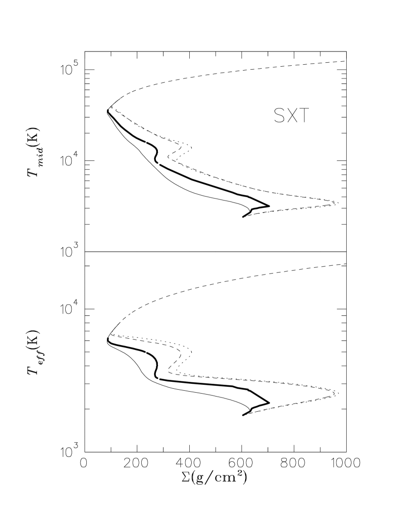
Figure 3: S-curves of SXT disks ($M_{WD}=10\,M_{\odot}$, $\log r\,{\rm cm}=10.5$) for different vertical energy transport models: $F_{all,damp}$ (thicker solid line), $F_{all,nodamp}$ (dotted line), $F_{rad}+F_{conv,MLT}$ (dashed line), and $F_{rad}+F_{turb}$ (solid line). All curves are based on the scaling law $\alpha=50(c_{s}/r/\Omega)^{3/2}$.

Figure 4: Fractional energy fluxes of SXT disks ($M_{WD}=10\,M_{\odot}$, $\log r\,{\rm cm}=10.5$) along the vertical direction $z$ for the same half-thickness $\log h\,{\rm cm}=8.33$ in the cases of damped convection (top panel) and MLT convection (bottom panel). $F_{rad}/F_{total}$, $F_{conv}/F_{total}$, and $F_{turb}/F_{total}$ are denoted by a solid line, a dashed line, and a dotted line respectively.

Figure 5: S-curves of SXT disks around a $10\,M_{\odot}$ central black hole at $\log r\,{\rm cm}=9$ and $9.75$ for different vertical energy transport models: $F_{all,damp}$ (thicker solid line), $F_{all,nodamp}$ (dotted line), $F_{rad}+F_{conv,MLT}$ (dashed line), and $F_{rad}+F_{turb}$ (solid line). All curves are based on the scaling law $\alpha=50(c_{s}/r/\Omega)^{3/2}$.. We also show the aspect ratio of convective cells, $A^{1/2}$ and the strength of convection $\Gamma_{c}/\Omega$ in the middle of the convective region as a function of $T_{eff}$. The values of $A^{1/2}$ and $\Gamma_{c}/\Omega$ are the maximum and minimum values for a given $T_{eff}$.

Figure 6: S-curves of AGN disks ($M_{WD}=10^{8}\,M_{\odot}$, $\log r\,{\rm cm}=15.5$) for different vertical energy transports: $F_{all,damp}$ (thicker solid line), $F_{all,nodamp}$ (dotted line), $F_{rad}+F_{conv,MLT}$ (dashed line), and $F_{rad}+F_{turb}$ (solid line). The line composed of crosses denotes the S-curve for the flux model $F_{rad}+F_{conv,MLT}$ with a shorter mixing-length $\log\,(\Lambda/\lambda_{p})=-0.5$. All curves are based on the scaling law $\alpha=50(c_{s}/r/\Omega)^{3/2}$.

Figure 7: Fractional energy fluxes of AGN disks ($M_{WD}=10^{8}\,M_{\odot}$, $\log r\,{\rm cm}=15.5$) along the vertical direction $z$ for the same half-thickness $\log h\,{\rm cm}=12.58$ in the cases of damped convection (top panel) and MLT convection (bottom panel). $F_{rad}/F_{total}$, $F_{conv}/F_{total}$, and $F_{turb}/F_{total}$ are denoted by solid line, dashed line, and dotted line respectively.

Figure 8: Effective temperature $T_{eff}$ vs. the ratio of self-gravity to central object gravity $g_{self}/g_{central}$ for AGN models whose total vertical energy flux is $F_{all,damp}$.

Figure 9: Maximum values of convective fluxes and vertical ranges of damped convection are plotted with respect to effective temperature $T_{eff}$ for different systems. The dashed lines denote $F_{conv,max}/F_{all,nodamp}$, where $F_{conv,max}$ is the maximum MLT convective flux at a given $T_{eff}$. The solid lines denote $F_{conv,max}/F_{all,damp}$, where $F_{conv,max}$ is the maximum damped convective flux at a given $T_{eff}$. The vertical ranges (scaled with $h$) of damped convection are indicated by the dotted lines.

Figure 10: Effective temperature vs. the ratio of radial to vertical length $\sqrt{A}$ of damped convection for different systems. The solid and dotted lines represent the maximal and minimal values of $\sqrt{A}$ respectively at a given $T_{eff}$. No solutions exist on the left side of dotted lines for weak convection (i.e. smaller $\sqrt{A}$) as a result of strong damping.

Figure 11: Influence of metal abundance on the S-curves around $\Sigma{max}$ for MLT convection and turbulent mixing in DN (top panel), SXT (middle panel), and AGN (bottom panel) disks. Solid lines indicate the curves $F_{tot}=F_{rad}+F_{conv,MLT}$ with metals. Dashed-dotted lines indicate the curves $F_{tot}=F_{rad}+F_{conv,MLT}$ without metals. Dashed lines denote the curves $F_{tot}=F_{rad}+F_{turb}$ with metals. And dotted lines denote the curves $F_{tot}=F_{rad}+F_{turb}$ without metals.

Figure 12: S-curves of DN disks ($M_{WD}=M_{\odot}$, $\log\,r({\rm cm})=9$) associated with different energy transports for $\alpha=0.1$ around $\Sigma_{min}$: $F_{all,damp}$ (thicker solid line), $F_{all,nodamp}$ (dotted line), $F_{rad}+F_{conv,MLT}$ (dashed line), and $F_{rad}+F_{turb}$ (solid line).

References

- Alexander, Johnson, and Rypma (1983) Alexander, D. R., Johnson, H. R., and Rypma, R. L. 1983, ApJ, 272, 773
- Armitage, Livio, and Pringle (1996) Armitage, P. J., Livio, M., and Pringle, J. E. 1996, ApJ, 457, 332
- Balbus and Hawley (1991) Balbus, S., and Hawley, J.F. 1991, ApJ, 376, 214
- Balbus and Hawley (1998) Balbus, S., and Hawley, J. F. 1998, Rev. Mod. Phys., 70, 1
- Batchelor (1950) Batchelor, G.K. 1950, Proc. Roy. Phil. Lond., A201, 405
- Blaes and Balbus (1994) Blaes, O. M., and Balbus, S. A. 1994, ApJ, 421, 163
- Burrell (1997) Burrell, K.H. 1997, Phys. Plasmas, 4, 1499
- Cabot et. al. (1987) Cabot, W., Canuto, V. M., Hubickyj, O., & Pollack, J. B. 1987, Icarus, 69, 423
- Cannizzo (1992) Cannizzo, J. K. 1992, ApJ, 385, 94
- Cannizzo (1993) Cannizzo, J. K. 1993, in Accretion Disks in Compact Stellar Systems, ed. J. C. Wheeler (Singapore: World Scientific), p. 6
- Cannizzo (1994) Cannizzo, J. K. 1994, ApJ, 435, 389
- Cannizzo and Cameron (1988) Cannizzo, J. K., and Cameron, A. G. W. 1988, ApJ, 330, 327
- Cannizzo, Chen, and Livio (1995) Cannizzo, J. K., Chen, W., and Livio, M. 1995, ApJ, 454, 880
- Cannizzo and Wheeler (1984) Cannizzo, J. K., and Wheeler, J. C. 1984, ApJS, 55, 367
- Canuto and Hartke (1986) Canuto V. M., and Hartke, G. J. 1986, A&A, 168, 89
- Chandrasekhar, (1960) Chandrasekhar, S. 1960, Proc, Nat. Acad. Sci., 46, 253
- Chen, Shrader, and Livio (1997) Chen, W., Shrader, C. R., and Livio, M. 1997, ApJ, 491, 312
- Cox and Giuli (1968) Cox, J. P., and Giuli, R. T. 1968, Principles of Stellar Structure (New York: Gordon and Breach)
- Cox and Stewart (1969) Cox, A. N., and Stewart, J. N. 1969, Sci. Inf., Astr. Council, Acad. Sci. USSR, No. 15, p. 1.
- D’Alessio et. al. (1998) D’Alessio, P., Cantó, J., Calvet, N., and Lizano, S. 1998, ApJ, 500, 411
- Dubus et al. (1999) Dubus, G., La-Sota, J.P., Hameury, J.-M., and Charles, P.A. 1999, MNRAS, 302, 731
- Gammie (1997) Gammie, C.F. 1997, astro-ph/9712233
- Gammie and Menou (1998) Gammie, C.F., and Menou, K. 1998, ApJ, 492, L75
- Hameury et al. (1998) Hameury, J.-M., Menou, K., Dubus, G., Lasota, J.-P., and Hure, J.-M. 1998, MNRAS, 298, 1048
- Hawley and Balbus (1992) Hawley, J., and Balbus, S. 1992, ApJ, 400, 595
- Hawley, Balbus and Winters (1999) Hawley, J.F., Balbus, S.A., and Winters, W.F. 1999, ApJ, 518, 394
- Honma (1996) Honma, F. 1996, PASJ, 48, 77
- Iben (1963) Iben, Jr., I. 1995, ApJ, 138, 452
- Kazantsev (1967) Kazantsev, A.P. 1967, JETP, 53, 1806
- King & Ritter (1998) King, A.R., and Ritter, H. 1998, MNRAS, 293, 42
- Lin and Shields (1986) Lin, D. N. C., and Shields, G. A. 1986, ApJ, 305, 28
- Livio and Spruit (1991) Livio, M., and Spruit, H. C. 1991, A&A, 252, 189
- Ludwig, Meyer-Hofmeister, and Ritter (1994) Ludwig, K., Meyer-Hofmeister, E., and Ritter, H. 1994, A&A, 290, 473
- Maeder (1995) Maeder, A. 1995, A&A, 299, 84
- Maeder and Meynet (1996) Maeder, A., and Meynet G. 1995, A&A, 313, 140
- Menou, Hameury, & Stehle (1999) Menou, K., Hameury, J.-M., and Stehle, R. 1999, MNRAS, in press
- Meyer and Meyer-Hofmeister (1982) Meyer, F., and Meyer-Hofmeister E. 1982, A&A, 106, 34
- Mineshige (1988) Mineshige, S. 1988, A&A, 190, 72
- Mineshige and Osaki (1983) Mineshige, S., and Osaki, Y. 1983, PASJ, 35, 377
- Narayan, McClintock, and Yi (1996) Narayan, R., McClintock, J. E., and Yi, I. 1996, ApJ, 457, 821
- Osaki (1996) Osaki, Y. 1996, PASP, 108, 39
- Pojmański (1986) Pojmański, G. 1986, Acta Astr., 36, 69
- Pollack, McKay and Christofferson (1985) Pollack, J. B., McKay, C. P., and Christofferson, B. M. 1985, Icarus, 64, 471
- Ruden, Papaloizou, and Lin (1988) Ruden, S. P., Papaloizou, J. C. B., & Lin, D. N. C. 1988, ApJ, 329, 739
- Rüdiger et. al. (1988) Rüdiger, C., Elstner, D., and Tschäpe, R., 1988, Acta Astr., 38, 299
- Sakimoto and Coroniti (1981) Sakimoto , P. J., and Coroniti, F. V., 1981, ApJ, 247, 19
- Schittkowski (1985) Schittkowski, K. 1985/86, Annals of Operations Research, 5, 4850
- Shakura and Sunyaev (1973) Shakura, N. I., and Sunyaev, R. A. 1973, A&A, 24, 337
- Smak (1984) Smak, J. 1984, Acta Astr., 34, 161
- Spellucci (1998) Spellucci, P. 1998, URL: http://plato.la.asu.edu/guide.html
- Speziale, Sarkar and Gatski (1991) Speziale, C.G., Sarkar, S., and Gatski, T.B. 1991, J. Fluid Mech., 227, 245
- Speziale and Gatski (1997) Speziale, C.G., Sarkar, S., and Gatski, T.B. 1997, J. Fluid Mech., 344, 155
- Stone et. al. (1996) Stone, J., Hawley, J.F., Gammie, C.F., and Balbus, S.A. 1996, ApJ, 463, 656
- Talon and Zahn (1997) Talon, S., and Zahn, J.-P. 1997, A&A, 317, 749
- Velikhov (1959) Velikhov, E. P. 1959, Soviet Phys. - JETP, 36, 1398
- Vishniac (1993) Vishniac, E. T. 1993, in Accretion Disks in Compact Stellar Systems, ed. J. C. Wheeler (Singapore: World Scientific), p. 41
- Vishniac (1997) Vishniac, E. T. 1997, ApJ, 482, 414
- Vishniac (1998) Vishniac, E.T. 1998, Proceedings of the 1997 Maryland Meeting, in press (available as astro-ph/9802232)
- Vishniac (1999) Vishniac, E.T. 1999, proceedings of the 1998 Chapman Conference on Magnetic Helicity, ed. A. Pevtsov (AGU: New York)
- Vishniac and Diamond (1992) Vishniac, E. T., and Diamond, P. H. 1992, ApJ, 398, 561
- Vishniac and Brandenburg (1997) Vishniac, E.T., and Brandenburg, A. 1997, ApJ, 475, 263
- Vishniac and Wheeler (1996) Vishniac, E. T., and Wheeler, J. C. 1996, ApJ, 471, 921
- Wood et al. 1986, (1989) Wood, J. H., Horne, K., Berriman, G., & Wade, R. A. 1989, ApJ, 341, 974
- Wood et al. 1986, (1989) Wood, J. H., Horne, K., Berriman, G., Wade, R. A., & O’Donoghue, D. 1986, MNRAS, 219, 629
- Zahn (1992) Zahn, J.-P., 1992, A&A, 265, 115