The Distribution of High and Low Redshift Type Ia Supernovae

Abstract

The distribution of high redshift Type Ia supernovae (SNe Ia) with respect to projected distance from the center of the host galaxy is studied and compared to the distribution of local SNe. The distribution of high–$z$ SNe Ia is found to be similar to the local sample of SNe Ia discovered with CCDs, but different than the sample discovered photographically. This is shown to be due to the Shaw effect. These results have implications for the use of SNe Ia to determine cosmological parameters if the local sample of supernovae used to calibrate the light curve decline relationships is drawn from a sample discovered photographically. A K–S test shows that the probability that the high redshift SNe of the Supernova Cosmology Project are drawn from the same distribution as the low redshift calibrators of Riess et al.  is 0.1%. This is a potential problem because photographically discovered SNe are preferentially discovered farther away from the galaxy nucleus, where SNe show a lower scatter in absolute magnitude, and are on average 0.3 magnitudes fainter than SNe located closer to the center of their host galaxy. This raises questions about whether or not the calibration SNe sample the full range of parameters potentially present in high redshift SNe Ia. The limited data available suggest that the calibration process is adequate; however, it would be preferable if high redshift SNe and the low redshift SNe used to calibrate them were drawn from the same sample, as subtle differences may be important. Data are also presented which suggest that the seeming anti-Malmquist trend noticed by Tammann et al. (1996, 1998) for SNe Ia in galaxies with Cepheid distances may be due to the location of the SNe in their host galaxies.

1 Introduction

Statistical studies of SNe give us information about the Universe on all scales. They give us clues about the progenitors of SNe (impacting stellar evolution), reveal the galactic SN rate (influencing galaxy evolution), and are being used to determine cosmological parameters (the evolution of the Universe). For all of these tasks, obtaining an unbiased sample of SNe, and thus fully understanding the selection effects involved in SN discovery, is essential. This work will focus on selection effects that may affect the use of SNe Ia as distance indicators, so only SNe Ia are discussed.

1.1 SNe as Standard Candles

All SNe Ia are thought to be caused by the thermonuclear explosions of carbon–oxygen (CO) white dwarfs in binary systems (Hoyle & Fowler 1960). Their low dispersion in absolute magnitude allows them to be used as “calibrated candles,” though some care must be exercised if they are to be used in this capacity. The first Hubble diagram constructed from Type I SNe by Kowal (1968) revealed a dispersion in photographic magnitude of $\sim$0.6 mag. Barbon et al. (1973) noted that Type I SNe were not a homogeneous class — some light curves declined faster than others. Pskovskii (1977,1984) then suggested that the light curve decline rate is correlated with the luminosity of SNe. Slower declining SNe Ia are intrinsically more luminous than those with fast-declining light curves. The separation of the Type Ib (Elias et al. 1985) and Ic subclasses (Wheeler & Harkness 1986), and the shift to modern CCD detectors allowed Phillips (1993) to establish a decline rate parameter, $\Delta m_{15}(B)$, the decline in blue magnitude from maximum after 15 days, and to conclusively show that it was correlated with the absolute magnitudes of SNe at maximum. In a study of 29 SNe Ia, Hamuy et al. (1996) have shown that correcting the absolute magnitudes at maximum in this way reduces the dispersion from $\sigma$= 0.38, 0.26, 0.19 to $\sigma$= 0.17, 0.14, 0.13 in the B, V, and I bands respectively. Another approach, the Multicolor Light Curve Shape (MLCS) technique (Riess, Press, & Kirshner, 1996), makes use of the entire shape of the light curve in various colors to reduce the dispersion at maximum light to $\sigma\simeq 0.15$ magnitudes. These results have given promise that SNe Ia may be used as calibrated candles to determine large scale motions of the local group (Riess, Press, & Kirshner, 1995), and the cosmological parameters H₀, $\Omega$, and $\Lambda$ (Goobar & Perlmutter 1995). Several searches have already discovered a combined number of $\sim$ 100 high redshift SNe ($0.3\leq z\leq 1.0$) for this purpose (Riess et al. 1998, Perlmutter et al. 1999), with the remarkable suggestion that $\Lambda$ is finite and positive.

1.2 The Shaw Effect

Shaw (1979) first characterized a selection effect in supernova searches that had long been suspected. On photographic plates, supernovae are less frequently discovered in the often overexposed central regions of distant galaxies. Shaw estimated that $\sim$50% of supernovae are lost within the central 8 kpc of galaxies beyond 150 Mpc. The effect is reduced for closer galaxies. A correction factor must be introduced to account for this effect when determining SN rates. Bartunov et al. (1992) and Cappellaro et al. (1993, 1997) find that supernova searches experience the Shaw effect to varying degrees, so the correction factor for each search can be different.

To quantify the Shaw effect, one must compare supernovae discovered photographically to an “unbiased” sample. This has been attempted with varying degrees of success, but so far each comparison group has had problems. Out of necessity, Shaw (1979), in his own words, made the “unwarranted” assumption that supernovae discovered in galaxies closer than 33 Mpc were free from this effect. Prior to this, the loss of SNe in the inner regions of galaxies was estimated by extrapolation of the SN rate in the outer regions of galaxies to a central peak following the light distribution (Johnson & MacLeod 1963; McCarthy, 1974; Barbon et al. 1975). Bartunov et al. (1992) confirmed Shaw’s suspicion that even the nearby sample is not free from bias. Bartunov et al. and Cappellaro et al. used combined data from visual and CCD searches as the control group.

1.3 Differences in SN Properties with Galactocentric Distance

As pointed out by Wang, Höflich & Wheeler (1997, hereafter WHW), SN properties appear to vary with projected galactocentric distance (PGD). Using data from 40 local well-studied SNe Ia, WHW find that SNe located more than 7.5 kpc from the centers of galaxies show 3–4 times lower scatter in maximum brightness than those projected within that radius. (Note that the projected distance is the minimum distance the SN can be from the center of the galaxy. Many events at small PGD are actually located far from the center of the host galaxy.) A reduction of scatter with PGD is also apparent in the $B_{\rm max}-V_{\rm max}$ colors of the SNe. In the absence of corrections for light curve shape, SNe at higher projected galactocentric distance are a more homogeneous group and should be better for use as distance indicators. The reddest and bluest, brightest and dimmest SNe are located near the galactic center, so extinction alone cannot explain the higher scatter in this region. Indeed, Riess et al. (1999) find that scatter still remains in these relationships when the SNe are corrected for extinction using the MLCS technique. The scatter is reduced after the SNe are corrected for the light curve decline relationship, leaving no apparent trend with PGD.

As suggested by WHW and confirmed by Riess et al. (1999), SNe in the outer regions of galaxies show systematic differences in luminosity with respect to those with smaller projected separations from the host center. After correcting for extinction, Riess et al. find that SNe at distances of 10 kpc or more from the centers of their host galaxies are dimmer by about 0.3 mag than the mean of those (projected) inside 10 kpc. Riess et al. also note that this effect may be related to one pointed out by Hamuy et al. (1996) and Branch et al. (1996) — SNe in early-type hosts tend to be dimmer. At high PGD, the sample is dominated by SNe in elliptical host galaxies. Possible sources for the variation in SN properties with projected distance (if intrinsic) include metallicity gradients within the galaxy or differences in progenitor systems between the disks and bulges.

2 The sample

Five groups of SNe Ia were studied in this work - the local sample discovered with CCDs, the local SNe discovered photographically, the high redshift SNe discovered by the Supernova Cosmology Project, the local SNe used to calibrate the brightness of the high–$z$ SNe, and eleven very local supernovae discovered in galaxies with Cepheid distances that are used to tie the SN distance scale to the Cepheid distance scale.

The IAU Circular “List of Supernovae” web page was used to determine the initial sample. The Asiago Supernova Catalog (Barbon et al. 1989) was used to provide missing data and the recession velocities of the host galaxies. Any recession velocities not in the Asiago catalog were taken from the NASA/IPAC Extragalactic Database (NED). The sample was divided into high and low redshift at $z=0.3$.

The SNe were retained if they met the following criteria:

• Type Ia

• Projected offset of SN from center of host galaxy is known

• Recession velocity or distance to host galaxy is known

• Method of discovery is known

Distances to galaxies with recession velocities greater than 3000 km s^-1 were computed using H₀= 65 km s^-1 Mpc^-1. For galaxies under 3000 km s^-1 distances were taken from Tully (1985) and scaled to H₀= 65.

The distances to high redshift SNe were calculated using the angular size distance for the $\Lambda=0$ model:

$$D=\frac{2c}{H_{0}}\left(\frac{(2-\Omega+\Omega z)-(2-\Omega)\sqrt{1+\Omega z}}{\Omega^{2}(1+z)^{2}}\right)$$

(Fukugita et al. 1992) assuming $H_{0}=65$, $\Omega=0.2$.

The method of discovery (photographic, visual, CCD) was not listed in any database, so this information was obtained directly from the IAU Circulars reporting the discovery of each SN.

When SNe are very near to the center of the host galaxy, positions are sometimes reported as “very close” to the center, and no separation in arcseconds is given. Four supernovae fell into this category, SNe 1994U, 1996am, 1997dg, and 1998ci. All are in the sample of local SNe Ia discovered with CCDs. Removing these SNe from the sample would have biased the results, so they were retained and assigned zero offset from the center of the galaxy. Presumably these SNe were located so close to the center of their host galaxy that the offset can be considered negligible.

The high redshift SNe used were primarily those discovered by the Supernova Cosmology Project. Finding charts were downloaded from the group’s website. Because the charts were in postscript format, galactocentric separations had to be estimated visually, so each separation measurement has some degree of uncertainty associated with it, especially for SNe close to the cores of galaxies. Several of the SNe do have galactocentric separations reported in the circulars. Whenever possible, these numbers were used.

The smallest group consists of eleven SNe that have been discovered in galaxies with Cepheid distances. These supernovae are important for the determination of the Hubble constant, as they set the absolute distance scale.

The final group of SNe studied was the group of 27 local SNe used by Riess et al. 1998 to calibrate the MLCS and $\Delta m_{15}(B)$ techniques. The Supernova Cosmology Project used only 18 local calibrators, nearly a subset of the Riess et al. sample, so are not studied separately here. Both sets are drawn from the Calán/Tololo SN survey (see Phillips et al. 1999), so they were discovered by the same methods, and should have nearly identical properties. This amounts to comparing the high redshift SNe (mostly) from one team with the low redshift SNe of another team, but this is not expected to be a problem. The two groups use similar discovery techniques for the high redshift SNe and nearly identical SNe for the low redshift calibrators, so the conclusions of this paper should be applicable to both groups. We have chosen the only data available at high redshift, and the most statistically significant sample of low redshift calibrators to study in this paper, and these happen to be from different research groups.

3 Results

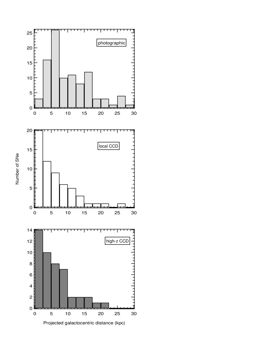
Figure 1: The distribution of three samples of SNe Ia: those discovered photographically, local SNe discovered with CCDs, and high–$z$ SNe discovered with CCDs.

Histograms of the distribution of SNe with respect to PGD were generated for SNe discovered with CCDs locally, at high redshift, and SNe discovered photographically. These are presented in Fig. 1. There are not enough data points in the Riess et al. calibration sample to generate a meaningful histogram.

SNe are presented with respect to raw PGD. Care must be taken in the interpretation of such data because it can be misleading and is impossible to properly normalize with the data available. As one travels farther out in PGD, the area swept out by each histogram bin increases. Corrections for this effect are not posible because there is no way to know the true distance of each SN from the center of its host galaxy (only the projected distance is known). Also, the inclination is not known for each galaxy, and the areal calibration would be different for face-on spirals than it would be for edge-on spirals. It is noteworthy that SNe Ia discovered on CCDs are found in greater numbers in bins covering the smallest area — those closer to the center of the galaxy.

Additional unremovable forms of bias are present in the data. The projection of a three dimensional galaxy onto the two dimensional sky can cause interesting effects. High PGDs are more likely to be representative of true galactocentric distances. Consider an edge on spiral galaxy. SNe at high PGD are confined to a smaller range of distances perpendicular to the plane of the sky than SNe observed near the center of the galaxy. SNe with zero PGD may actually have a very high true galactocentric distance.

The smaller size and faintness of galaxies at high redshift make them more susceptible to random errors in determining the PGD. These random errors can act like systematic errors because they tend to work in the same direction. SNe near the centers of galaxies may appear to have a larger PGD due to noise. It is far more unlikely for noise to lower a PGD.

Human selection effects may also play a role in biasing the data. SNe near the centers of galaxies may be neglected at high redshift due to the difficulty of obtaining spectra of SNe contaminated with galaxy light.

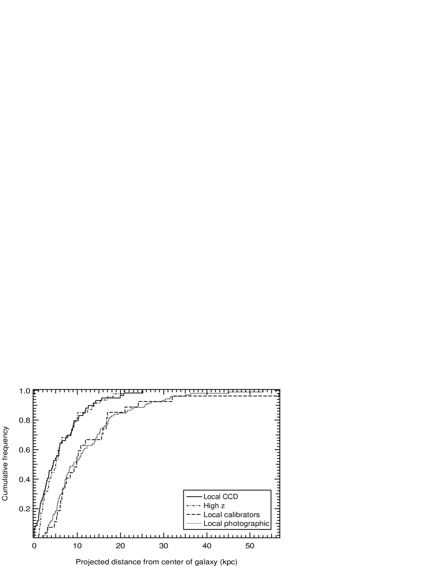
Figure 2: The cumulative frequency of SNe Ia versus projected separation from the galactic nucleus.

Each data set was sorted in order of increasing PGD and cumulative distributions were generated, given in Figure 2. The left axis can be interpreted as the fraction of SNe in each sample that are projected interior to a given galactocentric distance. The greatest vertical distance between two cumulative distribution curves is the Kolmogorov-Smirnov (K–S) statistic D (Press et al. 1988). This is used to determine the K–S probability that two samples were drawn from the same distribution.

A K–S test was done on each of the four data sets with respect to each other and is presented in Table 1. The null hypothesis is that the two samples in each comparison were drawn from the same distribution. The numbers in Table 1 are the percent chance that the null hypothesis is true. A few special cases deserve comment.

The probability that the sample of SNe discovered on photographic plates is drawn from the same distribution as the sample of SNe discovered on CCDs (at comparable redshifts, $z<0.3$) is $4\times 10^{-5}$. As can be seen in Fig. 2, the difference is due to the lack of SNe discovered near the centers of galaxies on photographic plates, i.e. the Shaw Effect.

In contrast, the K–S probability that local SNe discovered with CCDs and high–$z$ SNe discovered with CCDs are drawn from the same distribution is 58%. This number is probably artificially low due to the uncertainties in the positions of several local SNe very near the centers of galaxies as mentioned above. Indeed, when the sample is restricted to SNe with PGD of 3 kpc or greater, the corresponding K–S probability increases to 74%. Note that according to K–S statistics, these probabilities approaching unity do not mean the distributions are the same, but that they cannot be differentiated.

Figures 1 and 2 illustrate another selection effect caused by the differences between CCD and photographic discovery of SNe. SNe in the outer regions of galaxies that are discovered by photographic means tend to be missed or omitted in CCD searches. This is usually assumed to be due to the fact that CCDs have a smaller field of view and may not sample the outer regions of galaxies. One would thus expect that high–$z$ SNe would not show this effect, because their host galaxies have a smaller apparent angular diameter. Figure 2 shows that the high–$z$ SNe presented in this study do show such a cutoff. This is probably due to the limited number of data points. Assuming SNe Ia arise from an exponential disk population with a scale length of 5.0 kpc, the probablility of discovering a SN farther than 21 kpc from the center of the galaxy is 1.5%. In a sample of 49 SNe, it is not surprising that no SNe are seen at a galactocentric distance greater than 21 kpc. In addition, at high redshift, SNe at large PGD may not be followed up (Clocchiatti, private communication).

The sample of local SNe used to calibrate the high–$z$ SNe of Riess et al. (1998) was compared to the other groups of SNe. Twenty-four of twenty-seven of these local calibrators (89%) were discovered photographically, and are also members of the sample of photographically discovered SNe studied in this paper. Figure 2 shows that the cumulative distribution of the local calibrators used by Riess et al.  matches one expected from a photographic sample. The K–S test gives the probability that the photographic sample and the Riess et al. calibrators are drawn from the same distribution as 94%. This number is given only for completeness, as the K–S test is not meaningful for significantly overlapping samples.

The most striking result is that the K–S test gives a probability of only $10^{-3}$ that the high–$z$ SNe are drawn from the same distribution as the local SNe used to calibrate them. The calibrators tend to be located farther from the centers of galaxies than the high–$z$ sample, so again the Shaw effect is largely to blame. The implications for the use of these SNe as standard candles are discussed below.

Tables 2 and 3 reveal another subtle selection bias brought about by the Shaw Effect that has previously been overlooked. It is well known that SN discoveries in nearby galaxies are relatively unaffected by the Shaw Effect due to their large angular size. Of the eleven SNe with Cepheid distances, ten were located at a PGD of less than 10 kpc (see Table 2). This is particularly troubling given the findings of WHW and Riess et al. (1999) that SNe within this distance are on average 0.3 magnitudes brighter than supernovae located farther from the centers of their host galaxies. The SNe that tie the distant SNe to the Cepheid distance scale are drawn from a sample of potentially overluminous supernovae. This has implications for the determination of H₀  as discussed in the next section.

In summary, the closest SNe (which are used to tie all other SNe to the Cepheid distance scale) are free from the Shaw Effect, but biased toward overluminous SNe. The intermediate SNe were largely discovered photographically, and are quite susceptible to the Shaw Effect. As a result, these supernovae (which are used as calibrators to train the MLCS technique and derive the light curve–decline relationship) are biased toward underluminous SNe. Finally, the high–$z$ SNe were discovered with CCDs and are relatively immune to the Shaw Effect. These results can easily be seen in Table 3. The median PGD for the photographic sample is 9.1 kpc, compared to a median of only 4.4 kpc for the CCD sample. The very local Cepheid calibrators have the smallest median PGD at only 3.2 kpc.

4 Conclusions

Recently Hatano et al. (1998) proposed an alternative explanation for the Shaw Effect. They speculated that the Shaw Effect in Type II and Ibc SNe arises because extinction causes these supernovae to appear dim when projected onto the centers of galaxies, and dimmer SNe are harder to detect with increasing distance. Their model does not predict a paucity of SNe Ia near the centers of galaxies, and they were unconvinced that there is a real observational deficit of SNe Ia in this region. The data presented here confirm that the Shaw effect does indeed exist for photographically discovered Type Ia supernovae. These data support the traditional interpretation of the Shaw Effect — SNe are missed due to saturation of galaxy cores on photographic plates.

These data provide an estimate for the magnitude of the Shaw Effect in SNe Ia. If we assume the CCD sample is free from bias (the smaller FOV bias is small as noted earlier), then 80% of SNe should be located within a PGD of 10 kpc (see Figure 2 and Table 3). In the photographic sample, 50 SNe have a PGD $\geq$ 10 kpc. If this represents 20% of the sample, then the total sample should be $\sim$ 250 SNe; however, there are only 105 SNe in the sample, so $\sim$ 145 (58%) are missing. Thus nearly 60% of SNe Ia are lost near the centers of galaxies on photographic plates due to the Shaw Effect. This is striking because it is higher than most estimates of the Shaw Effect for all SNe, despite the fact that SNe Ia are $\sim$ 1.5 times brighter on average than SNe II. This is the key piece of evidence that saturation (not extinction) is to blame for the paucity of SNe. It would be very interesting to do a relative comparison of the samples of Type II and Type b/c SNe discovered with CCD’s compared to Type Ia SNe to explore the relative concentrations toward the centers of galaxies.

The high redshift SN sample appears to be relatively free from selection bias in terms of separation from the center of the galaxy. These SNe were discovered with CCDs and show a distribution with respect to galactocentric distance similar to that of local SNe discovered with CCDs. We find no evidence that high–$z$ SNe are selectively discovered farther from the centers of galaxies.

The high–$z$ SN studies may be sensitive to selection effects. According to Riess et al. (1998), “we must continue to be wary of subtle selection effects that might bias the comparison of SNe Ia near and far.” They also add, “It is unclear whether a photographic search selects SNe Ia with different parameters or environments than a CCD search or how this could affect a comparison of samples. Future work on quantifying the selection criteria of the samples is needed.”

This raises a potential area of concern when using SNe Ia as distance indicators. The light curve decline – absolute magnitude relationship used to calibrate the brightness of high–$z$ SNe is derived mainly from local SNe discovered photographically, as is the case in Riess et al. (1998) and Perlmutter et al. (1999). These SNe tend to be located farther from the centers of galaxies than the SNe in the high–$z$ sample. The calibrators are thus drawn from a sample subject to selection bias that is both more uniform in luminosity and dimmer than average. Because the calibrators are likely more homogeneous as a group than the high–$z$ SNe, they may not be able to effectively correct for the light curve decline relationship over all of parameter space.

This work has shown that there are issues of selection bias to be considered, but how much these issues affect the use of SNe Ia as distance indicators remains unclear. Fig. 6c of Riess et al. (1999) shows that after SN magnitudes are corrected for light curve shape using the MLCS technique there is no apparent trend of absolute V magnitude at maximumn with PGD. In this case the calibration process seems to work adequately. No data is available to indicate how well other calibration methods, particularly $\Delta m_{15}(B)$, (used by Riess et al. 1998 in addition to MLCS) and the stretch factor method (used by Perlmutter et al. 1999), can compensate for changes in the absolute magnitudes of SNe with PGD. Since these calibration methods all rely on the same principle — using the shape of the light curve to correct for variations in luminosity — one might expect that all will work similarly. It is also not known how the calibration process affects the trend reported by WHW of increased scatter in the colors of SNe at maximum light with decreasing PGD. Future work is needed to assure that all methods of calibration of SNe Ia can remove trends with PGD in all bandpasses. No previous studies have found significant problems with the calibration process, so the results of Riess et al. (1998), and Perlmutter et al. (1999) do not appear to be at risk due to selection bias. Evidence for a local void (Zehavi et al. 1998), already marginal, may be more sensitive to subtle effects.

The PGD-magnitude effect when combined with the Shaw effect may explain several unusual findings reported recently. Tammann et al. (1996) and Tammann (1998) noted that after SNe luminosities are corrected via a light curve decline relationship, local SNe with Cepheid distances are brighter than average, and this is the opposite than one would expect from a magnitude limited sample (the farthest SNe should be brightest because we could not see the faint ones). This discrepency has been used to argue that there is a problem with light curve decline relationships. From the result presented here – that ten of eleven SNe with Cepheid distances have PGD $<10$ kpc – these SNe can be expected to be overluminous.

Two of the SNe with reported Cepheid distances, 1980N and 1992A, do not actually have a Cepheid distance determined to their host galaxies, but are members of the Fornax cluster, for which a Cepheid distance of $(m-M)_{0}=31.35$ is available by assuming that the galaxy NGC 1365 is a member of the cluster (Madore et al. 1999). These two SNe appear to be too dim, by 0.3 mag, compared to the Calán/Tololo sample of SNe Ia, leading Suntzeff et al. (1999) to speculate that NGC 1365 may be foreground to Fornax by 0.3 mag. Interestingly, these SNe have the highest PGD of the SNe in Cepheid galaxies, at 20.0 and 9.3 kpc, respectively, both outside the distance WHW identify as the cutoff beyond which SNe Ia are seen to be 0.3 mag dimmer on average. A possible explanation for the faintness of SN 1980N and SN 1992A is their location in their host galaxies, rather than an error in the distance to Fornax. It should also be noted, however, that Saha et al. (1999) derive a distance modulus to NGC 1316 of $(m-M)_{0}=31.84$, by assuming that SN 1980N in NGC 1316 is similar to SN 1989B, which would make SN 1980N too bright.

The fact that the Cepheid calibrators are drawn from a potentially overluminous sample of SNe is troubling. This could affect determinations of the Hubble constant that rely on using these very local SNe for calibration purposes. The fact that different biases operate on different distance scales calls into question the variation of H₀ with distance reported by Tammann (1998), as no second parameter correction was used.

More data is needed on the galactic radial distribution of high and low redshift SNe. Given the discovery rate of high–$z$ SNe and the fact that they presumably do not face the discovery bias related to the small size of a CCD relative to the host galaxy, the statistics of the intrinsic distribution of high–$z$ SNe may soon be known more precisely than those of the low redshift sample.

In an ideal world, the luminosity of high–$z$ SNe would only be calibrated with SNe discovered using CCDs. That is not possible at the present time, so early work indicating that light curve decline – absolute magnitude relationships can effectively remove the effects of selection bias should be continued and strengthened.

Table 1: K–S Probabilities

	Calib	Hi-z	CCD
Photo	94	0.008	0.004
Calib	$\cdots$	0.1	0.05
Hi-z	$\cdots$	$\cdots$	58

Table 2: Projected Galactocentric Distances of Cepheid Calibrators

SN	Host	D	PGD
		(Mpc)	(kpc)
1895B	NGC 5253	4.3	0.7
1972E	NGC 5253	4.3	2.5
1937C	IC 4182	5.4	1.3
1981B	NGC 4536	16.6	4.1
1960F	NGC 4496	16.8	3.0
1990N	NGC 4639	25.5	8.0
1989B	NGC3627	11.4	2.8
1998bu	NGC 3368	11.9	3.2
1974G	NGC 4414	19.14	5.8
1992A	NGC 1380	18.6	9.3
1980N	NGC 1316	18.6	20.0

Table 3: Median PGD and SNe within 10 kpc

Sample	Median	NPGD<10	Ntot	%PGD<10
	(kpc)
Local CCD	4.4	47	59	80%
Local Photo	9.1	55	105	52%
High–z	4.6	41	47	87%
Riess Calibrators	9.9	15	27	56%
Cepheid Calibrators	3.2	10	11	91%