No evidence for a ‘redshift cut-off’ for the most powerful classical double radio sources

Abstract

We use three samples (3CRR, 6CE and 6C*) to investigate the radio luminosity function (RLF) for the ‘most powerful’ low-frequency selected radio sources. We find that the data are well fitted by a model with a constant co-moving space density at high redshift as well as by one with a declining co-moving space density above some particular redshift. This behaviour is very similar to that inferred for steep-spectrum radio quasars by Willott et al (1998) in line with the expectations of Unified Schemes. We conclude that there is as yet no evidence for a ‘redshift cut-off’ in the co-moving space densities of powerful classical double radio sources, and rule out a cut-off at $z\stackrel{{\scriptstyle<}}{{{}_{\sim}}}2.5$.

¹Astrophysics, Department of Physics, Keble Road, Oxford, OX1 3RH.
²Instituto de Astrofísica de Canarias, C/ Via Lactea s/n, 38200 La Laguna, Tenerife, Spain
³Department of Physics and Astronomy, University of Wales College of Cardiff, P.O. Box 913, Cardiff, CF2 3YB

1. Introduction

It is well-known that the (co-moving) space densities of the rarest, most powerful quasars and radio galaxies were much higher at epochs corresponding to $z\sim 2$ than they are now (Longair 1966). The behaviour of the space density beyond these redshifts is the subject of this paper. Dunlop & Peacock (1990) found evidence for a ‘redshift cut-off’ (a decline in the co-moving space density) in the distribution of flat-spectrum radio sources over the redshift range $2-4$. Through failing to find any flat-spectrum radio quasars at $z>5$ in a large ($\approx\,$40 per cent of the sky) survey, Shaver et al (1996, hereafter SH96) argued for an order-of-magnitude drop in space density between $z\sim 2.5$ and $z\sim 6$, for this class of object. As emphasised by SH96, the crucial advantage of any radio-selected survey is that with sufficient optical follow-up, it can be made free of optical selection effects, such as increasing dust obscuration at high redshift. It is chiefly for this reason that the work of SH96 provides the most convincing evidence to date for the existence of an intrinsic decline in the co-moving space density of any galaxy class at very high redshift.

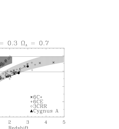
Figure 1.: $L_{151}-z$ plane for the three samples used in our analysis. 3CRR (diamonds; Laing, Riley & Longair 1983), 6CE (crosses; Eales et al 1997), 6C* (stars; Blundell et al 1998; Jarvis et al in prep.) and Cygnus-A (filled triangle). The filled circles represent the three 6C* sources with upper redshift limits and the associated arrows show the paths of the possible redshifts and luminosities for these sources. The area between the horizontal lines is the region which contains the ‘most powerful’ sources according to our definition. The dark grey region shows the approximate $L_{151}-z$ plane coverage of the 3CRR sample ($10.9\>{\rm Jy}\leq S_{178}\leq 80.0\>{\rm Jy}$, spectral index, $\alpha=0.5$) and the light grey region the 6C* sample ($0.96\>{\rm Jy}\leq S_{151}\leq 2.0\>{\rm Jy}$, with $\alpha=0.98$ and $\alpha=1.5$ for the lower and upper fluxes, respectively). Note the area between the two shaded regions contains no sources, this is the area which corresponds to the absence of a flux-limited sample between the 6CE ($S_{151}\leq 3.93\>$Jy) and 3CRR ($S_{178}\geq 10.9\>$Jy) samples.

2. Modelling the RLF

We adopt a parameterisation of the RLF which is separable in 151-MHz luminosity $L_{151}$ and redshift $z$ with a single power-law in $L_{151}$ of the form $(L/L_{\circ})^{-\beta}$. We consider two cosmologies $\Omega_{\rm M}=1$, $\Omega_{\Lambda}=0$ (cosmology I) and $\Omega_{\rm M}=0.3$, $\Omega_{\Lambda}=0.7$ (cosmology II). Model A parameterises the redshift distribution as a single power-law of the form $(1+z)^{n}$. For model B the redshift distribution is parameterised as a Gaussian, giving an overall expression for the co-moving space density of $\rho=\rho_{\circ}(L/L_{\circ})^{-\beta}\exp-\{(z-z_{\circ})/\sqrt{2}\,z_{1}\}^{2}$ where $\rho_{\circ}$ and $\beta$ are the normalising term and power-law exponent respectively, $z_{\circ}$ is the Gaussian peak redshift and $z_{1}$ is the characteristic width of the Gaussian. Model C is described by the same model up to $z_{\circ}$ beyond which it becomes constant.

3. Results and Discussion

For sources in the top-decade in luminosity of the $L_{151}-z$ plane (Fig. 1) our parametric fitting and likelihood analysis of model radio luminosity functions (Table 1) show that the data are inconsistent with a $(1+z)^{n}$ power-law in redshift (Model A), but are well fitted by both models B and C. These models are shown in Fig.$\,2$ in the form of a log$\,N$ / log$\,S$ plot. We conclude that although the relative likelihood for model B is $2.5$ times larger than for model C, this is not statistically significant enough to distinguish between the two models with any confidence. This uncertainty is further compounded by the effects of assuming a mean spectral index in the model fitting. This result is in very close agreement with the RLFs for radio loud quasars modelled by Willott et al (1998) and various studies of AGN at optical (Irwin et al 1991) and X-ray (Hasinger et al 1998) wavelengths.

This is in apparent contradiction to the findings of SH96 for flat-spectrum quasars. If the relationship between the flat- and steep-spectrum populations is as described by unification models of AGN then we might expect to see similar evolution in the two populations. Thus to determine the co-moving space density of radio sources at high-redshift, an understanding of the spectral index trends, $K-$corrections and associated selection effects must first be achieved.

Fig.$\,2$ also illustrates the contribution of powerful sources at high redshift to the total source count in a low-frequency survey. We see that even for the no cut-off model (Model C) the fractional contribution is very small. This may render the location of the redshift cut-off virtually impossible to determine until the selection effects associated with radio surveys are fully understood.

Model	Cosmology	$\log_{10}(\rho_{\circ})$	$\beta$	$n$	$z_{\circ}$	$z_{1}$	$P_{KS}$	$\mathcal{L}_{R}$
A	I	$-9.04$	1.61	1.19	—–	—–	0.10	$10^{-5}$
B	I	$-7.94$	1.98	—–	2.59	0.94	0.33	1
C	I	$-8.18$	1.95	—–	1.69	0.54	0.41	0.4
A	II	$-9.45$	1.63	0.85	—–	—–	0.12	$10^{-5}$
B	II	$-8.51$	2.00	—–	2.60	0.96	0.36	1
C	II	$-8.78$	1.93	—–	1.67	0.53	0.41	0.3

Table 1.: Best-fit parameters for the model RLFs, described in the text. $P_{KS}$ is the 2-D Kolmogorov-Smirnov probability (a value above $0.2$ signifies a reasonable fit to the data) and $\mathcal{L}_{R}$ is the likelihood relative to model B.
Errors for model B (cosmology I): $\Delta\log_{10}(\rho_{\circ})=0.17$, $\Delta\beta=0.2$, $\Delta z_{\circ}=0.10$, $\Delta z_{1}=0.17$, for 68% confidence regions.

Figure 2.: For cosmology II we show the areal density of the most powerful radio sources as a function of 151-MHz flux density $S_{151}\,/\;$Jy in comparison with the total source count. The 6CE source count (squares) is reproduced from Hales, Baldwin & Warner (1988) and the 7C source count (diamonds) from McGilchrist et al (1990). The 3C source (stars) count was inferred from the revised 3CR sample of Laing, Riley & Longair (1983). The large open star represents the 6C* data (note that this is a lower-limit due to spectral index and angular size selection in this filtered sample); the open circle the 6CE sample; the inverted triangles the 3 bins representing the 3CRR sample. The solid horizontal lines show the $S_{151}$ range of each sample. The lower panel shows the percentage of the total source count contributed by each model. Models A, B and C are represented by the dotted, dashed and solid lines respectively.

References

Blundell K.M., Rawlings S., Eales S.A., Taylor G.B., Bradley A.D., 1998, MNRAS, 295, 265

Dunlop, J.S. & Peacock, J.A., 1990, MNRAS, 247, 19

Eales S.A., Rawlings, S., Law-Green, D., Cotter, G., Lacy, M., 1997, MNRAS, 291, 593

Hales, S.E.G., Baldwin, J.E. & Warner, P.J., 1988, MNRAS, 234, 919

Hasinger, G., 1998, Astron. Nachr., 319, 37

Irwin, M., McMahon, R. & Hazard, C., 1991, in The Space Distribution of Quasars, ed. Crampton, ASPCS 21, 117

Laing, R.A., Riley, J.M. & Longair, M.S., 1983, MNRAS, 204,151

Longair, M.S., 1966, MNRAS, 133, 421

McGilchrist M.M., Baldwin, J.E., Riley, J.M., Titterington, D.J., Waldram, E.M., Warner, P.J., 1990, MNRAS, 246, 110

Shaver, P.A., Wall, J.V., Kellermann, K.I., Jackson, C.A., Hawkins, M.R.S., 1996, Nature, 384, 439

Willott, C.J., Rawlings, S., Blundell, K.M., Lacy M., 1998, MNRAS, 300, 625