Perturbations of spherical stellar systems during fly-by encounters

Abstract

We study the internal response of a galaxy to an unbound encounter and present a survey of orbital parameters covering typical encounters in different galactic environments. Overall, we conclude that relatively weak encounters by low-mass interloping galaxies can cause observable distortions in the primaries. The resulting asymmetries may persist long after the interloper is evident.

We focus our attention on the production of structure in dark halos and in cluster ellipticals. Any distortion produced in a dark halo can distort the embedded stellar disk, possibly leading to the formation of lopsided and warped disks. We show that distant encounters with pericenters in the outer regions of a halo can excite strong and persistent features in the inner regions. Features excited in an elliptical are directly observable and we predict that asymmetries in the morphologies of these systems can be produced by relatively small perturbers. For example, a fly-by on an orbit with pericenter equal to the half-mass radius of the primary system and velocity of 200 km/s (a value typical for groups) can result in a significant dipole distortion for perturbers with mass as small as 5% of primary’s mass.

We use these detailed results to predict the distribution of the $A$ parameter defined by Abraham et al. (sensitive to lopsidedness) and the shift between the center of mass of the primary system and the position of the peak of density for a range of environments. We find that high-density, low-velocity dispersion environments are more likely to host galaxies with significant asymmetries. Our distribution for the $A$ parameter is in good agreement with the range spanned by the observed values for local galaxy clusters and for distant galaxies in the Medium Deep Survey and in the Hubble Deep Field. Assuming that primordial galaxies were located in dense environments with previrialized low velocity dispersions, our conclusions are consistent with the observational results showing a systematic trend for galaxies at larger redshifts to be more asymmetric than local galaxies.

Finally, we propose a generalized asymmetry parameter $A(r)$ which provides detailed information on the radial structure of the asymmetry produced by the mechanism explored in our work.

1. Introduction

Galaxy interactions are likely to play a key role in determining the morphology and the structural properties of galaxies and in driving evolution at all epochs and in widely-varying environments. The importance of environmental conditions on the properties of populations of galaxies has been recognized for a long time (Hubble & Humason 1931) and observational studies have now firmly established relationships between the relative abundance of galaxies of different morphological types and the density of the environment (see e.g. Dressler 1980, Dressler et al. 1997), their location in clusters (Oemler 1974) as well as the evolution of the morphology of galaxies in clusters at different epochs (Butcher & Oemler 1978, 1984). In particular, the ratio of early to late-type galaxies has been shown to be an increasing function of density and a decreasing function of the distance from the center of a cluster. In addition, HST observations show that the relative number of spirals to elliptical and S0 galaxies tend to increase in distant clusters, pointing to a time evolution of the morphology of galaxies from spirals to ellipticals (see e.g. Dressler et al. 1994a, 1994b, Couch et al. 1998). Altogether, these results suggest that environmental disturbances due to interactions with other galaxies and with a cluster tidal field can lead to dramatic changes in the structure of galaxies.

Simulations have explored strong encounters and mergers. Our recent work suggests that relatively weak encounters can give rise to significant asymmetries as well. To study weaker galaxy interactions and quantify their importance, we compute the response of a spherical stellar system to the perturbation induced by another system during a fly-by, focusing our attention on the morphology and the persistence of the distortions produced during the encounter. The range of orbital parameters considered encompasses the typical environmental conditions for field galaxies, for galaxies in groups and in clusters. Our perturbative solution for these distortions provides quantitative and qualitative predictions in low to moderate amplitude that are difficult to reach by simulation. This approach nicely reveals the underlying dynamics without being masked or swamped by n-body fluctuation noise. On the other hand, numerical feasibility restricts the complexity of possible geometries and the perturbative assumption limits its validity for large amplitudes.

Our investigation is relevant for galactic dark halos or for spheroidal galaxies over a range of environments. We explore the possibility that the halo distortions produced during a fly-by could in turn lead to a significant and observable distortion in an embedded stellar disk (see e.g. Weinberg 1995, 1998b, Murali & Tremaine 1998, Murali 1998). In particular the deformations produced in a dark halo during an encounter could be one of the culprits for distorted morphologies like those observed in lopsided and warped galactic disks (see e.g. Richter & Sancisi 1994, Zaritsky & Rix 1997, Rudnick & Rix 1998, Swaters et al. 1998, Haynes et al. 1998, Kornreich, Haynes & Lovelace 1998). As recently shown by Weinberg (1995, 1998b), this could be the case for the Milky Way in which the deformations induced in the dark halo by the Magellanic Clouds could be responsible for the observed warp in the Galactic disk. In a recent investigation, Reshetnikov & Combes (1998, 1999) have found that about 40% of a sample of 540 galaxies have warped planes and their analysis revealed that warped galaxies tend to be located in denser environments supporting a scenario in which interactions would play an important role in the formation of warps.

Distortions of spheroidal galaxies are directly observable. Our results show that in low velocity dispersion and dense environments, where low-velocity close encounters are more likely to occur, even low-mass perturbers can lead to significant asymmetries in the primary galaxy. Recent morphological studies of both local and very distant galaxies have yielded comparisons of the frequencies of systems with distorted morphologies in different environments and at different distances (see e.g. Zepf & Whitmore 1993, Mendes de Oliveira & Hickson 1994, Abraham et al. 1996a,1996b, van den Bergh et al. 1996, Naim, Ratnatunga & Griffiths 1997, Brinchmann et al. 1998, Marleau & Simard 1998, Conselice & Bershady 1998, Conselice & Gallagher 1999). On the theoretical side, the efforts have been largely concentrated on numerical $N$-body simulations aimed at investigating the fate and the evolution of merging galaxies (see e.g. Barnes & Hernquist 1992, Barnes 1998 and references therein) and the distortions and the morphological alterations produced in galaxies in clusters and groups by the ensemble of “tidal shocks” with other members (Moore et al. 1996, 1998). This mechanism can drive the evolution of spiral galaxies into spheroidal systems and it is a strong candidate explanation for the difference in the relative number of spiral to elliptical galaxies in clusters at different redshifts.

The plan of the paper is the following. In §2 we outline the method adopted for this investigation while the mathematical details are described in the Appendix. In §3 we show the results obtained for initial conditions typical of galactic dark halos and their dependence on the orbital parameters of the perturber. In §4 initial conditions relevant for spheroidal galaxies and a survey of orbital parameters of the perturber typical of different environments are considered. Overall, our results quantify the relationship between the interaction rate for the environment and the probability of observing irregular morphologies, aiding interpretation of any trend in the fraction of asymmetric galaxies at different redshifts. This latter aspect is of particular interest as data on the morphology of distant galaxies are now available from HST observations in the Hubble Deep Field and in the Medium Deep Survey projects (Abraham et al. 1996a, 1996b). In order to facilitate the comparison of our theoretical results with observational data, we will quantify the distortions produced by means of the asymmetry parameter $A$ (Abraham et al. 1996a) which has been determined for a number of local and distant galaxies. We will also introduce a generalized asymmetry parameter $A(r)$ which will provide an important information on the radial structure of the asymmetry produced by the mechanism we have considered and which will allow to test the theory presented here. The main conclusions are summarized and discussed in §5.

2. Method

This section outlines the perturbative solution of the collisionless Boltzmann equation used to predict the dynamical response of galaxies to interactions. Additional mathematical detail is presented in the Appendix.

The linear perturbation theory used here has been applied in the past both to investigate the collisionless stability of stellar disks (Kalnajs 1977) and of spherical stellar systems (Polyachenko & Shukhman 1981, Palmer & Papaloizou 1987, Bertin & Pegoraro 1989, Saha 1991, Weinberg 1991, Bertin et al. 1994; see also Palmer 1994 and references therein) and to study the response of a galaxy to perturbations induced by satellite companions (Weinberg 1989, 1995, 1998b). This method is numerically intensive but it avoids the problems of n-body simulations due to the finite number of particles which can introduce spurious noise effects (see Weinberg 1998a) and it guarantees the resolution of resonances that lead to the excitation of patterns in the primary system. With too few particles, for example, noise can cause orbital energies and angular momenta to drift on a time scale shorter than the pattern speed of the global response of interest. This eliminates the possibility of observing this structure in the simulation. No doubt, real galaxies are not smooth and inherent fluctuations may be important to their evolution. However, many millions of n-body particles are required to approach the estimates of natural amplitudes (Nelson & Tremaine 1996, Weinberg 1998a).

We compute the perturbation induced on a spherical stellar system by a point mass perturber with mass $m$ on a rectilinear trajectory with pericenter $p$. The response of the primary system will be determined by the simultaneous solution of the linearized collisionless Boltzmann and Poisson’s equations,

$${\partial f_{1}\over\partial t}+{\partial f_{1}\over\partial{\bf w}}{\partial H_{0}\over\partial{\bf I}}-{\partial f_{0}\over\partial{\bf I}}{\partial H_{1}\over\partial{\bf w}}=0,$$ (1)

$$\nabla^{2}\Phi_{1}=4\pi G\rho_{1},$$ (2)

where the subscript $0$ denotes the equilibrium quantities, subscript $1$ denotes the first order perturbation of the distribution function $f$, the Hamiltonian $H$, and the potential $\Phi$. The Boltzmann equation has been written in terms of action-angle variables $\bf{I},\bf{w}$. The perturbed potential, $\Phi_{1}$, is the sum of the tidal potential due to the perturber, $\Phi_{p}$, and the gravitational potential of the response to the perturbation, $\Phi_{resp}$, and $\rho_{1}=\rho_{1}^{p}+\rho_{1}^{resp}$. The coupled Boltzmann-Poisson equations lead to an integrodifferential equation for the potential. This can be solved by performing a Fourier transform in the angle variables, a Laplace transform in the time variable and expanding the perturbed quantities in terms of spherical harmonics and of a bi-orthogonal density-potential basis functions for the angular and the radial parts respectively. The integrodifferential equation is then reduced to an algebraic equation for the vector of coefficients of the expansion of the response potential and density, a,

$${\bf a}={\bf R}({\bf a}+{\bf b}).$$ (3)

The matrix R contains the time dependence of the perturbation and the equilibrium properties of the perturbed system and b is the vector of the coefficients of the expansion of the external perturbing potential.

It is clear from equation (3) that the self-consistent response of the perturbed system is determined both by the perturbation applied by the external perturber and by the reaction of the system to its own response to this perturbation. In general, an additional contribution to the total response comes from excitation of the discrete damped modes of the primary system besides the effects of the perturber and the self-gravity of the distorted primary. The differences in the mathematical structure of these two contributions are illustrated in the Appendix. The transient response due to the discrete damped modes can have a strong effect on the amplitude of the response (cf. §3) and it is particularly important when the modes are weakly damped with damping timescales longer than the fly-by timescale. In this case, the discrete damped modes produce long-lived features which completely determine the amplitude and the structure of the response long after the pericenter passage of the perturber. Once the above algebraic equation has been solved, the calculation of response potential and density is straightforward

$$\Phi_{1}^{resp} = {1\over 2}\sum_{lm}\left[Y_{lm}(\theta,\phi)\sum_{i}a_{i}^{lm}u_{i}^{lm}(r)\right.$$ (4)

$$\left.+Y_{lm}^{*}(\theta,\phi)\sum_{i}a_{i}^{lm*}u_{i}^{lm}(r)\right]$$

$$\rho_{1}^{resp} = {1\over 2}\sum_{lm}\left[Y_{lm}(\theta,\phi)\sum_{i}a_{i}^{lm}d_{i}^{lm}(r)\right.$$ (5)

$$\left.+Y_{lm}^{*}(\theta,\phi)\sum_{i}a_{i}^{lm*}d_{i}^{lm}(r)\right]$$

where $d_{i}$ and $u_{i}$ are the bi-orthogonal density-potential basis function and $Y_{lm}(\theta,\phi)$ are the spherical harmonics.

3. Perturbation of dark halos

Features excited in the halo can give rise to visible distortions in an embedded disk even though dark halo perturbations are not directly observable. While several other processes could be responsible for the observed distorted morphologies of stellar disks (see e.g. Sellwood & Merritt 1994, Levine & Sparke 1998, Bertin & Mark 1980, Nelson & Tremaine 1995), the role played by a distorted galactic dark halo in exciting peculiar features in disks has been advanced for the case of an interaction of a galaxy with a satellite companion by Weinberg (1995,1998b) and applied to the case of the Milky Way-Magellanic Cloud system. Halo deformations leading to morphological and kinematical lopsidedness has been invoked by Swaters et al. (1998) in an analysis of two kinematically lopsided spiral galaxies (DDO 9, NGC 4395). The ubiquity of Magellanic-class dwarf companions of normal spirals (e.g. Zaritsky & White 1994 and Zaritsky et al. 1997) suggests that such interactions may be important sources of structure. Unbound encounters can have similar effect as we will illustrate here.

Our standard dark halo model is an isotropic King model with a dimensionless central potential $W_{0}=3.0$ (concentration $c=0.67$) a total mass $M=6\times 10^{11}M_{\odot}$ and a total radius $R_{t}=200$ kpc. These values are appropriate for the Galactic halo (see e.g. Kochanek 1996) and together with a standard exponential disk results in a fair fit to the observed rotation curve. Given the primary model, the perturber’s velocity $V$ and pericenter $p$ determine the structure of the response to the perturbation. The amplitude of the response scales with the mass of the perturber.

Table 1 summarizes the values of $V$ and $p$ explored here along with the corresponding values of the ratio of the pericenter to the half-mass radius of the primary system, $p/R_{h}$, and the ratio of the characteristic frequency of the motion of the perturber to the circular frequency at the edge of the primary system, $\Omega\equiv V/p\sqrt{R_{t}^{3}/GM}$. All the cases considered here correspond to fly-bys in which part of the orbit passes through the halo; external encounters are likely to produce weaker distortions and will be considered later in §3.3. The values of $V$ considered are chosen to cover a typical range of relative encounter velocities in the field, groups and clusters. In order to clearly assess the importance of weakly damped modes, we consider the evolution of the response both with and without their effect for all the cases listed in Table 1.

Table 1
Orbital parameters for the fly-by
encounters with a low-concentration
primary system
$V$ (km/s)	$p$ (kpc)	$p/R_{h}$	$\Omega$
200	53.6	1.0	6.45
500	53.6	1.0	16.1
1000	53.6	1.0	32.3
200	107.2	2.0	3.23
500	107.2	2.0	8.1
1000	107.2	2.0	16.1

For cases that include the weakly damped modes, we must first determine their natural frequencies. We used the method adopted in Weinberg (1994): the determinant of the dispersion matrix ${\bf D}(s)$ (see Appendix for its definition) is evaluated on a grid of values of $s$ in the upper ($Re(s)>0$) complex plane where the determinant is defined and then rational functions are used to perform the analytical continuation to the lower complex plane where the zeros of the determinant corresponding to damped modes are located. Rational function fits of the elements of the dispersion matrix have been adopted also for the calculation of the residue of the inverse of the dispersion matrix necessary to include the effects of damped modes in the response coefficients (see eq. A16). The characteristic damping times for the most weakly damped modes, $\tau_{l}$, are $\tau_{1}/t_{dyn}\simeq 150$ and $\tau_{2}/t_{dyn}\simeq 30$ for the dipole and the quadrupole mode respectively, where $t_{dyn}$ is the dynamical time of the primary system defined at the half-mass radius, $t_{dyn}\equiv\pi\sqrt{R_{h}^{3}/2GM}$.

3.1. Importance of damped modes

Figure 1 shows the evolution of the energy in the perturbation, $E_{p}$, as a function of $t/t_{dyn}$ (Fig.1a-b) and as a function of the position angle of the perturber $\Theta(t)$ (Fig.1c-d) without the effects of the damped modes. We normalize to the total background energy of the primary system $E_{back}\equiv\nu GM^{2}/R_{t}$ ($\nu=-0.78$ for a King $W_{0}=3$ model).

For a given value of the pericenter, the peak of the response occurs after the closest approach. The faster the perturber, the larger the value of the position angle and the more distant the perturber location when the response of the primary system reaches its peak.

Figure 1.— Run of energy in the perturbation with time and with the position angle of the perturber for fly-bys with $p/R_{h}=1.0$ (a) and (c) and $p/R_{h}=2.0$ (b) and (d). The three curves shown in each frame correspond (from the upper to the lower curve) to $V=200$ km/s, $V=500$ km/s, $V=1000$ km/s. $E_{back}$ is the total background energy of the primary system and $t_{dyn}$ is the half-mass dynamical time. Pericenter occurs at $t=0$.

The strength of response increases as the velocity of the perturber decreases. In Figure 2 we have plotted the maximum value of $E_{p}$ as a function of the velocity of the perturber for the two values of $p$ investigated. The response amplitude is large when the characteristic angular frequency, $V/p$, is in low-order resonance with primary orbital frequencies.

Figure 3 and Figure 4 show the same plots shown in Figure 1 and Figure 2 but with the effects of the discrete weakly damped modes taken into account. The maximum values of $E_{p}$ are about two orders of magnitude larger than those reached when the effects of damped modes are not included while the dependence of the peak of $E_{p}$ on the velocity of the perturber and on the pericenter of its orbit are similar to each other in the two cases. The inclusion of the damped modes is critical to the persistence and the strength of the perturbation.

A simple empirical function of the form $K/V^{\alpha}$ can be used to obtain a satisfactory fit of the curves shown in Figure 2 and Figure 4. These relations can be used to predict ensemble properties (see §3.4 for an example). Table 2 summarizes the values of the parameters $K$ and $\alpha$ for the best fits for all the cases investigated and shown in Figure 2 and Figure 4.

Table 2
Best fit parameters for the scaling
of $\max(0.1M/m)^{2}E_{p}/E_{back}$ with the
relative velocity of encounters
Parameters	$K$	$\alpha$
$p/R_{h}=1.0$, no-damped	0.005	1.41
$p/R_{h}=2.0$, no-damped	0.002	1.33
$p/R_{h}=1.0$, with damped	1.0	1.96
$p/R_{h}=2.0$, with damped	0.5	1.9
The scaling of $\max(0.1M/m)^{2}E_{p}/E_{back}$ with the relative
velocity of encounters, $V$, has been fitted using the function
$f(V)={K\over(V(\hbox{km/s})/200)^{\alpha}}$.

The scalings obtained will not extend to the very low-velocity regime where they would lead to a divergence of the energy associated to the response. In the limit of very slow encounters we expect the energy of the response to increase more slowly and eventually to converge to a constant value (see Murali & Tremaine 1998 for an investigation of the response of galactic halos to adiabatic perturbations).

Figure 2.— Maximum value of the energy in the perturbation, $E_{p}$, as a function of the perturber velocity $V$. The upper curve corresponds to fly-bys with $p/R_{h}=1.0$ and the lower curve to fly-bys with $p/R_{h}=2.0$.

Figure 5 illustrates the differences between the response with and without the damped modes by separately showing the energy in the dipole and quadrupole components for $V=500$ km/s and $p/R_{h}=1.0$. As expected, the dipole response is significantly stronger than that of quadrupole. The inclusion of the damped modes leads to a much longer and stronger dipole response, while producing no significant difference in the quadrupole response. Such long-lived features may explain the numerous cases of galaxies with distorted morphologies but without any apparent interacting system in their vicinities (e.g. Richter & Sancisi 1994). For example, for a system with mass and radius equal to those of our fiducial system ($M=6\times 10^{11}M_{\odot}$, $R=200$ kpc), the damping time of the dipole mode ($\tau_{1}=5\times 10^{10}$ yrs) is longer the Hubble time and any perturbation excited in a dark halo during a fly-by as well as its effect on an embedded disk will persist well after the encounter.

Figure 3.— Same as Fig. 1a-d but including the effects of weakly damped modes.

Figure 4.— Same as Fig. 2 but including the effects of weakly damped modes.

3.2. Structure of response

Contour plots in Figures 6 and 7 describe the density perturbation in the orbital plane for the dipole (upper panels) and quadrupole (lower panels) responses without and with the damped modes, respectively.

Figure 5.— Time evolution of the perturbation energy for a fly-by with $V=500$ km/s, $p/R_{h}=1.0$. Two cases with (solid lines) and without (dashed lines) damped modes are shown for the dipole response (upper two curves) and quadrupole response (lower two curves).

These cases have $V=200$ km/s and $p/R_{h}=1.0$ and show the response of the primary galaxy at three different points of the perturber trajectory. A lag between the orientation of the wake and the position angle of the perturber is evident for all velocities. This lag is a consequence of angular momentum transfer between the wake and the perturber and tends to zero only when there is no resonance affecting the response of the primary system . Physically, resonant momentum exchange viewed at the orbit level has a corresponding view as a global response: the global response must lag the perturber in order to apply the torque responsible for the exchange.

Figures 8a and 8b show the ratio, $R_{p}/R_{h}$, of the radial position of the peak of the density of the perturbation, $R_{p}$, to the half-mass radius, $R_{h}$, as a function of the position angle of the perturber without the effects of weakly damped modes for $V=200$ km/s and $p/R_{h}=1.0,2.0$ (Fig.8a) and for $p/R_{h}=1.0$ and $V=200,500,1000$ km/s (Fig.8b).

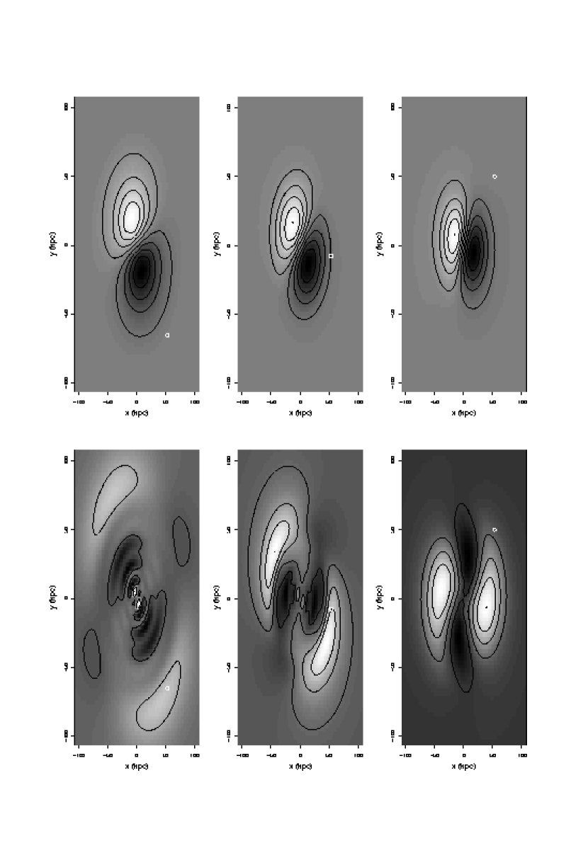
Figure 6.— Density distortion of the primary galaxy at three phases of the fly-by with $V=200$ km/s and $p/R_{h}=1.0$ without the effects due to the damped modes. Upper panels show the dipole response; lower panels show the quadrupole response. The white dot shows the position of the perturber. White and black regions correspond to overdensity and underdensity respectively.

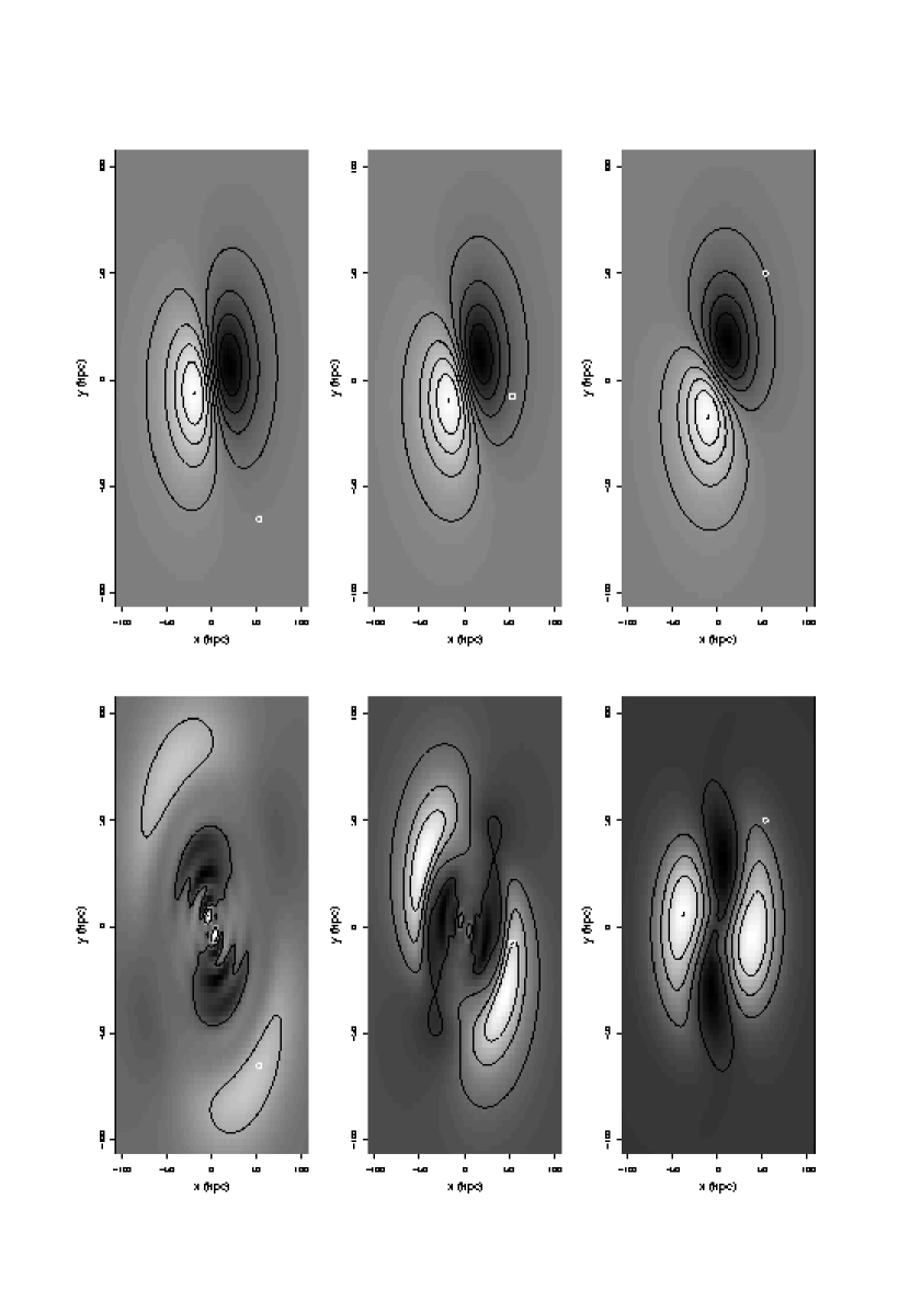
Figure 7.— Same as Fig. 6 but including the effects of weakly damped modes.

The evolution of $R_{p}/R_{h}$ is only weakly dependent on the velocity of the perturber and on the pericenter of the orbit of the perturber. The perturbation is efficiently transmitted to the inner parts of the primary system and the peak of the density of the perturbation is located at $0.3\hbox{ \hbox to0.0pt{\raise 1.82986pt\hbox{$<$}\hss}\lower 2.79857pt\hbox{$\sim$} }(R_{p}/R_{h})\hbox{ \hbox to0.0pt{\raise 1.82986pt\hbox{$<$}\hss}\lower 2.79857pt\hbox{$\sim$} }0.4$ or in terms of the core radius, $R_{c}$, $0.4\hbox{ \hbox to0.0pt{\raise 1.82986pt\hbox{$<$}\hss}\lower 2.79857pt\hbox{$\sim$} }(R_{p}/R_{c})\hbox{ \hbox to0.0pt{\raise 1.82986pt\hbox{$<$}\hss}\lower 2.79857pt\hbox{$\sim$} }0.5$ (for almost the entire duration of the fly-by). The weak dependence of the response on perturber parameters is due to the dominant effect of the lowest-order point modes on the structure of the dispersion matrix elements. For an analogy, consider the similarity of bell’s ring under a variety of strikes. The strong oscillations of $R_{p}/R_{h}$ in the final phases of the fly-by are due to numerical difficulty in determining the density peak as the response weakens.

Figures 9a and 9b show the evolution of the maximum value of the density of the perturbation $\delta\rho_{max}$ (normalized to the central density of the equilibrium model) for the same cases shown in Figures 8a and 8b. The maximum response obtains for slower fly-bys (cf. Fig. 1) and, for a given value of $V$, $\delta\rho_{max}$ increases as $p$ decreases. Figures 8c and 8d and 9c and 9d show the same plots as in Figures 8a-b and Figures 9a-b for fly-bys including the weakly damped modes.

Figure 8.— Evolution of the ratio of the position of the peak of the density distortion to the half-mass radius of the primary galaxy as a function of the position angle of the perturber for the fly-bys with (a) $V=200$ km/s and $p/R_{H}=1.0$ (dashed line) and $p/R_{h}=2.0$ (solid line) and (b) for the flybys with $p/R_{h}=1.0$ and $V=200$ km/s (solid line), $V=500$ km/s (short dashed line) $V=1000$ km/s (long dashed line). (c) and (d) same as (a) and (b) but including the effects of weakly damped modes.

Figure 9.— Maximum value of the density distortion as function of the position angle for the fly-bys with (a) $V=200$ km/s and $p/R_{H}=1.0$ (dashed line) and $p/R_{h}=2.0$ (solid line) and for the flybys with (b) $p/R_{h}=1.0$ and $V=200$ km/s (solid line), $V=500$ km/s (short dashed line) $V=1000$ km/s (long dashed line).(c) and (d) same as (a) and (b) but including the effects of weakly damped modes.

The position of the peak of the density is similar to that obtained in the case without the weakly damped modes but there are evident differences in the time evolution of $R_{p}/R_{h}$ particularly at the beginning and at the end of the fly-by due to the persistence of the damped modes. The response is significantly stronger when the effects of the damped mode are included (compare Fig.9a-b with Fig.9c-d)

Figure 10.— Energy in the perturbation as a function of the orthogonal function indices. Upper panels (a-c) correspond to the fly-by and the phases shown in Fig.6; lower panels (d-f) correspond to the fly-by and the phases shown in Fig.7. Open circles and crosses show the energy in the dipole response and in the quadrupole response respectively. Each curve is normalized to the maximum value of $E_{p}(n)$ .

Figure 10 shows the energy in the perturbation for the first ten basis functions and indicates the distribution of energy with spatial scale. Plots shown in Figure 10 are for the same cases and phases shown in Figure 6 and Figure 7. Figure 10 confirms what is already qualitatively evident in Figure 6 and Figure 7: the energy in the dipole response is preferentially deposited on large scales and the quadrupole response energy deposited on relatively smaller scales. The typical scale represented by each index $n$ can be seen from the plots of Figure 11 which show the density basis functions for $l=1$.

Figure 11.— Density basis functions used to represent the perturbation density (see §2).

3.3. External encounters

External encounters, those with trajectories everywhere outside the primary, are more frequent in groups and clusters but less dramatic. For external encounters, the stronger dipole response corresponds to a simple shift of the center of mass of the system leaving the weaker quadrupole as dominant aspherical contribution. Here we briefly describe the features of externally excited responses.

Table 3 summarizes the characteristics of the fly-bys we have investigated. An external encounter has no intrinsic length scale and the frequency parameter $\Omega$ alone now determines the structure of the response. The Table reports the velocity of each fly-by assuming the pericenter to be equal to twice the total radius of the primary system (400 kpc) and the maximum values of the ratio of the energy in the perturbation to the total energy of the equilibrium model. This values scales as shown for other values.

Table 3
External fly-bys
$\Omega$	$V_{p=2R_{t}}$ (km/s)	$\max\left({1.0\over R_{t}/p}\right)^{6}\left({1.0\over m/M}\right)^{2}{E_{p}\over E_{back}}$
0.1	23	$1.3\times 10^{-3}$
0.5	115	$1.3\times 10^{-3}$
1.0	231	$7.0\times 10^{-4}$
2.5	578	$4.7\times 10^{-4}$
5.0	1150	$2.8\times 10^{-4}$
$V_{p=2R_{t}}$ is the relative velocity of the encounter for
the given value of $\Omega$ reported in the first column for
for $p=2R_{t}=400$ kpc.

One sees that the effects of external encounters with less massive perturbers are weak and they can not produce a significant deformation in the primary system. On the other hand, if the perturber is more massive than the perturbed system even external fly-bys can be very important in affecting the structure of a galaxy. For example, in order to have $\max(E_{p}/E_{back})\simeq 0.01$ for an encounter with $p=2R_{t}$ the ratio of the mass of the perturber to that of the perturbed must be $m/M\simeq 30$. These encounters are relevant for spiral galaxies in clusters where they can undergo frequent external encounters with more massive giant ellipticals. A recent investigation by Rubin et al. (1999) has shown that about half of a sample of 89 spirals in the Virgo cluster exhibit signs of kinematic disturbances in their rotation curves; according to that investigation disturbed galaxies are preferentially on radial orbits likely to cross the central regions of the clusters where such encounters are likely to occur.

The five panels of Figure 12 show the contour plots of the density of the response when $E_{p}/E_{back}$ reaches its maximum value. As described in §3.2, the response reaches its maximum strength at different phases of the orbit of the perturber depending on the value of $\Omega$: the larger the value of $\Omega$, the more distant the perturber is from the pericenter of its orbit when the response is maximum. As the characteristic frequency of the fly-by decreases and the perturbation tends to the adiabatic regime, individual resonances cease to be relevant in determining the structure of the response and the orientation of the wake aligns with the position of the perturber. Finally, we note that some features are present at small radii and these may cause visible distortions in an embedded disk.

Figure 12.— Density distortion of the primary galaxy when the perturbation energy is maximum. The three frames on the left correspond to fly-bys with (from the upper to the lower panel) frequencies $\Omega=0.1,~{}0.5,~{}1.0$; the two frames on the right are for the fly-bys with $\Omega=2.5,~{}5.0$. The straight solid line in each panel indicates the position angle of the perturber.

3.4. Summary and discussion: dark halos

We have investigated the response of a galactic dark halo to the perturbation induced by external and internal fly-bys. External fly-bys are effective when the mass of the perturber is larger than that of the primary system considered. For example, perturbations excited in spirals during external fly-bys with more massive giant ellipticals can play an important role in altering their structure and kinematics. Similarly, external encounters will produce significant structure in dwarfs in the neighborhood of normal spirals.

We have shown that the perturbation excited during an internal fly-by encounter can be efficiently transmitted to the inner regions of the halo where it can affect the structure of an embedded stellar disk. The halo distortions can be significant and persistent for typical dwarf interlopers. This may lead to distorted morphologies like those observed in warped and lopsided disks. The survey over different velocities and pericenter distances provides a quantitative measure of the expected importance of the process investigated in different environments.

For an overall indicator of the fraction of objects distorted as a result of fly-by encounters, we have calculated the mean value of the peak relative distortion for different environments,

$$\langle\max~{}(0.1M/m)^{2}{E_{p}/E_{back}}\rangle={\int{K\over V^{\alpha}}f(V)V^{2}dV\over\int f(V)V^{2}dV}$$ (6)

where $f(V)$ is the distribution of the relative velocities of encounters which we take equal to a Gaussian with dispersion $\sigma$. Figure 13 shows $\langle\max(0.1M/m)^{2}E_{p}/E_{back}\rangle$ as a function of $\sigma$ for the four scaling laws listed in Table 2.

Figure 13.— Mean value of $\max(0.1M/m)^{2}E_{p}/E_{back}$ assuming a Gaussian distribution of the relative velocity of encounters versus the dispersion, $\sigma$, of the distribution. Solid lines (upper line for $p/R_{h}=1$, lower line for $p/R_{h}=2.0$) are for runs including the effects damped modes; dashed lines are for runs without the effects of damped modes.

Generally, low velocity dispersion compact groups with number densities $n\sim 10^{2}\hbox{ Mpc}^{-3}$ and velocity dispersions $\sigma\sim 10^{2}$ km/s are dominated by low-velocity close encounters which lead to the strongest response in the perturbed galaxies; cluster of galaxies which are characterized by higher velocity dispersions ($\sigma\sim 10^{3}$ km/s) and lower number densities ($n\sim 10^{0}-10^{1}\hbox{ Mpc}^{-3}$) encounters are expected to produce less pronounced effects.

The effects of damped modes on the strength and the persistence of the features excited by the perturber are significant. In particular the persistence of the deformations due to the long-lived dipole mode may explain the origin of the numerous lopsided disks in field galaxies which have no apparent companion (see e.g. Richter & Sancisi 1994, Zaritsky & Rix 1997). We have separated the response due to damped modes in Figure 13 to highlight their importance, however, true physical response includes both. Damped modes may be artificially suppressed in n-body simulations with small particle number owing to fluctuation-induced orbital diffusion.

In the next section, we will focus our attention on elliptical galaxies modeled as high-concentration King models for which the effects of discrete modes have not been considered because they have much shorter damping times (Weinberg 1993) and thus are not as relevant as they are for dark halos .

4. Perturbation of cluster elliptical galaxies

Table 4
Orbital parameters for the fly-by
encounters with a high-concentration
primary system
$V$ (km/s)	$p$ (kpc)	$p/R_{h}$	$\Omega$
200	7.0	0.5	17.9
500	7.0	0.5	44.7
1000	7.0	0.5	89.5
200	14.0	1.0	8.9
500	14.0	1.0	22.4
1000	14.0	1.0	44.7
200	42.0	3.0	3.0
500	42.0	3.0	7.5
1000	42.0	3.0	14.9
200	97.8	7.0	1.28
500	97.8	7.0	3.2
1000	97.8	7.0	6.4

We will model the primary system by an isotropic King model with $W_{0}=7.0$ which has a concentration $c=1.53$ . We adopt typical mass, total radius and half-mass radius values for cluster elliptical galaxies: $M=10^{12}M_{\odot}$ and $R_{t}=120$ kpc, $R_{h}=14.0$ kpc. Table 4 summarizes the properties of our model grid (see Table 1 for parameter definitions). The overall approach and procedure otherwise follows that described in §3 with similar physical interpretation. §4.1 briefly presents the response diagnostics developed in §3, highlighting the differences between responses in the low- and high-concentration primaries. §4.2 explores observational diagnostics of the fly-by induced asymmetries and proposes a generalization of one of the standard observational asymmetry parameters to test the dynamical mechanism explored here.

4.1. Structure of response

Figure 14 shows the time evolution of the perturbation energy. As expected (cf. §3), the innermost fly-bys induce the strongest response and, for a given value of the pericenter, the response becomes weaker as the velocity of the perturber increases. The time evolution of $E_{p}$ is characterized by several peaks and a non-negligible amplitude even as $\Theta$ tends to $\pi/2$ and the perturber moves away from the primary galaxy. The persistence of these features well past the closest passage of the perturber may explain the origin of distorted morphology in galaxies without any close visible companion.

Figure 14.— Evolution of the perturbation energy as a function of time ($t=0$ is the time of passage of the perturber at the pericenter of its orbit) (a-c) and the position angle of the perturber (d-f). Panels (a) and (d) are for fly-bys with $V=200$ km/s, panels (b) and (e) for $V=500$ km/s, panels (c) and (f) for $V=1000$ km/s. In each panel the curves shown correspond to different values of the pericenter of the orbit of the perturber: $p/R_{h}=0.5$ (solid line), $p/R_{h}=1.0$ (dotted line), $p/R_{h}=3.0$ (dashed line), $p/R_{h}=7.0$ (long dashed line).

Figure 15 shows the evolution of $R_{p}/R_{h}$. The response is manifested well inside the primary galaxy and it affects the very inner regions of the system $0.05\hbox{ \hbox to0.0pt{\raise 1.82986pt\hbox{$<$}\hss}\lower 2.79857pt\hbox{$\sim$} }R_{p}/R_{h}\hbox{ \hbox to0.0pt{\raise 1.82986pt\hbox{$<$}\hss}\lower 2.79857pt\hbox{$\sim$} }0.15$ ($0.2\hbox{ \hbox to0.0pt{\raise 1.82986pt\hbox{$<$}\hss}\lower 2.79857pt\hbox{$\sim$} }R_{p}/R_{c}\hbox{ \hbox to0.0pt{\raise 1.82986pt\hbox{$<$}\hss}\lower 2.79857pt\hbox{$\sim$} }0.6$) even when the pericenter of the perturber is as large as $3R_{h}$ or $7R_{h}$. The value of $R_{p}$ is determined by the dominant resonances determining the structure of the response of the primary system. The larger dynamic range in primary profile enables excitation of high-order resonances between the characteristic frequency of the motion of the perturber and the frequencies of the orbital motion at smaller radii in the primary system. The rectilinear trajectory considered here provides continuum spectrum of frequencies that peaks at approximately $V/p$.

Figure 15.— Evolution of the position of the peak density distortion as a function of the position angle for the fly-bys with $V=200$ km/s (a), $V=500$ km/s (b) and $V=1000$ km/s (c). In each panel the four curves correspond to different values of the pericenter of perturber: $p/R_{h}=0.5$ (solid line), $p/R_{h}=1.0$ (dotted line), $p/R_{h}=3.0$ (dashed line), $p/R_{h}=7.0$ (long dashed line).

We found that $R_{p}/R_{c}$ is roughly constant for all the fly-bys investigated. This agrees with the results obtained by Weinberg (1994) in his analysis of the structure of weakly damped modes in isotropic King models. This implies that more concentrated models are more efficient in transmitting to the inner regions the perturbation excited during a fly-by (compare Fig.8 with Fig.15).

Figure 16 shows the density distortions for a fly-by with $V=200$ and $p/R_{h}=1.0$ at three different phases of the orbit of the perturber. As in previous cases, the maximum response occurs well inside the primary system and the perturbation is efficiently transmitted to the inner regions of the system far inside the orbital pericenter.

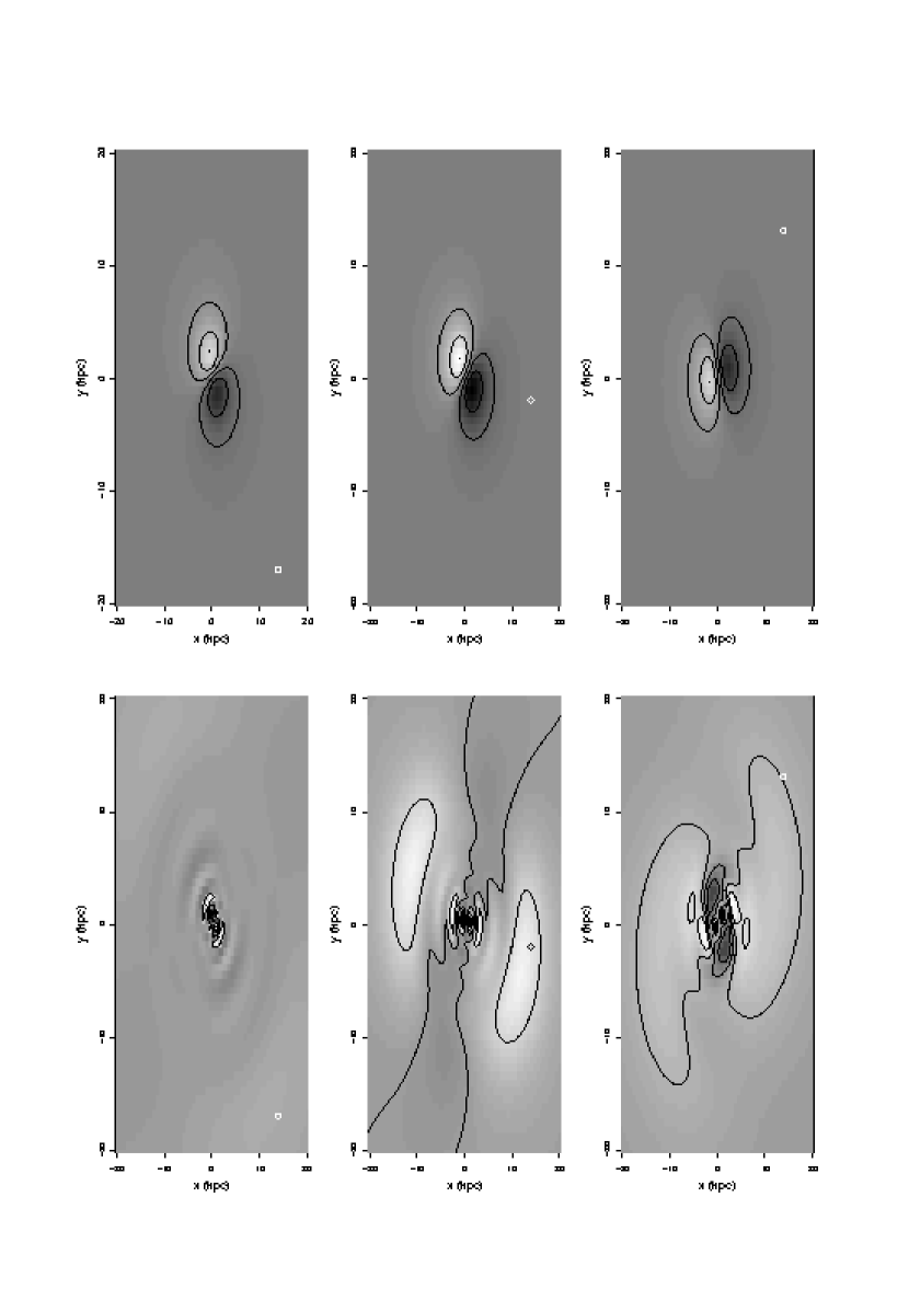
Figure 16.— Density distortion of the primary galaxy at three phases of the fly-by with $V=200$ km/s and $p/R_{h}=1.0$. Upper panels show the dipole response; lower panels show the quadrupole response. The white dot shows the position of the perturber.

Figure 17.— Perturbation energy as a function of the orthogonal function indices for three phases shown in Figure 16. In each panel, open circles (crosses) indicate dipole (quadrupole) response. Each curve is normalized to the maximum value of $E_{p}(n)$.

Figure 17 shows plots of $E_{p}(n)$ for the same case and phases shown in Figure 16 describing the distribution of energy at different scales. Similar to the results in §3, the dipole response is dominated by large scale features while in the quadrupole response there is a non negligible contribution to the total energy of the perturbation from features at smaller scales.

4.2. Diagnostics of asymmetry in the primary galaxy

We employ an established asymmetry diagnostic to compare our predictions to observations and suggest a straightforward generalization which will help discriminate the response mechanism considered here from others. We will focus our attention on an asymmetry parameter $A$ for image data, defined as

$$A\equiv{1\over 2}{\sum|I(x,y)-I_{rot}(x,y)|\over\sum I(x,y)}$$ (7)

where $I(x,y)$ and $I_{rot}(x,y)$ are the brightness at a given point $(x,y)$ of the original image and in the image after a 180 degree rotation about the position of the maximum density of the primary system, respectively.

For our calculation we use the density of the system on the orbital plane and thus our theoretical values are not affected by any projection effect and will provide a measure of the real asymmetry of the plane. Observational values, on the other hand, are determined using the projected density and part of the underlying asymmetry of the orbital plane is likely to be washed out. In order to evaluate the effect of using the projected density on the orbital plane instead of the real plane density, we have repeated some of the calculations: we have found that, for a given value of $m/M$, the values of $A$ obtained using the projected density are smaller than those obtained using the real plane density by a constant factor independent of the perturber orbital parameters and approximately equal to 3.8; this implies that, using the projected density, all the values of $A$ (as well as those of the parameter $S$ introduced later in this section) and the numerical parameters in the scaling laws of the amplitude of $A$ with the perturber’s orbital parameters discussed in this section are not altered but they are produced by a perturber with a mass equal to $0.38M$ (instead of $0.1M$ adopted in the rest of this section).

The $A$ parameter was first introduced by Abraham et al. (1996a) to estimate the asymmetry observed in galaxies in the Medium Deep Survey and in the Hubble Deep Field and it has been recently adopted in several investigations on the morphology of galaxies in different environments (e.g. van den Bergh et al. 1996, Naim, Ratnatunga & Griffiths 1997, Marleau & Simard 1998, Conselice & Bershady 1998, Conselice & Gallagher 1999). The values of $A$ reported in these investigations range from $0$ for the most symmetric systems to $0.5$ for those showing the strongest asymmetries. A comparison of the distribution of values of $A$ for a sample of local galaxies, galaxies in the Medium Deep Survey and in the Hubble Deep Field was reported by Abraham et al. (1996a, 1996b). Their results show that the distribution of $A$ for galaxies in the HDF is significantly skewed toward larger values of $A$ compared to the distribution for galaxies in the MDS which in turn is skewed to larger values of $A$ relative to the distribution of $A$ for a sample of local galaxies. This trend is likely to be due to the higher interaction and merging rates for distant galaxies in the HDF and the MDS. In principle, a high value of $A$ could also result from an asymmetric distribution of star forming regions, however a recent investigation by Conselice & Bershady (1998) shows that the colors of many asymmetric objects in the HDF are not blue enough to support this hypothesis.

In addition, we have calculated the displacement, $S$, between the position of the peak of the density of the primary system and the position of its center of mass. The estimate of $S$ is of particular interest since many observations have provided evidence of off-center galactic nuclei and of significant displacement of isophotal centers (see e.g. Miller & Smith 1992 for a short overview of several observational analyses). In particular, Naim et al. (1997) have adopted distances between the centers of different isophotal curves as one of the diagnostic parameters characterizing the degree of peculiarity of galaxies in a sample of moderate-redshift systems and Mendes de Oliveira & Hickson (1994) have investigated the morphology of early-type galaxies in compact groups and used the evidence of non-concentric isophotes as a diagnostic to identify perturbed galaxies.

4.3. Evolution of the asymmetry diagnostic parameters

Figure 18 shows the time evolution of the asymmetry parameter $A$ defined above (eq. 7).

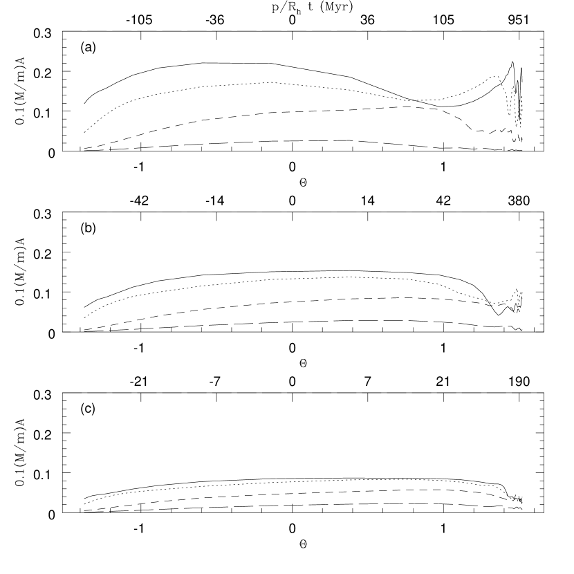
Figure 18.— Evolution of the asymmetry parameter $A$ (see eq.7) as a function of the position angle for the fly-bys with $V=200$ km/s (a), $V=500$ km/s (b) and $V=1000$ km/s (c). In each panel the four curves correspond to different values of the pericenter of perturber: $p/R_{h}=0.5$ (solid line), $p/R_{h}=1.0$ (dotted line), $p/R_{h}=3.0$ (dashed line), $p/R_{h}=7.0$ (long dashed line).

Although several well-documented processes contribute to the observed distorted morphologies, the majority of the values in the distribution of $A$ obtained for galaxies in the MDS and in the HDF by Abraham et al. (1996) (see their Fig. 2) fall well in the range of values of $A$ we have obtained in our analysis. Mergers and strong interactions with more massive systems are likely to be responsible for the production of the extreme values of $A$ ($A\hbox{ \hbox to0.0pt{\raise 1.82986pt\hbox{$>$}\hss}\lower 2.79857pt\hbox{$\sim$} }0.3$) observed in some galaxies. We point out that the observational data refer to all the morphological types including spiral galaxies to which our results do not directly apply.

Figure 19 shows the time evolution of $S$.

Table 5
Best fit parameters for the scaling of
$\max(0.1M/m)A$ and $\max(0.1M/m)S~{}(pc)$
with the relative velocity of encounters
id.	$K_{A}$	$\alpha_{A}$	$K_{S}$	$\alpha_{S}$
$p/R_{h}=0.5$	0.24	0.6	$2.5\times 10^{3}$	0.6
$p/R_{h}=1.0$	0.19	0.5	$1.9\times 10^{3}$	0.5
$p/R_{h}=3.0$	0.11	0.4	$0.8\times 10^{3}$	0.4
$p/R_{h}=7.0$	0.03	0.1	$0.1\times 10^{3}$	0.0
The scaling of $\max(0.1M/m)^{2}A$ and $\max(0.1M/m)^{2}S$ with
the relative velocity of encounters, $V$, has been fitted using
the function $f(V)={K\over(V(\hbox{km/s})/200)^{\alpha}}$.

As expected, the trend with $V$ and $p$ is similar to that obtained for the asymmetry parameter $A$, with slow and close encounters being those capable of producing the largest values of $S$. Even fly-bys with large values of $p$ are capable of affecting the inner regions of the primary galaxies and lead to a significant displacement of the position of the density peak from the center of mass of the system.

Figure 19.— Evolution of the distance, $S$, between the position of the density peak and its center of mass as a function of the position angle of the perturber for the fly-bys with $V=200$ km/s (a), $V=500$ km/s (b) and $V=1000$ km/s (c). In each panel the four curves correspond to different values of the pericenter of perturber: $p/R_{h}=0.5$ (solid line), $p/R_{h}=1.0$ (dotted line), $p/R_{h}=3.0$ (dashed line), $p/R_{h}=7.0$ (long dashed line).

The dependence of both asymmetry parameters on $V$ and $p$ is summarized in Figure 20 which shows the maximum values taken by $A$ and $S$ as a function of $p/R_{h}$ for the three values of $V$ considered.

Figure 20.— Maximum value taken by $A$ (panel a), $S$ (panel b) as a function of the perturber pericenter of the orbit of the perturber. The three curves in each panel corresponds (from the upper to the lower curve) to $V=200$ km/s, $V=500$ km/s and $1000$ km/s.

We have fit the scaling of $\max 0.1(M/m)A$ and $\max 0.1(M/m)S$ with the relative velocity of the encounter for different values of $p$ with a power-law $K/(V(\hbox{ km s}^{-1})/200)^{\alpha}$ and we report the values obtained for the cases investigated in Table 5. These fits are not valid in the limit of adiabatic encounters where the strength of the perturbation and of the diagnostic parameters tend to a constant value as described previously (see §3.1).

4.4. Radial dependence of the asymmetry parameter $A$

Fly-by interactions described here produce structure on well defined scales (cf. Fig. 16), however, the sum in equation (7) washes out the signature of our predicted response by averaging over regions with little distortion. To improve sensitivity, we propose an incomplete form of the asymmetry parameter $A(r)$ which restricts the sum in equation (7) to pixels enclosed by a circle of radius $r$ from the position of the peak of density $R_{p}$.

Figure 21.— Plot of the asymmetry parameter, $A$, as a function of time and radius of the area (centered at the position of the peak of density) considered for its calculation for the fly-by with $V=500$ km/s and $p/R_{h}=0.5$.

Figure 22.— (a) Radial profile of $A$ (normalized to its maximum value) for fly-bys with $p/R_{h}=1.0$ and $V=200$ km/s (solid line), $V=500$ km/s (dotted line), $V=1000$ km/s (dashed line); each curve correspond to the radial profile of $A$ when the total $A$ is maximum. (b) Same as (a) but for fly-by with $V=500$ km/s and $p/R_{h}=0.5$ (solid line), $p/R_{h}=1.0$ (dotted line), $p/R_{h}=3.0$ (dashed line), $p/R_{h}=7.0$ (long dashed line).

Figure 21 shows the plot of $A(t,r)$ (calculated for $m/M=0.1$) for the case with $V=500$ km/s and $p/R_{h}=0.5$. The appearance of $A(t,r)$ is qualitatively similar for the other cases investigated. The profile of $A$ at any given time has a maximum at $0.3\hbox{ \hbox to0.0pt{\raise 1.82986pt\hbox{$<$}\hss}\lower 2.79857pt\hbox{$\sim$} }r/R_{h}\hbox{ \hbox to0.0pt{\raise 1.82986pt\hbox{$<$}\hss}\lower 2.79857pt\hbox{$\sim$} }1.0$ with a subsequent decrease which is steeper near the absolute maximum of $A(t,r)$ and shallower far from this maximum. The value of $A$ always tends to a constant for large values of $r$. In Figure 22a we compare the radial profile of $A$ for the three fly-bys with $p/R_{h}=1.0$ and $V=200,~{}500,~{}1000~{}$ km/s. The three curves show the run of $A(r)$ at peak and each curve is normalized to the maximum value of $A(r)$, $A_{max}$. The radial location of $A_{max}$ and the shape of $A(r)$ do not depend significantly on the velocity of the perturber in these half-mass units. Figure 22b compares $A(r)/A_{max}$ for all the fly-bys with $V=500$ km/s and with the different values of $p/R_{h}$ investigated. The location of the peak of $A(r)/A_{max}$ depends very slightly on $p/R_{h}$ while there is a marked difference between the slope of $A(r)/A_{max}$ after the peak for the fly-bys with small pericenters ($p/R_{h}<1.0$) and those with larger values of $p/R_{h}$ $(p/R_{h}>3.0)$. A distinct peak in the radial profile of $A$ is present only at some phases of the encounter and this could be difficult to capture in observations. On the other hand the decrease at small values of $r$ is a feature common to all the phases of the orbit of the perturber and it should be an observable signature.

4.5. Summary and discussion

In this section, we have studied the response of a high-concentration spherical stellar system to the perturbation induced by a fly-by. We represent the outer profiles of cluster ellipticals by a high-concentration King model; we choose a King profile rather than a core-free model for numerical convenience. A deformation in the structure of the primary galaxy is directly observable and we explored quantitative measures of the asymmetry produced during the fly-by encounter. In the end, we focussed our attention on the asymmetry parameter $A$, introduced by Abraham et al. (1996a, 1996b) and measured for a number of local galaxies and in galaxies in the MDS and in the HDF fields, and on the shift $S$, between the position of the peak of the density of the system and its center of mass. We present the time evolution, the scaling with the perturber orbit and the radial dependence of the asymmetry to facilitate estimates for a wide variety of environments.

The values of $A$ caused by fly-bys range from $A\approx 0$ to $A\approx 0.2$ and this same range of values of $A$ is found in observations of numerous local galaxies and distant galaxies in the MDS and in the HDF fields (Abraham et al. 1996a, 1996b). Extreme values of $A$ observed for some galaxies in the HDF field ($A\hbox{ \hbox to0.0pt{\raise 1.82986pt\hbox{$>$}\hss}\lower 2.79857pt\hbox{$\sim$} }0.2$) are probably caused by mergers. The quantities $A$ and $S$ reach their maximum values when the perturber is close to the pericenter of its orbit. As evident in Figure 18, the distortions may be long-lived; in some cases the perturber can be quite distant from the primary system and therefore we can expect some non-negligible values of $A$ and $S$ even without any close companion in the vicinity of the primary.

Our results show that the values of $A$ and $S$ will be determined by both the distribution of relative encounter velocities and the density of the environment. In short, richer groups and clusters with lower velocity dispersions will lead to high values of $A$ and $S$. Figure 18 shows that disturbances persist until $\Theta\hbox{ \hbox to0.0pt{\raise 1.82986pt\hbox{$>$}\hss}\lower 2.79857pt\hbox{$\sim$} }1.4$ or roughly $\tau\sim 5\times 10^{8}$ years after the pericenter passage. In order to provide a quantitative indication of the dependence of the response on the environmental conditions, we have calculated the probability that a galaxy has an encounter in the time interval $\tau$ such that $\max A\geq 0.1$ assuming that the perturber has a mass $m=0.1M$ (or $m=0.38M$ if the projected density is used for the calculation of $A$). For our fiducial system $\tau=5\times 10^{8}$ yrs and $m=10^{11}M_{\odot}$, the probability $P$ of having such an encounter is given by

$$P=n\pi p^{2}(V)V\tau$$ (8)

where $n$ is the galaxy number density of the environment and $p(V)$ is the pericenter distance for which $\max A=0.1$ during an encounter with velocity $V$. The function $p(V)$ has been determined using the parametrization reported in Table 5 for the values of $V$ available from our numerical investigation and then fitting these points with a function of the form $K/V^{\beta}$. We obtain

$$P(n,V)={10^{-3}n(\hbox{Mpc}^{-3})\over(V(\hbox{km s}^{-1})/200)^{1.44}}$$ (9)

and describe this function in Figure 23. This quantifies our finding that galaxies in environments characterized by high density and low-velocity dispersion, like compact groups, will be more likely to show signs of past or recent interactions in agreement with the results of a number of investigations (see e.g. Zepf & Whitmore 1993, Mendes de Oliveira & Hickson 1994). These observational studies argue that the fraction of distorted morphologies in compact groups is larger than the fraction observed in clusters (which have similar number densities but higher velocity dispersions) and in sample of field galaxies (which are likely to suffer low-velocity encounters but in a low-density environment). Assuming that young galaxies were located in dense environments and characterized by lower, previrialized velocity dispersions, our conclusions are consistent with the results of Abraham et al. (1996b) who have shown that the distribution of $A$ for galaxies in the HDF is skewed toward high values compared to that for galaxies in the MDS which, in turn, are more asymmetric than local field galaxies.

Figure 23.— Loci of constant probability $P(n,V)$ for an encounter in the past $t=10t_{dyn}$ such that $\max A\geq 0.1$. The vertical and horizontal axes describe the number density of the environment and relative velocity of encounters.

An additional useful diagnostic is the ratio of the perturber to the primary masses necessary to produce a given value of $\max A$. This is easily obtained from the fits discussed in §4.3 and is given by

$$\left({m\over M}\right)_{\max A}={0.1\over K_{A}}\max A\left({V(\hbox{km/s})\over 200}\right)^{\alpha_{A}},$$ (10)

where the values of $K_{A}$ and $\alpha_{A}$ depend on $p/R_{h}$ (cf. Table 5). The four frames in Figure 24 show the contour plots of $(m/M)_{\max A}$ in the plane $\max A-V$ (as we discussed at the beginning of this section, if the projected density is used for the calculation of $A$ the values of $m/M$ are larger than those reported in Fig. 24 by a factor 3.8). Any environment producing low-velocity, close encounters can lead to significant asymmetries ($\max A\hbox{ \hbox to0.0pt{\raise 1.82986pt\hbox{$>$}\hss}\lower 2.79857pt\hbox{$\sim$} }0.1$) in the primary system even by low-mass perturbers ($m/M\simeq 0.02-0.1$). For example, consider a system with a mass and a radius equal to those of our fiducial system ($M=10^{12}~{}M_{\odot}$, $R=120$ kpc). An encounter with a perturber with $m/M=0.05$ with relative velocity $V=200$ km/s leads to $\max A=0.1$ if $p/R_{h}=1.0$ ($p\simeq 14$ kpc for our fiducial system). Low-mass interlopers with pericenters close to the primary center could lead to significant asymmetries in cluster ellipticals as well.

Figure 24.— Loci of constant relative perturber mass necessary to have a maximum value of the asymmetry parameter equal to $\max A$ during an encounter with relative velocity $V$. Pericenter distances label each frame.

Fly-by encounters yield the following signature in our radially-dependent asymmetry parameter, $A(r)$: 1) a decrease at small radii, 2) a peak around $0.3\hbox{ \hbox to0.0pt{\raise 1.82986pt\hbox{$<$}\hss}\lower 2.79857pt\hbox{$\sim$} }r/R_{h}\hbox{ \hbox to0.0pt{\raise 1.82986pt\hbox{$<$}\hss}\lower 2.79857pt\hbox{$\sim$} }1.0$ and 3) a convergence to a constant value at large radii. Although we have not predicted the signature of $A(r)$ for scenarios other than fly-bys, we believe an observational investigation would provide a test of the mechanism proposed here and would be a general probe of asymmetric structure. The computation of $A(r)$ is relatively straightforward with the data already available.

5. Conclusions

We have explored the structure and the persistence of the features in dark halos and cluster ellipticals excited by an unbound (or fly-by) interaction over a range of different galactic environments. The main conclusions of our analysis are as follows:

1. Fly-by encounters which penetrate the outer regions of a galaxy can lead to asymmetric features well inside the half-mass radius. The distortion of a dark halo may affect its disk (e.g. Weinberg 1998b).

2. In dark halos the lowest-order damped modes yield strong features which persist well after the perturber’s passage and could account for distorted morphologies in galaxies without obvious close companions. Such damped modes are a natural part of the collisionless response but are difficult to resolve in N-body simulations with modest particle number ($N\hbox{ \hbox to0.0pt{\raise 1.82986pt\hbox{$<$}\hss}\lower 2.79857pt\hbox{$\sim$} }10^{6}$) due to noise.

3. The strength of the response depends both on the velocity of the perturber and on the pericenter of its orbit; low-velocity, close encounters produce the strongest perturbations.

4. Completely external fly-by encounters will produce a strong response if the perturber is more massive than the primary. For example such encounters can produce significant effects on spiral galaxies in clusters where they are likely to interact with more massive giant ellipticals and on dwarfs in the vicinity of normal galaxies.

5. A proposed generalization of the asymmetry parameter $A$ (Abraham et al. 1996a), provides a diagnostic of the radial structure of the asymmetry and a test of the mechanism explored here in particular. Our predicted range of $A$ is similar to that observed for the majority of galaxies in the Medium Deep Survey, in the Hubble Deep Field and for local galaxies. We quantify the range of high-density, low-velocity dispersion environments expected to produce significant distortions by fly-by encounters. Indeed, compact groups have been shown to have a significant fraction of distorted galaxies.

Additional discussion is provided in §3.4 for dark halos and in §4.5 for cluster ellipticals.

Future work will explore the properties of the response for cuspy galaxies; the magnitude of the resonant coupling to the inner galaxy in core-free profiles would nicely complement the present work. We plan to further investigate the effects of the halo distortions on an embedded stellar and gaseous disk, by extending our current study to explore the response of the disk and to quantify the induced deformations. This will permit direct comparisons with the observed distortions in the morphology of disks as well as to study possible effects of these distortions on their kinematics. In particular, the effects of even small deformations in the morphologies of disks could significantly affect their kinematics possibly giving rise to the observed scatter in the Tully-Fisher relation as suggested by Franx & de Zeeuw (1992).

References

Abraham R.G.,van den Bergh S., Glazebrook K., Ellis R.S., Santiago B.X., Surma P., & Griffiths R.E. 1996a, ApJS, 107,1
Abraham R.G., Tanvir N.R., Santiago B.X., Ellis R.S., Glazebrook K., & van den Bergh S. 1996b, MNRAS, 279, L47
Barnes, J. 1998, in Galaxies : Interactions and Induced Star Formation : Saas-Fee Advanced Course 26 Lecture Notes 1996 Swiss Society for Astrophysics and Astronomy)
Barnes, J., & Hernquist, L. 1992, ARA&A, 30, 705
Bertin, G., & Mark, J.W.K., 1980, A&A, 1980, 88, 289
Bertin G., & Pegoraro F., 1989, In ESA, Proceedings of International School and Workshop on Plasma Astrophysics, Volume 1 p.329
Bertin G., Pegoraro F., Rubini F., & Vesperini, E. 1994, ApJ, 434, 94
Brinchmann J. et al. 1998, ApJ, 499, 112
Butcher H, & Oemler, A. 1978, ApJ, 219, 18
Butcher H, & Oemler, A. 1984, ApJ, 285, 426
Couch W.J., Barger A.J. Smail I., Ellis R.S., & Sharples R.M. 1998, ApJ, 497, 188
Conselice C.J., & Gallagher III, J.S. 1999, AJ, 117, 75
Conselice C.J., & Bershady M. 1998, preprint, astro-ph 9812299
Dressler A. 1980, ApJ, 236, 351
Dressler A., Oemler A., Butcher H., & Gunn J.E. 1994a, ApJ, 430, 107
Dressler A., Oemler A., Sparks W.B., & Lucas R.A. 1994b, ApJ, 435, L23
Dressler et al. 1997, ApJ, 490, 577
Edmonds A.R. 1960, Angular Momentum in Quantum Mechanics, Princeton University Press, Princeton, New Jersey
Franx M., & de Zeeuw T. 1992, ApJ, 392, L47
Haynes M.P., Hogg D.E., Maddalena R.J., Roberts M.S., & van Zee L. 1998, AJ, 115, 62
Hubble E., & Humason M.L. 1931, ApJ, 74, 43
Kalnajs A.J. 1977, AJ, 212, 637
Kochanek C.S. 1996, ApJ, 457, 228
Kornreich D.A., Haynes M.P, & Lovelace R.V. 1998, AJ, 116, 2154
Levine S.E., & Sparke L.S. 1998, ApJ, 496, L13
Marleau F.R., & Simard L. 1998, ApJ, 507, 585
Mendes de Oliveira C., & Hickson P. 1994, ApJ, 427, 684
Miller R.H., & Smith B.F. 1992, ApJ, 393, 508
Moore B., Katz N., Lake G., Dressler A., Oemler A., 1996, Nature, 379, 613
Moore B., Lake G., & Katz N. 1998, ApJ, 495, 139
Murali, C. 1998, preprint, astro-ph 9811223
Murali, C., & Tremaine S. 1998, MNRAS, 296, 749
Naim A., Ratnatunga U., & Griffiths R.E., ApJ, 476, 510
Nelson, R.W., & Tremaine S., 1995, MNRAS, 275, 897
Nelson, R.W., & Tremaine S., 1996, in Lahav O.,Terlevich E., Terlevich R., eds, Proceedings of the 36th Herstmonceux Conference, Gravitational Dynamics, Cambridge Univ. Press, Cambridge, p.73
Oemler A. 1974, ApJ, 194, 1
Palmer P.L., & Papaloizou J. 1987, MNRAS, 224, 1043
Palmer P.L. 1994, Stability of Collisionless stellar systems, Kluwer Academic Publishers, Dordrecht
Polyachenko V.L., & Shukhman I. 1981, Sov. Astron., 25,533
Reshetnikov V., & Combes F. 1998, A&A, 337, 9
Reshetnikov V., & Combes F. 1999, preprint, astro-ph9906063
Richter O., & Sancisi R. 1994, A&A, 290, L9
Rubin V., Waterman A.H., & Kenney J.D.P., preprint, astro-ph 9904050
Rudnick G., & Rix H.W. 1998, AJ, 116, 1163
Saha P. 1991, MNRAS, 248, 494
Sellwood J., & Merritt D. 1994, ApJ, 425, 530
Swaters R.A., Schoenmakers R.H.M., Sancisi R., & van Albada T.S. 1998, preprint, astro-ph 9811424
Tremaine S., & Weinberg M.D. 1984, MNRAS, 209, 729
van den Bergh S., Abraham R.G., Ellis R.S., Tanvir N.R., Santiago B.X., & Glazebrook K. 1996, AJ, 112, 359
Weinberg, M.D. 1989, MNRAS, 239, 549
Weinberg, M.D. 1994, ApJ, 421, 481
Weinberg, M.D. 1995, ApJ, 455, L31
Weinberg, M.D. 1998a, MNRAS, 297, 101
Weinberg, M.D. 1998b, MNRAS, 299, 499
Weinberg, M.D. 1999, AJ, 117, 629
Zaritsky D., & White S.D.M. 1994, 435, 599
Zaritsky D., & Rix H.W. 1997, ApJ, 477, 118
Zaritsky D., Smith R., Frenk C., & White S.D.M. 1997, 478, 39
Zepf S.E., & Whitmore B.C. 1993, ApJ, 418,72

Appendix A Details of the derivation of the matrix equation

Our results are based on an explicit solution for the response of a spherical stellar system to the perturbation induced by a perturber with mass $m$ on rectilinear trajectory with pericenter $p$. Specifically, we solve the coupled linearized collisionless Boltzmann equation for the distribution function of the primary stellar system and Poisson’s equation (cf. §2)

$${\partial f_{1}\over\partial t}+{\partial f_{1}\over\partial{\bf w}}{\partial H_{0}\over\partial{\bf I}}-{\partial f_{0}\over\partial{\bf I}}{\partial H_{1}\over\partial{\bf w}}=0,$$

$$\nabla^{2}\Phi_{1}=4\pi G\rho_{1},$$

where the subscript $0$ denotes the equilibrium quantities and the subscript $1$ denotes the first order perturbation of the distribution function $f$, and Hamiltonian $H$. The perturbed potential, $\Phi_{1}$, is the sum of the tidal potential due to the perturber, $\Phi_{p}$, and the gravitational potential of the response to the perturbation, $\Phi_{resp}$. After performing the Laplace transform in time, the Fourier transform in the angle variables and solving for $f_{1}$, equation (1) becomes

$$\tilde{f}_{{{\mbox{\boldmath$\gamma$}}}1}=i{{\mbox{\boldmath$\gamma$}}}{\partial f_{0}\over\partial{\bf I}}{\tilde{\Phi}_{p,{{\mbox{\boldmath$\gamma$}}}}+\tilde{\Phi}_{resp,{{\mbox{\boldmath$\gamma$}}}}\over s+i{{\mbox{\boldmath$\gamma$}}}\cdot{{\mbox{\boldmath$\omega$}}}},$$ (A1)

where we denote the Laplace transform of a quantity $y(t)$ by $\tilde{y}(s)$ and the Fourier transform of a quantity $y({\bf w})$ by $y_{{\mbox{\boldmath$\gamma$}}}$ with ${{\mbox{\boldmath$\gamma$}}}=(\gamma_{1},\gamma_{2},\gamma_{3})$ indicating the vector of integer indices for the discrete Fourier expansion in the angle variables. The frequencies associated to the angle variables are denoted by ${{\mbox{\boldmath$\omega$}}}=\partial H_{0}/\partial{\bf I}$.

Following the approach adopted in Weinberg (1989), we will use a potential-density biorthogonal basis, $u^{l}_{i},~{}d^{l}_{i}$ to expand the perturbed quantities $\Phi_{1}$ and $\rho_{1}$. The pairs $u_{i}^{l}$, $d_{i}^{l}$ are solutions of the Poisson equation. The basis we have adopted is obtained by numerical solution of the associated Sturm-Liouville problem in which the lowest order basis functions are tailored to the background equilibrium model following Weinberg (1999). The solution to the coupled equation, which determines the response of the halo to the perturbation, then reduces to the solution of an algebraic integral equation for the coefficients of the expansion. The subsections below sketch the main steps in the derivation of the algebraic equation for the coefficients of the expansion from equation (A1) (see e.g. Weinberg 1989 for additional details).

A.1. Expansion of the perturbation potential in action-angle variables

We begin by expanding the perturbing potential, $\Phi_{p}$, in terms of spherical harmonics $Y_{lm}(\theta,\phi)$ (where $\theta$ and $\phi$ denotes the angular coordinates inside the primary stellar system). Up to quadrupole order, the potential of a point mass perturber can be written as

$$\Phi_{p}=Gm\left[\sqrt{{2\pi\over 3}}\left(-e^{-i\Theta}Y_{1,1}+e^{i\Theta}Y_{1,-1}\right){r_{<}\over r_{>}^{2}}+\sqrt{{\pi\over 5}}\left(-Y_{2,0}+\sqrt{{3\over 2}}e^{-2i\Theta}Y_{2,2}+\sqrt{{3\over 2}}e^{2i\Theta}Y_{2,-2}\right){r_{<}^{2}\over r_{>}^{3}}\right]$$ (A2)

where $\Theta(t)=\arctan({Vt/p})$ is the position angle of the perturber defined as the angle between the axis from the center of the system to the pericentric position of the perturber and the axis from the center to the position at time $t$. We define the usual quantities $r_{<}=\min(r,R)$, $r_{>}=\max(r,R)$ where $r$ and $R$ are the radial coordinate inside the stellar system and the distance between the center of the system and the perturber, respectively.

Following Tremaine & Weinberg (1984), the radial part of the perturbing potential is expanded in terms of the basis function $u^{l}_{i}$ and each resulting term is expressed in the form $u^{l}_{i}(r)Y_{lm}(\theta,\phi)$ as a Fourier series in the angle variables ${\bf w}$. We finally obtain:

$$\Phi_{p} = Gm\sum_{{\mbox{\boldmath$\gamma$}}=-\infty}^{\infty}\delta_{\gamma_{3}m}\left[\sqrt{{\pi\over 5}}\left(-V_{2\gamma_{2}\gamma_{3}}\delta_{\gamma_{3}0}+\sqrt{3\over 2}e^{-2i\Theta}V_{2\gamma_{2}\gamma_{3}}\delta_{\gamma_{3}2}+\sqrt{3\over 2}e^{2i\Theta}V_{2\gamma_{2}\gamma_{3}}\delta_{\gamma_{3}-2}\right)X_{2\gamma_{2}\gamma_{3}}^{\gamma_{1}}+\right.$$ (A3)

$$\left.\sqrt{\left({2\pi\over 3}\right)}\left(-e^{-i\Theta}V_{1\gamma_{2}\gamma_{3}}\delta_{\gamma_{3}1}+e^{i\Theta}V_{1\gamma_{2}\gamma_{3}}\delta_{\gamma_{3}-1}\right)X_{1\gamma_{2}\gamma_{3}}^{\gamma_{1}}\right]e^{i{\mbox{\boldmath$\gamma$}}{\bf w}}$$

where

$$X_{l\gamma_{2}\gamma_{3}}^{\gamma_{1}}={1\over 2\pi}\int_{-\pi}^{\pi}dw_{1}u_{\gamma_{3}}^{l}(r)e^{-i[\gamma_{1}w_{1}+\gamma_{2}(w_{2}-\psi)]}$$ (A4)

and

$$V_{l\gamma_{2}\gamma_{3}}(\beta)=r^{l}_{\gamma_{2}\gamma_{3}}(\beta)Y_{l\gamma_{3}}(\pi/2,0)i^{\gamma_{3}-\gamma_{2}}.$$ (A5)

The angle $\beta$ is the inclination of the orbital plane to the equatorial plane and $r^{l}_{\gamma_{2}\gamma_{3}}(\beta)$ are the components of the rotation matrices (see e.g. Edmonds 1960).

A.2. Derivation of matrix equation

Similarly, we can express the perturbing and the response potential in the form

$$\Phi=\sum_{l,{{\mbox{\boldmath$\gamma$}}}}V_{l\gamma_{2}\gamma_{3}}(\beta)\sum_{j}a^{j}_{l\gamma_{3}}(t)X_{l\gamma_{2}\gamma_{3}}^{\gamma_{1},j}e^{i{{\mbox{\boldmath$\gamma$}}\cdot\bf w}}.$$ (A6)

For the perturbing potential, each coefficient $a^{j}_{l\gamma_{3}}(t)$ can be expressed as the product of a time-independent coefficient, $b^{j}_{l\gamma_{3}}$, and a function of time depending only on $l$ and $\gamma_{3}$, $g_{l\gamma_{3}}(t)$. The functional form of $g_{l\gamma_{3}}(t)$ can be easily derived for any value of $l$ and $\gamma_{3}$ using equation (A2). For example, for $r<R$, $l=2$ and $\gamma_{3}=2$, one finds $g_{22}=\cos^{3}\Theta(t)e^{-2i\Theta(t)}.$ Equation (A1) now takes the form

$$\tilde{f}_{{\mbox{\boldmath$\gamma$}}1}={i{\mbox{\boldmath$\gamma$}}\cdot{\partial f_{0}\over\partial{\bf I}}\over s+i{\mbox{\boldmath$\gamma$}}\cdot{{\mbox{\boldmath$\omega$}}}}\left[\sum_{l}V_{l\gamma_{2}\gamma_{3}}(\beta)\sum_{j}\tilde{a}^{j}_{l\gamma_{3}}(s)X_{l\gamma_{2}\gamma_{3}}^{\gamma_{1},j}e^{i{{\mbox{\boldmath$\gamma$}}\cdot\bf w}}+\sum_{l}V_{l\gamma_{2}\gamma_{3}}(\beta)\sum_{j}b^{j}_{l\gamma_{3}}\tilde{g}_{l\gamma_{3}}(s)X_{l\gamma_{2}\gamma_{3}}^{\gamma_{1},j}e^{i{{\mbox{\boldmath$\gamma$}}\cdot\bf w}}\right].$$ (A7)

For self-consistency, the response density, which is obtained by integrating equation (A7) over the velocity coordinates, $\rho_{1}^{resp}$, must be equal to the density $\rho_{1}^{P}$ determined by the Poisson’s equation with $\Phi_{1}=\Phi_{1}^{resp}$. Imposing the condition

$$\tilde{\rho_{1}}^{P}=\tilde{\rho_{1}}^{resp},$$ (A8)

multiplying both sides of equation(A8) by $Y_{l\gamma_{3}}^{*}u^{l}_{i}$ and integrating over the spatial coordinates, we obtain the following equation for the coefficients

$$\tilde{a}^{i}_{l\gamma_{3}}(s)=\sum_{j}M^{ij}_{l\gamma_{3}}(s)[\tilde{a}^{j}_{l\gamma_{3}}(s)+b^{j}_{l\gamma_{3}}\tilde{g}(s)].$$ (A9)

Equivalently, this may be written as a matrix equation:

$${\bf\tilde{a}}_{l\gamma_{3}}(s)={\bf D}_{l\gamma_{3}}^{-1}(s){\bf M}_{l\gamma_{3}}(s)[{\bf b}_{l\gamma_{3}}\tilde{g}(s)]$$ (A10)

where the elements of the matrix ${\bf M}_{l\gamma_{3}}(s)$ are defined as

$$M^{ij}_{l\gamma_{3}}(s)\equiv\sum_{\gamma_{1},\gamma_{2}}\int\hbox{d}{\bf I}\hbox{d}{\bf w}{i{\mbox{\boldmath$\gamma$}}\cdot{\partial f_{0}\over\partial{\bf I}}\over s+i{\mbox{\boldmath$\gamma$}}\cdot{{\mbox{\boldmath$\omega$}}}}V^{*}_{l-\gamma_{2}-\gamma_{3}}V_{l\gamma_{2}\gamma_{3}}X_{l-\gamma_{2}-\gamma_{3}}^{\gamma_{1},i*}X_{l\gamma_{2}\gamma_{3}}^{\gamma_{1},j}$$ (A11)

and

$${\bf D}_{l\gamma_{3}}\equiv{\bf I}-{\bf M}_{l\gamma_{3}}.$$ (A12)

Equations (A9) or (A10) completely determines the response to the perturbation induced by the perturber. For ${\bf b}=0$ (no external perturbation), one obtains the following nonlinear eigenvalue problem

$$\tilde{a}^{i}_{l\gamma_{3}}(s)=\sum_{j}M^{ij}_{l\gamma_{3}}(s)[\tilde{a}^{j}_{l\gamma_{3}}(s)].$$ (A13)

The eigenvalues of this problem are the frequencies of the point modes of the stellar system: frequencies with $Re(s)>0$ correspond to unstable growing modes while for stable damped modes $Re(s)<0$.

A.3. Inverse Laplace transform

Solution of equation (A9) describes the evolution in frequency space. In order to get the time evolution of the perturbation we need to perform the inverse Laplace transform of equation (A9). This yields the following expression for the coefficients ${\bf a}_{l\gamma_{3}}(t)$

$${\bf a}^{i}_{l\gamma_{3}}(t)=\left[\sum_{\gamma_{1},\gamma_{2}}\int\hbox{d}{\bf I}\hbox{d}{\bf w}D^{-1}_{ik}(-i{{\mbox{\boldmath$\gamma$}}}\cdot{{\mbox{\boldmath$\omega$}}})\mu^{kj}e^{-i{{\mbox{\boldmath$\gamma$}}}\cdot{{\mbox{\boldmath$\omega$}}}t}\int_{-\infty}^{t}g_{l\gamma_{3}}(t^{{}^{\prime}})e^{i{{\mbox{\boldmath$\gamma$}}}\cdot{{\mbox{\boldmath$\omega$}}}t^{{}^{\prime}}}\hbox{d}t^{{}^{\prime}}\right]b^{j}_{l\gamma_{3}},$$ (A14)

where, to simplify the notation, we have defined

$$\mu^{kj}\equiv{i{\mbox{\boldmath$\gamma$}}\cdot{\partial f_{0}\over\partial\bf{I}}}V^{*}_{l-\gamma_{2}-\gamma_{3}}V_{l\gamma_{2}\gamma_{3}}X_{l-\gamma_{2}-\gamma_{3}}^{\gamma_{1},i*}X_{l\gamma_{2}\gamma_{3}}^{\gamma_{1},j}.$$ (A15)

Equation (A14) does not take into account the zeros of det ${\bf D}(s)$ which are the point modes of the primary system. Since we will consider only systems known to be stable, there are no modes with $Re(s)>0$, while modes with $Re(s)<0$ will be damped and die away with time. Nevertheless, as shown in Weinberg (1994), for King models some modes can be very weakly damped and persist long after their excitation. When the effects of damped modes are included, Equation (A14) is valid for $t\rightarrow\infty$ while for finite time it has an additional term for each such mode. Altogether we find

$${\bf a}^{i}_{l\gamma_{3}}(t) = \sum_{\gamma_{1},\gamma_{2}}\left[\int\hbox{d}{\bf I}\hbox{d}{\bf w}D^{-1}_{ik}(-i{{\mbox{\boldmath$\gamma$}}}\cdot{{\mbox{\boldmath$\omega$}}})\mu^{kj}e^{-i{{\mbox{\boldmath$\gamma$}}}\cdot{{\mbox{\boldmath$\omega$}}}t}\int_{-\infty}^{t}g_{l\gamma_{3}}(t^{{}^{\prime}})e^{i{{\mbox{\boldmath$\gamma$}}}\cdot{{\mbox{\boldmath$\omega$}}}t^{{}^{\prime}}}\hbox{d}t^{{}^{\prime}}+\sum_{d}\int\hbox{d}{\bf I}\hbox{d}{\bf w}Res(D^{-1}_{ik}(s_{d})){\mu^{kj}\over s_{d}+i{{\mbox{\boldmath$\gamma$}}}\cdot{{\mbox{\boldmath$\omega$}}}}e^{s_{d}t}\times\right.$$ (A16)

$$\left.\int_{-\infty}^{t}g_{l\gamma_{3}}(t^{{}^{\prime}})e^{-s_{d}t^{{}^{\prime}}}\hbox{d}t^{{}^{\prime}}\right]b^{j}_{l\gamma_{3}}.$$

where $s_{d}$ denote the frequencies of the damped modes.

Numerical evaluation of equation (A16) requires truncating the infinite sum over $\gamma_{1}$ (the sums over the indices $\gamma_{2}$ and $\gamma_{3}$ range from $-l$ to $l$; see Tremaine & Weinberg 1984). After checking the convergence of the solution, the final value adopted is $\gamma_{1max}=6$ for the low-concentration King model studied in §3 and $\gamma_{1max}=10$ for the high-concentration King model considered in §4. Similarly, the sum over the radial basis must be truncated. Since the the adopted biorthogonal functions are tailored to the equilibrium model $n_{max}=10$ is sufficient for the convergence. All the integrals have been calculated by Romberg’s method with the number of points chosen so to guarantee a maximum error of $\approx 10^{-4}$.