A New Local Temperature Distribution Function for X–ray Clusters: Cosmological Applications

Abstract

We present a new determination of the local temperature function of X-ray clusters using a sample of X-ray clusters with fluxes above 2.2 $10^{-11}$erg/s/cm² in the $[0.1-2.4]$ keV band, most of these clusters come from the Abell XBAC’s sample to which a handfull of known non-Abell clusters has been added. We estimate this sample to be 85% complete, and should therefore provide an useful estimation of the present-day number density of clusters. Comprising fifty clusters for which the temperature information is available, it is the largest complete sample of this kind. It is therefore expected to significantly improve the estimation of the temperature distribution function of clusters. We find that the resulting temperature function is higher than previous estimations, but it agrees with the temperature distribution function inferred from the BCS and RASS luminosity function (Ebeling et al., 1997; De Grandi et al. 1999a). We have used this sample to constrain the amplitude of the matter fluctuations $\sigma_{c}$ on cluster’s scale of $8\sqrt[3]{\Omega_{0}}^{-1}h^{-1}$Mpc, assuming a mass-temperature relation based on recent numerical simulations. We find $\sigma_{c}\sim 0.6\pm 0.02$ for an $\Omega_{0}=1$ model (for which $\sigma_{c}=\sigma_{8}$). Our sample provides an useful reference at $z\sim 0$ to use in the application of the cosmological test based on the evolution of X-ray clusters abundance (Oukbir & Blanchard 1992, 1997). We have therefore estimated the temperature distribution function at $z=0.33$ using Henry’s sample of high-z X-ray clusters (Henry, 1997; hereafter H97) and performed a preliminary estimate of $\Omega_{0}$. We find that the abundance of clusters at $z=0.33$ is significantly smaller, by a factor larger than 2, which shows that the EMSS sample provides strong evidence for evolution of the cluster abundance. A likelihood analysis leads to a rather high value of the mean density parameter of the universe: $\Omega_{0}=0.92^{+0.255}_{-0.215}$ ($1\sigma$) for open universes and $\Omega_{0}=0.865^{+0.35}_{-0.245}$ for flat universes, which is consistent with a previous independent estimation based on the full EMSS sample by Sadat et al.(1998). Some systematic uncertainties which could alter this result are briefly discussed.

1 Introduction

Clusters are believed to be the largest virialized concentrations of dark matter. Therefore, they offer privileged regions for studying dark matter distribution on large scales in the universe. X-ray and weak lensing mass measurements have been added to the traditional mass estimates based on optical velocity dispersions. Weak lensing analyses are still in their infancy and at present there exists no sample of weak lensing observations large enough to establish a mass function. The velocity distribution function of clusters could be used to derive the mass function. However, as Evrard pointed out (Evrard, 1989) the error on individual measurements can introduce a significant overestimate. Furthermore, velocity measurements at least in the case of distant clusters, can be corrupted by projection effects that might be difficult to remove in practice (Frenk et al., 1990). Moreover, Sadat et al. (1998) have shown that X-ray temperatures of some of the CNOC clusters show a significant difference with what is expected from their velocity dispersion measurements. For these reasons, it has been argued that the X-ray temperature is a better indicator of cluster mass. Numerical simulations have greatly helped to understand the relation between X–ray temperature and the mass, and useful constraints have been placed on the amplitude and the shape of the spectrum of mass density fluctuations. Still, the size of the samples of X-ray clusters homogeneously selected is limited: 25 clusters in the Henry and Arnaud (1991, hereafter HA91) sample and 30 clusters in Markevitch’s (1998). ROSAT selected clusters samples have significantly improved the situation in this domain. In order to achieve stronger constraints on theoretical models, it will be necessary to obtain more temperature measurements, a vast program that will probably be possible with the next generation of X-ray satellites such as AXAF and XMM.

The cluster X–ray temperature function is a powerful tool for cosmology. Provided that the mass-temperature relation is reasonably well known, the Press and Schechter (1974) formalism allows one to constrain the amplitude and the shape of the power spectrum for a given cosmological background density (see Bartlett, 1997, for a recent review on the subject). Since there is a nearly complete degeneracy between the amplitude of the fluctuations and the mean density of the universe, the cosmological parameter $\Omega_{0}$ cannot be determined solely from the local temperature function. However, the evolution of this temperature distribution function, once normalized to the present day cluster abundance, varies significantly with $\Omega_{0}$ offering an interesting new cosmological probe (Oukbir & Blanchard 1992, hereafter OB92; Hattori & Matsuzawa, 1995). This test has received considerable attention in recent years (Donahue, 1996; Carlberg et al., 1997; H97; Oukbir & Blanchard 1997, OB97, hereafter; Blanchard & Bartlett, 1998; Eke et al., 1996, 1998; Sadat et al., 1998; Viana & Liddle, 1996, 1999a; Blanchard et al., 1999; Donahue et al., 1999; Donahue and Voit, 1999; Reichart et al., 1999). Variants have been proposed using the Sunyaev–Zeldovich (Barbosa et al, 1996) and weak lensing effects (Kruse & Schneider, 1999). Modeling the redshift distribution of the EMSS X-ray selected sample (OB97) given the absence of any significant evolution in the $L_{x}-T_{x}$ relation (Mushotsky & Sharf, 1997; Sadat et al., 1998), seems to favor high value of the density parameter (Sadat et al, 1998; Reichart et al, 1999). Modeling the RDCS redshift distribution leads to consistent results (Borgani et al, 1998). A more direct estimate, free from any consideration on the possible evolution in the $L_{x}-T_{x}$ relation, could be obtained from the measurement of the evolution of the temperature distribution function, which in turn requires a good knowledge of the selection function of the sample of clusters. The first sample of X-ray selected clusters at non–zero redshift with measured temperatures has recently become available (H97) and has led to an apparent median value of $\Omega_{0}$ in the range $0.2-0.6$ (H97; Eke et al, 1998), although higher values were found by Viana and Liddle (1999a) and Blanchard et al. (1999). It has been argued that current data are not good enough to allow a reliable estimate of the mean density of the universe from such techniques (Colafrancesco et al., 1997), a conclusion that appears wise given that the local sample of X-ray clusters used up to now is that of HA91 which contains only 25 clusters while the high–redshift sample comprises only 10 clusters with moderately accurate temperature measurements (recently, the redshift of one cluster in the sample has been revised, reducing the sample to 9 clusters, Donahue et al., 1999). However, the fact that some conclusions have already been drawn, even if too optimistic regarding possible systematics, demonstrates the power of this test: clearly ten more clusters or so at high redshift and an accurate determination of the local temperature distribution function would provide a very robust determination of the mean density of the universe. In fact, going to high redshift makes a dramatic difference in the abundance of hot clusters (OB92), and the existence of few EMSS clusters with a high temperature has been argued to already provide a strong evidence for a low density universe (Donahue 1996; Bahcall & Fan, 1998; Donahue et al., 1998; Eke et al., 1998).

Until recently, the X-ray cluster temperature distribution function was inferred from catalogs built from the HEAO1 survey in the 2-10 keV band. The need for a new estimation of the temperature distribution function has been recognized. Markevitch (1998, hereafter M98) has provided such a new estimate based on a sample of X-ray clusters for which ROSAT fluxes were available. Most of his clusters come from the XBACS sample of bright Abell clusters (Ebeling et al., 1996). Temperatures are derived from ASCA observations, and for this reason clusters at redshift smaller than 0.04 were not considered. This means that the sample is not a strictly flux limited sample. M98 corrected both the fluxes and temperatures of his sample for the presence of cooling flows in the central regions. Cooling flows are believed to be an important source of dispersion in the $L_{x}-T_{x}$ relation (Fabian et al., 1994; M98; Arnaud & Evrard, 1999), but have negligible effect on the temperature distribution function.

In the following, we present the analysis of a new sample containing fifty clusters essentially based on the XBACS sample (Ebeling et al., 1996), using a flux limit similar to that of M98. Note that M98 considered his sample to be reasonably complete. In the present analysis, the effect of temperature error measurements is explicitly taken into account using a Bayesian correction. Our sample does not require any correction for redshift incompleteness. We also do not correct for cooling flows in order to allow a direct comparison between our sample and those at high redshift. The resulting temperature distribution function we obtain is smooth and can be used for useful comparison with theoretical models. We have performed such a comparison in order to constrain the density fluctuation power spectrum with different values of the cosmological background density $\Omega_{0}$. This paper is organized as follows: section 2 summarizes the results from previous estimates of the local temperature function. In section 3 we give a brief description of our sample. In section 4, we present our method to calculate the local temperature function as well as a determination of the distribution function of the cluster abundance estimator. We also discuss how our temperature function compares with previous results. Section 5 presents the first application of this new temperature distribution function to constrain cosmological parameters.

2 Previous estimates

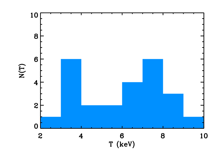
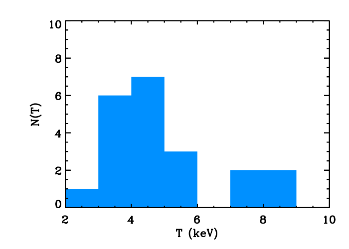
a)                                                                          b)

Figure 1: The distribution of clusters with revised temperatures in the Henry & Arnaud sample, HA91 (left panel). The right panel shows the histogram of the 21 clusters in the Edge et al. (1990) sample, not included in HA91.

In order to determine the temperature function, it is important to have a well controlled sample of clusters. The knowledge of the selection function is therefore critical. For instance, the completeness of the Edge et al. (1990) sample (hereafter E90) was questioned by HA91, and in fact the difference between the E90 and HA91 temperature functions is striking. We therefore re–examine these two samples, although the revised version of HA91 appears to be closer to E90. Rather than plotting the temperature function, we directly examine the histogram of the number of clusters in temperature bins for each sample. In Figure 1a, we show the histogram of the revised temperatures in the HA91 sample, while in Figure 1b, we give the corresponding histogram for the E90 clusters not present in the HA91 sample; this latter will be referred to as the E-HA sample. Comparison of the two histograms clearly reveals a striking difference: there is an apparent deficit of clusters with $T\sim 4-6$ keV in the HA sample as compared to E-HA. Obviously, the smaller number of 4 keV clusters present in the HA sample leads to a lower number density. This is of critical importance in the theoretical modeling, because the abundance of 4 keV clusters is crucial in determining the amplitude of the fluctuations on a 8$h^{-1}$Mpc scale (for $\Omega_{0}=1$). The E-HA set is astonishingly different: the number of clusters reaches a maximum at $T=4$ keV, and then tends to decrease monotonically for higher $T$, meaning that there are relatively fewer hot clusters in the E-HA data set (4 clusters from the E90 sample with poor temperature measurements are not taken into account in E-HA, which adds 3 clusters to the region $T>8$ keV, but this does not change the shape of the histogram). Although statistical analysis of such a small sample is a hazardous exercise, this difference is highly significant: assuming that the number of clusters found in the HA sample between 4 and 6 keV (4 clusters), the probability to have ten clusters or more in the E-HA sample in the same range is less than $10^{-3}$. When dealing with small samples, one must of course be careful of spurious noise introduced by Poisson statistics. However, using different tests we always find this difference significant at a confidence level greater than 95%. It is difficult to understand the origin of such a difference: both samples are X-ray selected and incompleteness is expected to be nearly independent of temperature.

It is possible that the existence of large–scale fluctuations, as can be seen from the visual appearance of the clusters distribution or from the long–range correlation function, indicates that noise due to a finite number of objects may be larger than that expected from Poisson noise.

The comparison we have presented in Fig. 1 clearly calls for a larger, complete flux limited sample strictly X-ray selected. However, only the Rosat All Sky Survey (RASS) would allow the construction of such a sample. The Bright Cluster Survey BCS (Ebeling et al., 1998) and the RASS South (De Grandi et al., 1999b) have just become available at the time of writing, but the lack of temperature information for a significant fraction of these clusters prevents us from using these samples to usefully estimate the temperature distribution function. Recently, M98 provided a new local temperature function based on the XBACS sample (Ebeling et al, 1996). XBACS is an essentially complete, flux-limited X-ray sample of Abell clusters. In principle, the restriction to Abell clusters implies that the sample is possibly incomplete. There are three possible sources of incompleteness: i) low mass (i.e., low temperature) clusters may be missing because they are not rich enough to be selected by the Abell criteria; ii) distant clusters could be missed because at large redshifts clusters hardly meet the Abell criteria; iii) there is a significant difference between the optical based Abell criteria and those based on X-ray fluxes. M98 restricted his sample to the redshift range $0.04\leq z\leq 0.09$, the lower limit being imposed by ASCA. This redshift restriction eliminates intrinsically faint clusters from his sample. M98 corrected for this incompleteness by using a weight to compensate for the selection function. The resulting temperature function is noticeably higher than previous estimates, although it is claimed to be consistent with them. However, the correction procedure could introduce a systematic error in the derived abundance of cool clusters as we will see in the next section.

3 The present sample

Cluster	z	$T_{X}$1	$L_{X}$2	$s_{X}$3	Ref4.
Virgo	0.0036	2.2${}^{+0.1}_{-0.1}$	1	82.0	6,10
A1060	0.0114	3.25${}^{+0.1}_{-0.1}$	0.47	7.	4,1
A3526	0.0109	3.54${}^{+0.1}_{-0.1}$	0.83	19.	8,1
A262	0.0161	2.15${}^{+0.1}_{-0.1}$	0.55	4.8	4,1
A3581	0.02	2.0${}^{+0.1}_{-0.1}$	0.57	2.9	5,1
A1367	0.0215	3.55${}^{+0.1}_{-0.1}$	1.63	8.3	4,1
A1656	0.0232	8.2${}^{+0.1}_{-0.1}$	7.21	31.6	9,1
A4038	0.029	3.3${}^{+2.6}_{-1.3}$	1.9	5.27	2,1
A2199	0.0309	4.5${}^{+0.1}_{-0.1}$	3.65	9.5	7,1
A496	0.032	4.1${}^{+0.1}_{-0.1}$	3.54	7.5	4,1
A2634	0.0321	3.7${}^{+0.3}_{-0.3}$	0.94	2.3	4,1
A2063	0.0337	3.7${}^{+0.1}_{-0.1}$	2.03	3.7	4,1
A2052	0.0348	3.1${}^{+0.3}_{-0.3}$	2.52	4.7	2,1
Cl0336	0.0349	3.${}^{+0.1}_{-0.1}$	5.87	8.76	4,1
A2147	0.0356	4.9${}^{+0.3}_{-0.3}$	2.84	5.3	4,1
A576	0.0381	4.3${}^{+0.5}_{-0.4}$	1.39	2.24	2,1
0422–09	0.039	2.9${}^{+0.5}_{-0.4}$	2.∗	3. ∗	2,2
A3571	0.0391	6.9${}^{+0.3}_{-0.3}$	7.36	10.9	3,1
A2657	0.04	3.7${}^{+0.3}_{-0.3}$	1.6	2.33	3,1
A2589	0.0416	3.7${}^{+0.6}_{-0.6}$	1.86	2.5	6,1
A119	0.044	5.8${}^{+0.4}_{-0.4}$	3.23	3.8	3,1
MKW3s	0.045	3.5${}^{+0.2}_{-0.2}$	3.	3.43	3,3
A1736	0.0461	3.5${}^{+0.4}_{-0.4}$	2.37	2.6	3,1
A3376	0.0464	4.3${}^{+0.6}_{-0.6}$	2.48	2.69	3,1
A3558	0.0478	5.5${}^{+0.3}_{-0.3}$	6.27	6.2	3,1

Cluster	z	$T_{X}$1	$L_{X}$2	$s_{X}$3	Ref4.
A1644	0.048	4.7${}^{+0.8}_{-0.8}$	3.52	3.64	2,1
A4059	0.048	4.0${}^{+0.1}_{-0.1}$	3.09	3.12	4,1
A3562	0.0499	3.8${}^{+0.8}_{-0.8}$	3.33	3.08	2,1
A3395	0.05	4.8${}^{+0.4}_{-0.4}$	2.8	2.65	3,1
A85	0.0518	6.1${}^{+0.2}_{-0.2}$	8.38	7.2	3,1
A3667	0.053	7.${}^{+0.6}_{-0.6}$	8.76	7.3	3,1
A754	0.0534	7.6${}^{+0.3}_{-0.3}$	8.01	12.	6,1
A780	0.05384	3.8${}^{+0.2}_{-0.2}$	6.63	4.8	3,1
A3391	0.054	5.7${}^{+0.7}_{-0.7}$	2.32	2.39	3,3
A3158	0.059	5.5${}^{+0.6}_{-0.6}$	5.31	3.57	2,1
A3266	0.0594	7.7${}^{+.8}_{-0.8}$	6.15	4.8	3,1
A2256	0.0601	7.5${}^{+0.4}_{-0.4}$	7.05	4.9	3,1
A133	0.0604	3.9${}^{+1.6}_{-0.7}$	3.57	2.29	2,1
A1795	0.0616	6.${}^{+0.3}_{-0.3}$	11.1	6.7	3,1
A3112	0.07	4.7${}^{+0.4}_{-0.4}$	7.7	3.6	3,1
A399	0.0715	7.4${}^{+0.7}_{-0.7}$	6.45	2.9	3,1
A2065	0.072	5.4${}^{+0.3}_{-0.3}$	4.95	2.2	3,1
A401	0.0748	8.3${}^{+0.5}_{-0.5}$	9.88	4.26	3,1
A2029	0.0767	8.7${}^{+0.3}_{-0.3}$	15.35	6.16	3,1
A1651	0.0825	6.3${}^{+0.5}_{-0.5}$	8.25	2.7	3,1
A1650	0.085	5.6${}^{+0.6}_{-0.6}$	7.81	2.56	3,1
A2597	0.085	3.6${}^{+0.2}_{-0.2}$	7.97	2.59	3,1
A2142	0.0899	9.${}^{+0.2}_{-0.2}$	20.74	6.14	11,1
A478	0.09	7.1${}^{+0.4}_{-0.4}$	12.95	3.9	3,1
A2244	0.097	7.1${}^{+1.2}_{-1.2}$	9.09	2.28	2,1

¹ in keV
² in 10⁺⁴⁴erg/s ($h=0.5$)
³ in 10^-11erg/s/cm^2
4 the first reference is for temperature, the second for the luminosity
^∗ inferred from a non-ROSAT measurement.

Table 1: X-ray temperatures, 90% uncertainties, ROSAT 0.1–2.4 keV luminosities (h$=0.5$) and fluxes.

${\bf Ref.}$ (1) Ebeling et al. 1996; (2) David et al., 1993; (3) Markevitch, 1998; (4) Fukazawa et al., 1998 (temperature are given with the emission from the central $0.05h^{-1}$Mpc excluded); (5) Johnstone et al., 1998; (6) Arnaud & Evrard, 1999; (7) Arnaud, 1994; (8) Yamashita et al., 1992; (9) Hughes et al., 1993; (10) Ebeling et al., 1998; (11) White et al., 1994;

As it is clearly an advantage to have a survey which is not redshift restricted, we have collected existing information on clusters with $f_{x}\geq 2.210^{-11}$ erg/s/cm² in the ROSAT band 0.1–2.4 keV (and with $|b_{II}|>20^{\circ}$). In practice, most of the clusters were obtained from the XBACS sample complemented by a handful of non-Abell clusters which satisfy our flux requirement (MKW3s, Virgo, Cl0336 and 0422–09). For all these clusters, temperature measurements were found in the literature. In the following analysis, the redshift range is still restricted to $z<0.1$, because of the possible substantial incompleteness of the sample at higher redshifts. Our final sample contains fifty clusters. It is important to examine its completeness.

A classical test for checking the homogeneity of a survey is to use the $V/V_{m}$ test (Schmidt, 1968). Applying this test, we find a mean value of $V/V_{m}$ = 0.490, consistent with a homogenous sample. The plot of $V/V_{m}$ versus temperature given in Figure 2 does not reveal any unexpected trends. The recent availability of the BCS and RASS samples allows us to check this in a more quantitative way: at our chosen flux limit, four clusters in the BCS and RASS1 are not present in our sample (RXJ0419, IIZw108, Z5029, NGC1550). None of these (non-Abell) clusters has a measured temperature, but from their luminosity, only two of them would have a temperature greater than 4 keV. This is consistent with our sample being complete at a level of 95% for $T\geq 4$ keV, while the completeness of the BCS and RASS is estimated to be better than 90%. Therefore, our estimated completeness is 85% and we will treat it as an essentially complete, X-ray selected ensemble of clusters, at least for clusters with temperature greater than 4 keV. It is the largest homogenous sample of X-ray selected clusters currently available for the estimation of the temperature distribution function. Notice that the possible incompleteness of our sample would imply that the inferred temperature function could be an under-estimate.

At redshifts $z\geq 0.04$, our sample is similar to M98. The temperature histograms of both M98 sample and ours are shown in Figure 3. As one can see, the two histograms are nearly identical on the hot end, but differ on the cool end (for $T<5$ keV). This difference is not surprising given the restricted redshift range investigated by M98. However, it is important to investigate the temperature function on the cool end since the number of clusters in the two samples differs noticeably. Although M98 corrected for the incompleteness of his sample, using a larger sample will result in a statistically better estimate with reduced sensitivity to systematics. Such a sample has two main advantages: with a selection in the ROSAT band, we are much less sensitive to the selection function of the 2.–10. keV band, which obviously favors hot clusters (even if in principle the effect of the selection function can be corrected for), and the number of clusters in our sample is twice as large as the HA91 sample, leading to better statistics especially on the cool end ($T\sim 4$ keV). We have examined the temperature histograms for clusters with fluxes in the range $2.2-4.0\;10^{-11}$ erg/s/cm² and those with $f_{X}>4.0\;10^{-11}$ erg/s/cm². We find that these two histograms differ noticeably in the same sense as the HA91 and E-HA samples as discussed previously. The reason of this difference is unclear, but it is clearly not due to the 2.–10 keV selection only. Inspection of the redshift distribution does not provide evidence that this could be due to large–scale structures (although the BCS reveals significant fluctuations around $z\sim 0.05$).

Figure 2: $V/V_{m}$ distribution for clusters in our sample as a function of temperature. No sign of incompleteness can be seen from this plot for clusters with $T\geq 3.5$keV.

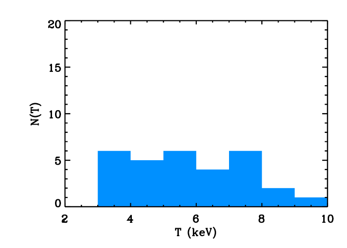
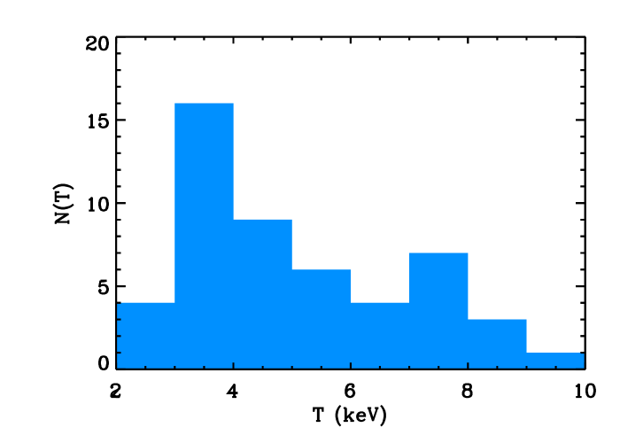
a)                                                                          b)

Figure 3: Same as in Fig. 1 for clusters selected in the ROSAT band. Figure a) represents the distribution of clusters in Markevitch’s sample. b) represents the histogram of the 50 clusters in our sample (XBACS clusters with flux greater than $2.2\;10^{-11}$erg/s/cm² and redshift $z<0.1$). The shapes clearly differ for temperature smaller than 5 keV, while they are nearly identical above. This difference is mainly due to the fact that the Markevitch sample is restricted to redshift $>0.04$.

4 The Determination of the Temperature Function

4.1 The method

Estimation of the luminosity distribution function $\phi(L)$ from a sample for which the selection function is well known is relatively straightforward: the observed number of clusters in the sample $\cal N$ in the luminosity range $(L-L+\Delta L)$ (with $\Delta L\ll L$) is the realization of a stochastic Poisson process with a mean value $\phi(L)V(L)\Delta L$, where $V(L)$ is the volume searched for objects with luminosity $L$. When the selection function $s(z)$ is that of a strictly flux limited sample, $V(L)$ is just the volume $V_{m}$ corresponding to the maximum distance at which the cluster would have been detected. If the selection function $s(z)$ is more complex, then this volume can always be computed as an integral:

$$V(L)=\int_{0}^{+\infty}s(z)dV(z)$$

An unbiased estimation of $\phi(L)\Delta L$ is therefore given by ${\cal N}/V(L)$. In the following, when $B$ is an estimator of some quantity $A$, we use the notation below:

$$A\equiv B$$

According to this notation:

$$\phi(L)\Delta L\equiv{\cal N}/V(L)=\sum 1/V$$

where the summation is performed over all the relevant clusters in the sample. This immediately provides an estimator of the integrated luminosity function:

$$\phi(>L)\equiv\sum_{L_{i}\geq L}1/V(L_{i})$$

We can now recover the standard estimator of the temperature distribution function:

$$N(T)\Delta T=\int_{0}^{+\infty}\phi(L,T)\Delta TdL\equiv\sum_{i}1/V(T_{i})$$ (1)

where the summation is performed over all clusters in the sample in the relevant temperature range. It is important to notice that this estimator is unbiased and fully accounts for the intrinsic dispersion in the temperature-luminosity relation. This procedure may not always be used in practice, if for some region of the parameter space in the sample $V(L)=0$. This is the case for instance, in a flux limited sample which is further restricted to a redshift range. Because of this further restriction, clusters fainter than some intrinsic luminosity may simply not be present in the sample, consequently leading to $V(L)=0$. In this case, the estimation from Eq. (1) is clearly not appropriate anymore. The contribution of the missing clusters can however be estimated, provided the probability distribution of clusters at a given temperature $p(L|T)$ is known. The observed number of clusters is still a Poisson realization of a process whose mean is given by:

$$\int_{0}^{+\infty}\phi(L,T)\Delta TV(L)dL=\int_{0}^{+\infty}N(T)\Delta Tp(L|T)V(L)dL$$

$$=N(T)\int_{0}^{+\infty}p(L|T)\Delta TV(L)dL=N(T)\Delta TV_{s}(T)$$ (2)

The last equality defined $V_{s}(T)$, the effective average volume per cluster of given temperature in the survey. Therefore:

$$N(T)\Delta T\equiv\sum_{i}1/V_{s}(T_{i})$$

This estimator has been used by several authors (Eke et al., 1998; M98). It is unbiased provided that $V_{s}(T)$ is known exactly. In practice, this is of course not the case, since the statistical description of the temperature-luminosity relation and the distribution $p(L|T)$ are not perfectly known, which leads to a source of systematic uncertainty. Consequently, a specific choice of $p(L|T)$ implies a bias in the above estimator. Furthermore, as fewer clusters are actually present in the sample, the Poisson noise increases. It is clear therefore, that this approach should be avoided when possible, unless one can be confident that the resulting uncertainties remain small.

A second important issue concerns errors on temperature measurements: when the true underlying cluster distribution is very steep, positive errors will move many more clusters upwards in temperature than negative errors move hotter clusters downwards, just because of the difference in the intrinsic abundances. This effect has been pointed out by Evrard (1989) for velocity dispersion measurements. A mean statistical correction was applied in the modeling by Eke et al.(1998), while Viana and Liddle (1999a) estimated the magnitude of this effect using a bootstrap resampling technique on Henry’s sample. It is important to realize that when the errors on individual measurements are not identical, a mean correction is not necessarily sufficient, because the weight $1/V_{i}$ varies significantly from one cluster to another. A further problem is that, in principle, the error on the temperature might correlate with the apparent flux of a cluster, as fainter clusters will have lower signal–to–noise and will be those having the larger $1/V_{i}$ as well. In such cases, only a Monte-Carlo reproducing the exact conditions of the observations including the different integration times for the different sources, would in principle allow a complete separation of the various effects of temperature measurement errors.

For the local temperature distribution function, the errors are small enough that the above issue is not a major problem. However, due to larger temperature errors this might be a more critical point for the high–redshift sample. The bootstrap method used by Viana and Liddle (1999a) is certainly well adapted. Another possible way to solve this problem is to use a Bayesian approach: we can take as a prior the distribution function of X-ray temperatures assuming $N(T)\propto T^{-\alpha}$, with $\alpha\approx 5$. Given that a cluster is observed with a measured temperature $T_{0}$ and assuming that the errors are log-normal distributed with a dispersion $\sigma$ (corresponding the observed $1\sigma$ uncertainty), the a posteriori probability that the actual temperature of the cluster be $T$ is given by:

$$p(T|T_{0})\propto N(T)\exp(-(\ln(T)-\ln(T_{0}))^{2}/2.\sigma^{2})$$ (3)

this distribution is also log-normal with the same dispersion but with the most likely temperature $\overline{T}$ shifted compared to $T_{0}$:

$$\overline{T}=T_{0}\exp(-\alpha\sigma^{2})$$ (4)

The above formula may appear strange, because it seems to suggest that a systematic bias exists in the temperature measurements. This is actually not the case, since the observed number of clusters within the sample is rather constant among the different temperature bins. Only the estimated density is biased.

Another effect to take into account for cosmological applications (see section 5.3) when one wishes to relate the mass function to the temperature distribution function, is the dispersion in the $M-T$ relation. The importance of this effect has been discussed by Eke et al (1998). They assumed an intrinsic dispersion of 20%, but neglected the effect of the errors on the actual measurements considering them to be smaller. However, as the effect goes as the square of the error, one should be cautious when dealing with these corrections: in practice, a 20% error (or dispersion in the $M-T$ relation) begins to make a significant difference in the inferred abundance of clusters, while an amplitude of 10% leads to a change that is essentially negligible. In their numerical simulations, Bryan and Norman (1998a) found an intrinsic dispersion of the order of 10% in the $M-T$ relation, twice smaller than the dispersion adopted by Eke et al.(1998) ($\approx 20\%$). In order to understand the bias introduced by these effects (errors on temperature measurements and dispersion in the $M-T$ relation), the Bayesian correction is illuminating: as we have seen, such a correction is equivalent to a modification of the observed temperature, that is to say, the mass-temperature relation in the modeling (this is only an approximation because the Bayesian term depends on the actual slope of the N(T), which might vary with T and redshift, but this is a second order effect). The corrections to implement for observational errors are slightly different in nature though: errors vary from one cluster to another, and also may vary in a systematic way, for instance accordingly to the apparent flux. Furthermore, since the correcting factor varies in a nonlinear fashion, a mean correction is inadequate. Finally, it is worth noticing that errors for high redshift clusters are larger than for the low redshift clusters, and therefore a larger correction is necessary. The practical implication of such a change in the modelling will be discussed is section 5.

4.2 Temperature Distribution Function

We compute the integrated temperature distribution from our sample following the method described in the previous section, i.e. using the estimator:

$$N(>T)\equiv\sum_{\overline{T}_{i}>T}1/V(\overline{T}_{i})$$

The resulting temperature distribution function is plotted as the continuous thin line in Figure 4. A smoothed version is also given. We have also checked that using temperature when the central emission is removed makes negligible difference. For comparison, we have also estimated the temperature distribution function from the HA91 sample, using available updated temperature measurements and the standard estimator (Eq. 1) without the Bayesian correction factor. This temperature distribution is shown as the dotted line in Fig. 4. As one can see, the difference is quite noticeable, in particular around 4 keV, where it is roughly a factor of two. We also show the temperature distribution inferred from the BCS luminosity function (Ebeling et al, 1997) assuming the $L_{x}-T_{x}$ relation as given by OB97. A convenient fit of our temperature distribution function is:

$$N(>T)=1.4210^{-6}h^{3}{\rm Mpc}^{-3}\left(T/4.{\rm keV}\right)^{-1.6}\exp\left(-(T-4.{\rm keV})/2.6\right)$$ (5)

which is plotted in Figure 5. We also show the fit to the temperature distribution function derived by M98. As one can see, we find a larger abundance of cool clusters ($T\leq 4$ keV) than M98 while we have a nearly perfect agreement with the temperature distribution function inferred from the BCS luminosity function.

The difference between our temperature distribution function and previous estimations is striking. The difference with M98 can be easily understood – his sample being restricted to the redshift range $z>0.04$, a significant fraction of faint (and cool) clusters are missing. He has corrected for this incompleteness by a weighting scheme based on an estimated dispersion in the $L_{x}-T_{x}$ relation and following the method discussed in section 4.1. However, in order to properly evaluate such a correction, one needs an accurate estimate of the dispersion in the $L_{x}-T_{x}$ relation, which can only be obtained from a flux–limited sample. The difference with the original HA91 sample is more difficult to understand. One may argue that the difference comes essentially from the band selection ($2-10$ keV ), however as we have already mentioned in section 2, comparison with the E-HA sample suggests another origin. We have therefore divided our sample into two equal sub-samples, corresponding to the brightest and the faintest clusters (in apparent flux). Again, since both samples are X-ray selected (in the same band), they should be statistically equivalent. The corresponding temperature distribution functions are shown in Figure 5. The bright sub-sample leads to a temperature distribution function close to the one based on the HA91 sample. This is not surprising on the high temperature end, since the clusters are almost the same in these two samples. The fact that the temperature distribution functions are almost the same for the cooler clusters as well, indicates that the original HA91 sample does not suffer from any significant bias and that the effects of the chosen band are relatively small. On the other hand, the difference between the faint and the bright samples is quite significant, and the relative abundances of hot and cool clusters is noticeably different. As the difference is marginally 1 $\sigma$, these two samples could be considered as representing two realizations which are slightly in the tail of the distribution, without being really suspicious. Nevertheless, such a difference have some implications in practice as we will see in the next section. The fact that our temperature distribution function is in good agreement with that inferred from the BCS luminosity function is rather encouraging and confirms the absence of any systematics that would undermine our analysis.

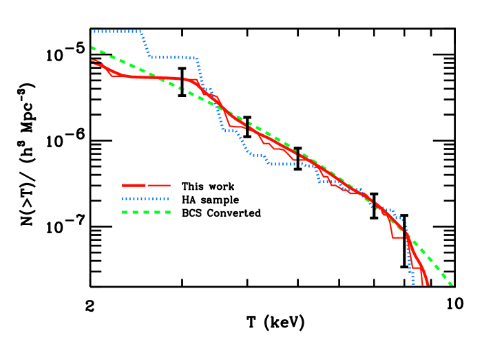
Figure 4: The integrated temperature distribution function inferred from our sample is given by the continuous (red) thin line. A smoothed version is also given (thick line). The dotted line is the same quantity for the original HA91 sample estimated by means of Eq. 1. The dashed (green) line is derived from the BCS luminosity function. The error bars represents the 68% interval for the distribution of the estimator from the bootstrap.

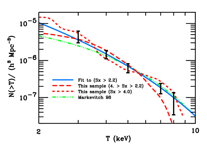
Figure 5: A fit to our temperature distribution function is given by the continuous (red) thick line. The two thick dashed lines correspond to two sub–samples: the short dashed line corresponds to the bright one ($2.210^{-11}>s_{x}>4.10^{-11}$ erg/s/cm²), the long dashed corresponds to the faint sub-sample ($s_{x}>2.210^{-11}$ erg/s/cm²). The long-dashed-3-dotted (green) line is the temperature distribution function from Markevitch (1998).

Differences such those we have found have significant consequences when constraining the spectrum of the fluctuations from the temperature distribution function: a sample in which the abundance of cool clusters is underestimated leads to a too flat spectrum and the amplitude of fluctuations at cluster scales will be also underestimated. All these effects enter as a source of systematic uncertainty in the estimation of $\Omega_{0}$.

4.3 Distribution function of the estimator and Confidence intervals

It is useful to have a statistical description as comprehensive as possible in order to derive strong constraints on models. The number $\cal N$ of clusters in a given temperature range can be regarded as a Poisson realization of mean $\int_{0}^{+\infty}$ $\phi(L)$ V(L) $\Delta$ L. However, the understanding of this quantity requires good information on the $L_{x}-T_{x}$ relation: its shape, its normalization and the distribution function around it. In order to determine the expected distribution of our estimator for $N(T)$, we use a Bayesian bootstrap technique that allows us to avoid the use of a specific $L_{x}-T_{x}$ relation, getting rid of some possible bias thereby introduced. We therefore assume that the distribution of the estimator $\tilde{N}(>T)$ for a given density $N(>T)$ is of the following form:

$$D(\tilde{N})d\tilde{N}=d(\lambda)d\lambda$$ (6)

with $\lambda=\tilde{N}/N(>T)$. We then use a Bayesian bootstrap to reconstruct the distribution function $d$: $10^{4}$ fake samples are built from the original sample, each having the same mean number of clusters, but with a given dispersion to account for Poisson noise. This procedure was used to find the distribution function of the estimator of $N(>T)$, as well as of the estimator for $N(>T_{1})-N(>T_{2})$. The latter quantity is easier to handle with in a statistical analysis, as different temperatures can be chosen in such a way that the measurements are independent quantities (typically $N(>T_{1})-N(>T_{2})$, $N(>T_{2})-N(>T_{3})$,…). We found that a $\chi^{2}$ distribution function fits quite well the distribution function of the estimator, provided that the number of degrees of freedom is left as a free parameter (and is not necessary an integer). An example is given in Figure 6. As one can see, the $\chi^{2}$ distribution provides an adequate fit to the overall distribution. From this we can infer confidence intervals on the density. The error bars given in Figure 4 reflect the 68% range of the value of the estimator of the density of clusters.

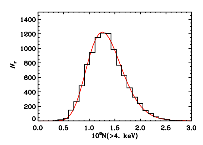
Figure 6: The finite size of the sample implies that our estimate of the abundance of clusters has some uncertainty. The distribution of values that our estimator can take, given the sample we have, is estimated by a Bayesian bootstrap. Here we illustrate the histogram of the values taken by our estimator of the abundance of clusters at present epoch with temperature above 4 keV . A convenient analytical fit of this distribution is also shown: a $\chi^{2}$ distribution with 6 degrees of freedom.

5 Cosmological Applications

5.1 Mass-temperature relation

In order to relate the observable properties of clusters to their mass, physical correlations are necessary. As discussed in the introduction, the temperature of the X-ray gas is probably the most convenient cluster mass estimator. Kaiser (1986) developed the scaling arguments which are essential to this approach (they were already used in 1980 in the pioneering by Perrenod, 1980). Some of the scaling arguments are exact, and they are remarkably powerful. In an Einstein–de Sitter universe with initial fluctuations described by a power–law spectrum, the only process acting is gravity and therefore for the physics of the gas, scaling arguments will hold as long as no other mechanism plays an important role (like cooling or bulk heating). In such a situation, the only possible scale of the problem is associated with the non-linear scale, even in the presence of shock heating. This guarantees that the $T-M$ relation for $M_{*}$ clusters follows an exact scaling law (for a given spectrum):

$$T_{*}\propto M_{*}/R*\propto M_{*}^{2/3}(1+z)$$

It is reasonable to expect that such a relation will also hold between different masses forming at a given redshift and that is nearly independent of the power spectrum. However, this remains an approximation as the geometrical aspect of the peaks corresponding to different masses at a given time may differ (due to the difference in the height of the peaks). The same remark applies for two different spectra. Further checks are therefore needed. Analytical modeling of clusters adopting hydrostatic equilibrium is often completed by the isothermal assumption. However, such a mass estimator can be misleading, even when temperature profiles are taken into account (Balland & Blanchard, 1997). A further problem is the fact that a significant part of the pressure support of the gas could come from turbulent motions in the gas (Bryan and Norman, 1998b). Furthermore, the scaling laws are not expected to hold exactly in open models, significant departures may actually exist in this case (Voit & Donahue, 1998). It seems therefore safer to rely on numerical simulations in order to establish the mass-temperature relation. There are several ways to define the mass of clusters, which are not actually objects with well defined and sharp boundaries. Considerable progress has been made in recent years thanks to Navarro, Frenk and White (1996), who showed that clusters are well fitted by a universal profile involving few parameters (which is not what would be expected based on the isothermal hydrostatic $\beta$-model). Still, various definitions of the mass are used, resulting in some confusion when one wishes to make detailed comparisons. The mass of a cluster could be defined as the mass within the so-called virial radius corresponding to a spherical region with a contrast density $\delta=178$ (in the Einstein-de Sitter case). The mass can also be defined by $\delta=200$, $\delta=500$, or by the mass within a fixed physical radius such as the Abell radius or its equivalent in comoving coordinates. As most of the numerical checks of the mass function have been performed at the virial radius, it is certainly safer to estimate the mass at this very radius. The validity of the scaling models has been impressively demonstrated (Evrard 1989), and no noticeable difference has been detected among different spectra, masses and cosmological backgrounds. Furthermore, an intensive comparison of the results from various codes has verified that different numerical techniques do not lead to significant differences in inferred properties (Frenk et al., 1999). This is especially true for the $M-T$ relation. Even the inclusion of a significant energy injection does not introduce significant changes in these relations (Metzler and Evrard, 1998). The recent numerical work of Bryan and Norman (1998a) is certainly the most advanced in this area, and the scaling relations they obtained are impressive (see their figure 4) and convincingly independent of the underlying cosmological model. Their result can be summarized by the fact that the following mass-temperature relation:

$$T_{v}=3.8{\textrm{k}eV}M_{15}^{2/3}(\Omega_{0}\Delta/178)^{1/3}(1+z)$$

(given for $h=0.5$) reproduces well the results of their numerical simulations ($M_{15}\equiv M/10^{15}$ solar masses). The statistical dispersion they found around this relation is only 10%. The slope $2/3$ might not be guaranteed to better than 15%. However, the normalization of the above relation in the various numerical simulations can differ (for instance, Evrard et al., 1996 found a value 20% higher than Bryan & Norman, 1998a, while the mean value obtained by Frenk et al., 1999, is only 5% higher with a 5% dispersion among the various simulations). The existence of turbulence on small scales (Bryan and Norman; 1998b) indicates that one should be cautious on this issue, as the modeling of turbulence is often limited by the resolution of the simulation. Finally, it is important to notice that such masses are 70% higher than what would be inferred from the isothermal hydrostatic equation (Roussel et al., 2000) and more than twice the mass inferred recently from decreasing temperature profiles as considered by M98, or more recently by Nevalainen et al. (1999). In our modeling, we have adopted the above normalization, corrected for the effect of introducing a 10% dispersion in the $M-T$ relation:

$$T_{v}=4.0{\textrm{k}eV}M_{15}^{2/3}(\Omega_{0}\Delta/178)^{1/3}(1+Z)$$

($h=0.5$). We will examine the consequences of any change in this relation.

5.2 Constraining the models

Figure 7: Contours giving the allowed range of values for the amplitude of matter density fluctuations on cluster scales. The continuous line is the 68% contour, the dotted line is the 90% contour, and the dashed line is the contour at 95%.

The local temperature distribution function can be used to constrain the properties of the matter density fluctuations. Although this can also be applied to a non-Gaussian scenario (OB97; Robinson et al., 1999), we will restrict ourselves to Gaussian fluctuation models only. This consists basically in finding the best parameters and confidence intervals from a fit to the temperature distribution function. However, there is a degeneracy between different cosmological models: equally satisfying fits can be obtained in either low- or high–density models (OB92). Nevertheless, the density fluctuation amplitude can be usefully constrained for a given model. It is generally assumed that cluster abundances lead to a determination of the fluctuation amplitude at $8h^{-1}$Mpc and therefore the normalization is communly expressed in term of $\sigma_{8}$. This is not completely correct. In an $\Omega_{0}=1$ universe, the temperature distribution function of clusters does actually provide the normalization of the fluctuations on this scale. This comes from the fact that the mass of a $8h^{-1}$Mpc sphere collapsing today will lead to a 4.5 keV cluster, which is a typical temperature of a moderately rich cluster for which X-ray samples provide a reasonably well established abundance (at least this what the authors now believe!). In contrast, in a low–density universe ($\Omega_{0}\sim 0.3$), a $8h^{-1}$Mpc sphere will produce a 2 keV cluster, for which we actually do not yet have reliable abundance estimates. This is not just a semantic difference, since for a low–density universe ($\Omega_{0}\sim 0.2$), the amplitude of $\sigma_{8}$ could differ by up 50% (OB97). Following Blanchard & Bartlett (1998), we will use the following definition:

$$\sigma_{c}=\sigma(\Omega_{0}^{-1/3}8h^{-1}\textrm{Mpc})$$

and give constraints in terms of $\sigma_{c}$. This has the additional advantage of being independent of the power spectrum: as $\sigma_{8}$ and the power index $n$ are correlated, the uncertainty on $\sigma_{8}$ is larger than on $\sigma_{c}$. In order to illustrate this point we have plotted both quantities in Fig. 8.

Figure 8: Contours giving the range of allowed values for the index $n$ of the primordial matter fluctuation spectrum on cluster scales for a Gaussian distribution function versus the normalization expressed in term of $\sigma_{8}$ (left side) and in term of $\sigma_{c}$ for a density parameter $\Omega_{0}=0.4$. The continuous lines are the 68% contours, the dotted lines are the 90% contours, and the dashed lines are the contours at 95%.

To find parameter constraints, we find the best model according to the following likelihood function:

$${\cal L}=\prod p\left(N(>T_{i},z_{i})-N(>T_{i+1},z_{i})|N_{\{\Omega_{0},n,\sigma_{c}\}}(>T_{i},z_{i})-N_{\{\Omega_{0},n,\sigma_{c}\}}(>T_{i+1},z_{i})\right)$$ (7)

in which $N$ is the measured abundance and $N_{\{\Omega_{0},n,\sigma_{c}\}}$ is the value given by the model, which depends on the density parameter $\Omega_{0}$, the local slope of the power spectrum $n$ and its amplitude specified by $\sigma_{c}$. The probability distribution function $p$ cannot be inferred from first principles and is therefore estimated with our bootstrap procedure. The maximum value of the likelihood has been normalized to unity, and confidence intervals on the parameters were estimated from the contours at ${\cal L}=0.6,0.26,0.13$ corresponding respectively to the 68%, 90% and 95% contours (strictly speaking this holds only for normal distributions). The constraint on the shape of the spectrum $n$ is rather poor. We find a broad range of possible values. The only obvious result is that models with $\Omega_{0}=1$ and $n\sim-1$, representing the standard Cold Dark Matter spectrum, are excluded, as previously found (Blanchard & Silk, 1991; Bartlett & Silk, 1993). The effect of statistical uncertainties on the amplitude of matter fluctuations on cluster scales is quite small, and therefore only a restricted range of values is allowed for a given $\Omega_{0}$. The dependence on $\Omega_{0}$ is weak :

$$\sigma_{c}\approx \>0.6\leavevmode\nobreak\ ^{+0.035}_{-0.025}\>\Omega_{0}^{-0.14}\>(95\%)$$ open case

$$\sigma_{c}\approx \>0.6\leavevmode\nobreak\ ^{+0.035}_{-0.025}\>\Omega_{0}^{-0.18}\>(95\%)$$ flat case (8)

(uncertainties are statistical and are given for $\Omega_{0}=1$). Different values have been published for the amplitude obtained from the cluster normalization. These differences are mostly due to different cluster abundances used. Our normalization is slightly higher than what is often derived from abundances of X-ray clusters (but in better agreement with some normalizations based on optical surveys, e.g., Girardi et al, 1998). This is due to the fact that our number density of clusters at 4 keV is higher than previous estimations and that we used the Bryan and Norman (1998) normalization of the $M-T$ relation which is slightly lower than that of Evrard et al. (1996). Finally, the differences with previous works concerning the dependence on $\Omega_{0}$ come from the fact that we refer to $\sigma_{c}$, which is the normalization on the true cluster scale rather than to $\sigma_{8}$, which depends on the assumed spectrum (for $n=-1.5$ we find $\sigma_{8}=0.96$ in an open $\Omega_{0}=0.3$ universe).

It is interesting to try to evaluate the magnitude of possible systematic uncertainties on $\sigma_{c}$. As we have argued, the local cluster abundance now seems well established, so that we do not expect this to be a source of systematic error larger than the statistical uncertainty already quoted. The remaining dominant uncertainty comes from the use of the Press and Schechter mass function. Different results exist in the literature concerning its accuracy to describe the actual mass function (Lacey & Cole, 1994). Numerical simulations mostly suggest that the mass function is well described by the Press and Schechter formula: for instance, Borgani et al. (1998) have shown that it can be safely used for cluster modeling in arbitrary cosmology.

Figure 9: Contours giving the range of allowed values for the index $n$ of the primordial matter fluctuation spectrum on cluster scales for a Gaussian distribution function. The continuous line is the 68% contour, the dotted line is the 90% contour, and the dashed line is the contour at 95%.

5.3 Estimating $\Omega_{0}$

The determination of the mean density of the universe is obviously a very important goal of observational Cosmology. Although it is fashionable to claim that current data favor a low value, it seems to us that the observational situation has not improved that much since the 1980’s. Indeed, bulk flows on large scales lead to somewhat contradictory results and interestingly enough, fluctuations in the CMB seem to favor flat models and to exclude open ones (Lineweaver et al., 1997; Lineweaver and Barbosa, 1998; Le Dour et al., 2000). Perhaps the most stringent constraint comes from the baryon fraction observed in clusters (White et al, 1993). Still, a firm upper limit on $\Omega_{0}$ is lacking, because of the uncertainties in primordial nucleosynthesis and cluster mass estimates (notice that virial masses estimated from the scaling models with the normalization we adopt are nearly twice as large as those based on hydrostatic estimations!).

The evolution of clusters is known to be a powerful probe of the mean density of the universe (Perrenod, 1980; Peebles et al. 1989). Evolution of the cluster abundance with redshift offers a new pass to $\Omega_{0}$ (OB92, OB97) which is insensitive to the cosmological constant, and above everything else is really a global probe rather than a local one, as it is the case with the classical $M/L$ argument. It has been shown that the EMSS distribution can be modeled equally well within low- and high–density universes, provided that some evolution in the $Lx-Tx$ relation is adopted (OB97). The required evolution depends on $\Omega_{0}$ as follows:

$$L_{x}\propto T_{x}^{3}(1+z)^{B}$$ (9)

with

$$B\sim 4\Omega_{0}-3.$$ (10)

It is important to ask whether this modeling based on limited observational data is robust or not. Since this work, the observational situation has been considerably improved, thanks to the ROSAT satellite. The number counts for X-ray clusters are now available and fall well within the range of the predictions given by OB97. The ROSAT X-ray cluster luminosity function was derived from the BCS sample (Ebeling et al. 1997) and recently confirmed by De Grandi et al. (1999a). This observed luminosity function matches extremely well the one predicted by OB97. Finally, the amplitude of the fluctuations which was normalized to the original HA91 temperature distribution function, is in good agreement with what has been obtained in the present work. This considerably reinforces the strengt of OB97 modeling. Reichart at al. (1999) have recently re-analyzed the EMSS sample and have reached similar conclusions. Furthermore, similar value of $B$ has been obtained by Borgani et al. (1998) from their analysis of the RDCS survey. The determination of $\Omega_{0}$ from the evolution of the $L_{x}-T_{x}$ relation seems therefore possible, and we expect it to lead to reliable estimates. Thanks to the availability of ASCA temperature measurements for a significant number of high–redshift clusters, it has been shown that this relation undergoes at most only a mild evolution (in the positive direction, i.e., high–redshift clusters are more luminous than local ones with the same luminosity; Sadat et al., 1998). Using the relation between B and $\Omega_{0}$ (eq. 9), Sadat et al. (1998) concluded in favor of a high value of the density parameter ($\Omega_{0}\sim 0.8$) with a quoted uncertainty of $0.2$ (this uncertainty only reflects the uncertainty due to the Poisson noise in the EMSS distribution, and does not take into account the uncertainty in the overall modeling).

Thanks to the availability of the first X-ray selected sample of high–redshift clusters with measured temperatures (H97), it is now possible to constrain the density of the universe using directly the evolution of the X-ray cluster abundance to an intermediate redshift. A value of $\Omega_{0}=0.5$ was obtained (H97) (this value has been abusively referred to as a low $\Omega_{0}$.). Eke et al. (1998) who studied in detail the various systematic uncertainties have found a similar $\Omega_{0}$. A higher value of $\Omega_{0}$ has been derived by Viana and Liddle (1999a) who discussed the importance of a proper correction from the uncertainties introduced by temperature measurement errors. Since these authors used a lower local abundance than the one we have inferred from the present work, it is interesting to re-address this question. Our primary goal here is to analyze the consequences of the higher cluster abundance at zero redshift that we derive. We leave to a future work a more complete investigation of the high–redshift sample.

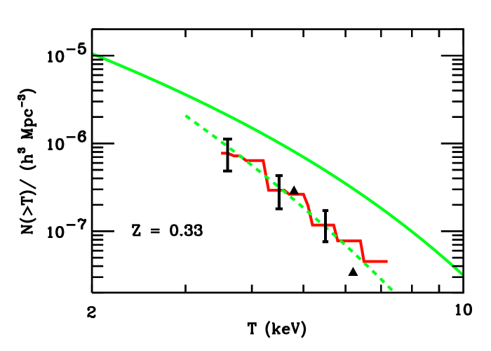
Figure 10: The integrated temperature distribution function at $z=0.33$ inferred from Henry’s sample is given by the continuous thick (red) line (corresponding to the case $\Omega_{0}=0.5$). The two triangles are the estimation from Viana & Liddle (1999a, 1999b) with the original H97 sample. The line is the best fitting model. The continuous grey (green) line is the fit to our local temperature distribution function. The dashed grey (green) line is our best model at $z=0.33$.

We have estimated the temperature distribution function of the distant cluster sample as given by H97, and estimated the suitable volume correction for the various cosmological models. Temperatures were corrected by the Bayesian term. The resulting temperature distribution function is given in Figure 10. For comparison, we have also plotted the temperature distribution function inferred from the local luminosity function. One may worry that our Bayesian correction is adequate. The bootstrap approach followed by Viana and Liddle (1999a) is certainly well adapted to the treatment of measurement errors. We have therefore compared their inferred abundances to ours and found very good agreement (using the 10 original clusters). This confirms that our analytic method provides a correction term which is as good as the bootstrap resampling technique. Our inferred temperature distribution is shown as the thick continuous line in Figure 10.

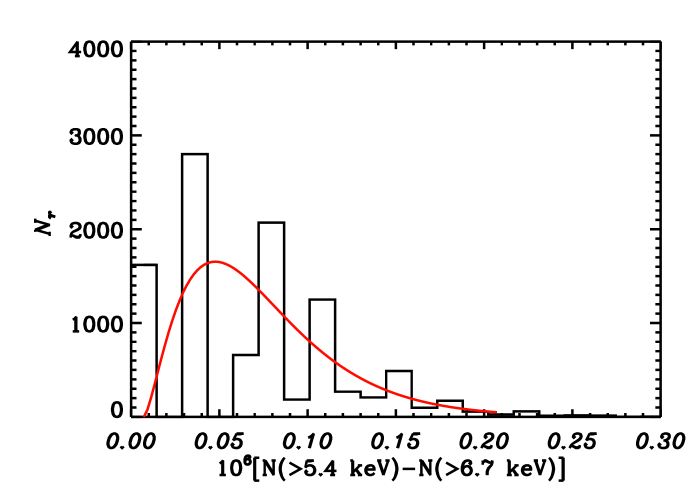
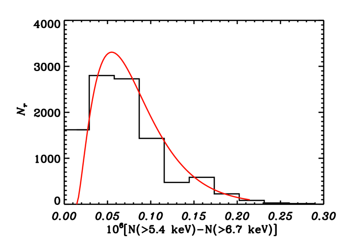
a)                                                         b)

Figure 11: Figure a) represents the histogram of the values taken by our estimator from $10^{4}$ bootstrap resampled samples (as in figure 6). The spikes are real and reflect the fact that the abundance estimation is dominated by a single cluster. In this case, our analytic expression for the distribution function does not work very well (continuous line : $\chi^{2}$ distribution with 1.5 dof). b) represents the distribution function of the estimator with larger bins; in this case the fit is acceptable.

We use the following likelihood function to infer the best-fit value of $\Omega_{0}$:

$${\cal L}=\prod_{i}p\left(N(>T_{i},z_{i})-N(>T_{i+1},z_{i})|N_{\{\Omega_{0},n,\sigma_{c}\}}(>T_{i},z_{i})-N_{\{\Omega_{0},n,\sigma_{c}\}}(>T_{i+1},z_{i})\right)$$ (11)

$$\prod_{j}p\left(N(>T_{j},z_{j})-N(>T_{j+1},z_{j})|N_{\{\Omega_{0},n,\sigma_{c}\}}(>T_{j},z_{j})-N_{\{\Omega_{0},n,\sigma_{c}\}}(>T_{j+1},z_{j})\right)$$

with $T_{i}=\{3.,4.,5.4,6.6,8.,+\infty,z_{i}=0.05\}$ and $T_{j}=\{3.6,4.4,5.5,6.7,8.,+\infty,z_{j}=0.33\}$. The distribution function of the measured abundances was estimated by a Bayesian bootstrap, as discussed in section 4.3. Because of the small number of clusters in the sample, the inferred abundance looks very spiky (see Figure 11a), which simply means that one cluster essentially dominates the statistic. In such a case, our fits are of course never as good as in the case where the number of clusters is larger, but they are reasonably acceptable when the binning in abundance is enlarged (see Figure 11b).

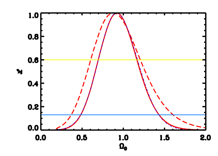
Figure 12: The likelihood function provided by the comparison of the abundances of clusters at $z=0.05$ and $z=0.33$. The continuous line corresponds to the open case, the dashed line corresponds to the flat case. The two horizontal line gives the 1$\sigma$ and 2$\sigma$ confidence interval on one parameter for a gaussian distribution. The dotted-dashed line is a fit by a two-tailled gaussian.

The likelihood function normalized to unity, is given in Figure 12. The most likely values of $\Omega_{0}$ are 0.92 (open case) and 0.865 (flat case). The shape of the likelihood function is very well fitted by a Gaussian, even if the probability functions we have used are significantly non-Gaussian. We can therefore make direct use of this function to give the confidence intervals at the $1\sigma$ level. Our best fitting values are :

$$\Omega_{0}= 0.92^{+0.255}_{-0.215}$$ (open case)

$$\Omega_{0}= 0.865^{+0.35}_{-0.245}$$ (flat case) (12)

This is very consistent with Sadat et al. (1998) value from a completely independent analysis. The constraint we have obtained is quite severe: an open model with $\Omega_{0}<0.49$ is ruled out at the 95% confidence level, a flat model with $\Omega_{0}<0.37$ is ruled out at the same level, conclusions which are in clear disagreement with previous analyses based on the same high redshift sample (H97; Eke et al, 1998). The main differences come from our higher abundance at low redshift and from the fact that we explicitly take into account the effect of temperature measurement errors in the high–redshift sample. Note that Viana and Liddle (1999a) reached values which are consistent with ours. There are a number of other issues that differ in these various analyses and it is important to check whether these differences can result in significantly different values of $\Omega_{0}$. Eke et al. (1998) have analyzed various sources of systematics and concluded that they are not of critical importance. We reach similar conclusions for the effects they have investigated. For instance, we have modified the $M-T$ relation by $\pm$ 20%, which changes $\Omega_{0}$ by $\pm 0.1$. The uncertainty in the validity of the Press and Schechter formalism is also significant but small. Using the revised version by Governato et al. (1998), we found values arround 15% higher. We have checked that our likelihood approach is not biased by applying it to the predicted mean abundance in one model ($\Omega_{0}=0.85$, $n=-1.85$, $\sigma_{c}=0.606$) and found that the best fitting model is ($\Omega_{0}=0.85$, $n=-1.75$, $\sigma_{c}=0.61$). We also have checked that varying the shape of the fitting expression does not change the final likelihood at any appreciable level. After this work was finished, we learned about Donahue & Voit (1999) and Henry (2000) works. The first authors found a significant evolution in the abundance of clusters over the redshift range [0.-0.8], in agreement with Blanchard & Bartlett (1998) and the present work. Nevertheless, they conclude it to be consistent with a lowdensity universe, but simultaneously they found a very flat spectrum $n\sim-2.2$, which is excluded in our analysis based on the local temperature distribution function. Similarly, Henry (2000) found a moderate value of $\Omega_{0}\sim 0.5$ using the HA sample. Indeed, the strongest source of systematic error we found comes from the reference sample we used at zero redshift: using the abundances inferred from the sample limited at the bright end ($f_{x}>4.10^{-11}$ erg/s/cm²) leads to $\Omega_{0}=0.65$ consistent with Eke et al.(1998) and Henry (2000). With the fainter part of our sample ($2.210^{-11}$ erg/s/cm² $<f_{x}<4.10^{-11}$ erg/s/cm²) we obtained $\Omega_{0}=0.98$. The difference obtained just by dividing the sample into two statistically equivalent sub-samples is surprisingly large (althouhg one may not worry of a difference at 1.5 $\sigma$ level): one would expect the uncertainty to come primarily from the high–redshift sample (which comprises only nine clusters) and not from the low–redshift sample.

Our best fit value of $\Omega_{0}$ inferred from the H97 sample is significantly higher than previous estimates from the same sample but it is consistent with the latest optical result by Borgani et al. (1999). It is therefore important to examine the robustness of our analysis. This disagreement with previous results can be due to a higher local abundances of X-ray clusters, and a somewhat different treatment of the bias introduced by the errors at high redshift. As we have already argued, it seems unlikely that our local sample leads to a significant overestimation of the local temperature distribution function. In fact, one could argue that we may underestimate the actual $N(T)$, because of the possible incompleteness of our sample. However, regarding the agreement between our local temperature distribution function and what can be inferred from the luminosity function this is rather unlikely. The high redshift sample might be more worrisome. As we have seen, a systematic difference may exist between two samples, leading to larger differences in $\Omega_{0}$ than expected from Poisson noise. It is therefore conceivable that the high redshift sample is a statistical fluke. For instance, Eke et al. noticed that the temperature distribution within the redshift bin [0.3–0.4] in the original Henry’s sample is statistically surprising as 9 of the clusters lie in the range [0.3–0.35] (now 8 are left). Another possibility is that high–redshift clusters are more massive than what one would infer from their apparent temperature (averaged over the luminosity which comes essentially from the core region). This could be possible for instance, if high–redshift clusters are more often dominated by cooling flows (or if the selection procedure favors cooling flow clusters), making them appear cooler than they actually are and producing an apparent evolution in the $M-T$ relation. At the same time, in order not to produce an evolution in the $L-T$ relation (not seen in the data), these high-z clusters would have to be fainter. This is not very compelling, since cooling flows are expected to increase the X-ray luminosity.

Another potential problem in the above determination of the density parameter is the quality of the EMSS sample: if the selection function is not well understood, it could be that the sample is missing a significantly larger fraction of the cluster population than expected. Indeed, clusters selection in EMSS is rather problematic, as the detection algorithm was designed to detect point sources. A mean correction for extended sources was applied (see Gioia and Luppino, 1994 and OB97 for more details), but one may nonetheless worry that this procedure is not well controlled. However, the deficit of high-z clusters observed in Figure 10 is of the order of 2 to 3. The possibility that the EMSS selection procedure could have missed clusters to such an extent seems unlikely. Furthermore, the modelling by OB97 predicted number counts which are subsequently seen to be in good agreement with available ROSAT counts argues against significant incompleteness of the EMSS sample. An other potential problem could be a systematical bias in the EMSS fluxes. No evidence has been found by Nichol et al. (1997). However, Ebeling et al. (1999) claim that a 40% offset in flux exists, which could explain half of the observed dimming. This possibility does not seem very appealing, because it would imply a very significant evolution in the $L_{x}-T_{x}$ relation. In order to get rid of possible limitations of the EMSS sample, it will clearly be very important to see whether consistent results could be obtained from ROSAT selected samples of X-ray clusters.

6 Conclusion

The local temperature distribution function of X-ray clusters is an important tool for cosmology and can provide direct information on the dark matter distribution. It is therefore essential to have a good estimation of the local temperature distribution function. Furthermore, such a sample is of crucial importance as a reference sample in order to properly evaluate the evolutionary properties of the cluster population and for other cosmological applications. We have provided a new estimate of the temperature distribution function for local clusters, based on a large sample of X-ray clusters with measured temperatures. This sample is essentially flux limited and we have argued that it is likely to be reasonably representative with a completeness estimated to 85%. We found an appreciably higher abundance of clusters than previous estimates, but in good agreement with the abundance inferred from the luminosity function and optical data. We have used the sample to study the statistical properties of the matter density fluctuations and obtained results consistent with previous works, although we obtained a normalization slightly higher, $\sigma_{8}\sim 0.6$ for $\Omega_{0}=1.$ than previously found from X-ray clusters due to our higher abundance of 4 keV clusters. Probably the most important application of this new temperature function concerns the determination of the density parameter via the test of the evolution of the cluster abundance with redshift. In order to apply this test, we have used the Henry’s sample which provides for the first time a direct estimation of the temperature distribution function at a non-zero redshift. We have found a clear indication that the abundance of clusters was smaller at the epoch corresponding to $z\sim 0.33$ consistent with Donahue and Voit (1999). Using a likelihood approach, we inferred a high value of $\Omega_{0}\sim 0.9\pm 0.2$. Low–density open universes ($\Omega_{0}\leq 0.49$) are excluded at the 2 $\sigma$ level. The exclusion region is nearly as severe in the flat case: $\Omega_{0}\leq 0.37$ models are excluded at the 2 $\sigma$ level. This result is entirely consistent with other independent analyses of the EMSS sample (Sadat et al., 1998; Reichart et al., 1999). We therefore confirm that the abundance of X-ray clusters as inferred from the EMSS favors a high–density universe. We have pointed out that this result is also consistent with what is known from existing ROSAT samples, although the situation is not as clear as in the case of the EMSS sample. It is important to keep in mind that the present method is one of the very few cosmological probes of $\Omega_{0}$ that is not based on local estimates, but is rather global in nature. However, given the importance of the conclusion, we believe that it should still be considered with caution. Our study of the local temperature distribution function demonstrated that systematic uncertainties could be more important than expected. It is therefore essential to perform this test using an entirely different and independent sample. Temperature measurements with XMM of ROSAT selected clusters will allow to obtain such a sample. The application of the cosmological test will then probably lead to a more definitive conclusion concerning the mean density of the universe.

References

- (1) Arnaud, M. 1994, Cosmological Aspects of X-ray Clusters of Galaxies, W.C.Seitter ed., NATO ASI Series, Vol. 441, 197
- (2) Arnaud, M. & Evrard, A.E. 1999, MNRAS, 305, 661
- (3) Bahcall, N.A. & Fan, X., 1998, ApJ, 504, 1
- (4) Balland, C. & Blanchard, A. 1997, ApJ, 497, 541
- (5) Barbosa D., Bartlett J.G., Blanchard A. & Oukbir, J. 1996, A&A, 314, 13
- (6) Bartlett, J.G. 1997, Proceedings of the 1st Moroccan School of Astrophysics, ed. D. Valls-Gabaud et al., A.S.P. Conf. Ser., vol. 126, p. 365
- (7) Bartlett, J.G. & Silk, J. 1993, ApJL, 407, L45
- (8) Blanchard, A. & Bartlett, J. 1998, A&A, 314, 13
- (9) Blanchard, A., Bartlett, J. & Sadat, R. 1999, CRAS, 327, 318.
- (10) Blanchard, A. & Silk, J. : 1991, proceedings of the Moriond Conference, 1991, Editions Frontières, p93.
- (11) Bryan, G.L. & Norman, M.L. 1998a, ApJ, 495, 80
- (12) Bryan, G.L. & Norman, M.L. 1998b, astro-ph/9802335
- (13) Borgani, S., Rosati, P., Tozzi, P. & Norman, C. 1999, ApJ, 517, 40.
- (14) Borgani, S., Girardi, M., Carlberg, R.G., Yee, H.K.C. & Ellingson, E. 1999, ApJ, 527, 561
- (15) Carlberg, R.G., Morris, S.L., Yee, H.K.C. & Ellingson, E. 1997, ApJ, 479, L19
- (16) Colafrancesco, S., Mazzotta, P. & Vittorio, N. 1997, ApJ, 488, 566
- (17) David et al 1993
- (18) De Grandi, S. et al. 1999a, ApJL, 513, L17
- (19) De Grandi, S. et al. 1999b, ApJ, 514, 148
- (20) Donahue, M. 1996, ApJ, 468, 79
- (21) Donahue, M., Voit, G. M., Gioia, I., Lupino, G., Hughes, J. P. & Stocke, J. T. 1998, ApJ, 502, 550
- (22) Donahue, M., Voit, G. M., Scharf, C. A., Gioia, I., Mullis, C. P., Hughes, J. P. & Stocke, J. T. 1999, ApJ, 527, 525
- (23) Donahue, M. & Voit, G. M. 1999, ApJL, 523, L137
- (24) Ebeling, H., Voges, W., Böhringer, H., Edge, A.C., Huchra, J.P. & Briel, U.G. 1996, MNRAS, 281, 799
- (25) Ebeling, H., Edge, A.C., Fabian, A.C., Allen, S.W., Crawford, C.S. & Böhringer, H. 1997, ApJL, 479, L101
- (26) Ebeling, H., Edge, A.C., Böhringer, H., Allen, S.W., Crawford, C.S. Fabian, A.C., Voges, W. & Huchra, J.P. 1998, MNRAS, 301, 881
- (27) Ebeling, H., Jones, L. R., Perlman, E., Scharf, C., Horner, D., Wegner, G., Malkan, M., Fairley, B.C. & Mullis R. 2000, Ap.J., 534, 133
- (28) Edge, A.C., Stewart, G.C., Fabian, A.C., & Arnaud, K.A. 1990, MNRAS, 245, 559
- (29) Eke, V.R., Cole, S., Frenk, C.S., Henry, P.J. 1996, MNRAS, 298, 1145
- (30) Eke, V.R., Cole, S., Frenk, C.S., Henry, P.J. 1998, MNRAS, 298, 1145
- (31) Evrard, A.E. 1989, ApJ, 341, L71
- (32) Evrard, A.E., Metzler, C.A., Navarro, J.F. 1996, ApJ, 469, 494
- (33) Fabian, A.C. Crawford, C. S., Edge, A. C., Mushotzky, R. F. 1994, MNRAS, 267, 779
- (34) Frenk, C.S., White, S.D.M., Efstathiou, G., & Davis, M. 1990, ApJ, 351, 10
- (35) Frenk, C.S. et al. 1999, ApJ, 525, 554
- (36) Fukazawa, Y., Makishima, K., Tamura, T., Ezawa, H., Xu, H,Ikebe, Y., Kikushi,K., Ohashi, T. 1998, PASJ, 50, 187.
- (37) Gioia, I.M., Luppino, G.A. 1994, ApJS, 94, 583
- (38) Girardi M., Borgani S., Giuricin G., Mardirossian F. Mezzetti, M. 1998, ApJ, 506, 45
- (39) Governato F., Babul, A., Quinn, T., Tozzi, P., Baugh, C. M., Katz, N.& Lake, G. 1999, MNRAS, 307, 949
- (40) Hattori, M. & Matsuzawa, H. 1995, A&A, 300, 637
- (41) Henry, J.P. & Arnaud, K.A. 1991, ApJ, 372, 410
- (42) Henry, J.P. 1997, ApJ, 489, L1
- (43) Henry, J.P. 2000, ApJ, 535, 350
- (44) Hughes, J.P., Butchler, J.A., Stewart, G.C. & Tanaka, Y. 1993, ApJ, 404, 611
- (45) Johnstone, R.M., Fabian, A.C. & Taylor, G.B. 1998, MNRAS, 298, 854
- (46) Kaiser, N, 1986, MNRAS, 222, 323
- (47) Kruse, G. & Schneider P. 1999, MNRAS, 302, 821.
- (48) Lacey, C. & Cole, S. 1994, MNRAS 271, 676
- (49) Le Dour, M., Bartlett, J.G., Douspis, M. & Blanchard, A. 2000, astro-ph/0004283, submitted to A&A
- (50) Lineweaver, C., Barbosa, D., Blanchard, A. & Bartlett, J. 1997, A&A, 322, 365
- (51) Lineweaver, C. & Barbosa, D. 1998, ApJ, 496, 624
- (52) Markevitch, M. 1998, ApJ, 504, 27
- (53) Metzler, C.A. & Evrard, A.E. 1997, astro-ph/9710324
- (54) Mushotzky R. F. & Scharf C. A. 1997, ApJ, 482, L13
- (55) Navarro, J. F., Frenk, C.S. & White, S.D.M. 1995, MNRAS, 275, 720
- (56) Nevalainen, J., Markevitch, M., Forman, W.R. 2000, Ap.J., 532, 694
- (57) Nichol, R.C., Holden, B.P., Romer, A.K., Ulmer, M.P., Burke, D.J. & Collins, C.A. 1997, ApJ., 481, 644
- (58) Perrenod, S.C. 1980, ApJ, 236, 373
- (59) Oukbir, J. & Blanchard A. 1992, A&A, 262, L21
- (60) Oukbir, J. & Blanchard A. 1997, A&A, 317, 10
- (61) Oukbir, J., Bartlett, J.G. & Blanchard, A. 1997, A&A, 320, 365
- (62) Peebles, P. J. E., Daly, R. A. & Juszkiewicz, R. 1989, ApJ, 347, 563
- (63) Press, W.H. & Schechter, P. 1974, ApJ, 187, 425
- (64) Reichart, D.E. et al, 1999, ApJ, 518, 521
- (65) Robinson, J., Gawiser, E. & Silk, J. 2000, Ap.J., 532, 1
- (66) Roussel, H., Sadat, R., Blanchard, A. 2000, A&A, submitted
- (67) Sadat, R., Blanchard, A. & Oukbir, J. 1998, A&A, 329, 21
- (68) Schmidt, M. 1968, ApJ, 151, 393
- (69) Viana, P.T.R. & Liddle, A.R. 1996, MNRAS, 281, 323
- (70) Viana, P.T.R. & Liddle, A.R. 1999a, MNRAS, 303, 535
- (71) Viana, P.T.R. & Liddle, A.R. 1999b, electronic proceedings of the conference “Cosmological Constraints from X-ray Clusters”, Strasbourg, France, Dec. 9-11, 1998, http://astro.u-strasbg.fr/amas/proc/proceed.html
- (72) Voit, G.M. & Donahue, M. 1998, ApJ, 500, L111
- (73) White, S.D.M., Navarro, J.F., Evrard, A.E. & Frenk, C.S. 1993, Nature, 366, 429
- (74) Yamashita, K., in Frontiers of X-ray astronomy, Ed. Y. Tanaka, K., Koyama (Universal Academy Press, Tokyo), p.475