Coupled Quintessence

Abstract

A new component of the cosmic medium, a light scalar field or  ”quintessence ”, has been proposed recently to explain cosmic acceleration with a dynamical cosmological constant. Such a field is expected to be coupled explicitely to ordinary matter, unless some unknown symmetry prevents it. I investigate the cosmological consequences of such a coupled quintessence (CQ) model, assuming an exponential potential and a linear coupling. This model is conformally equivalent to Brans-Dicke Lagrangians with power-law potential. I evaluate the density perturbations on the cosmic microwave background and on the galaxy distribution at the present and derive bounds on the coupling constant from the comparison with observational data.

A novel feature of CQ is that during the matter dominated era the scalar field has a finite and almost constant energy density. This epoch, denoted as $\phi$MDE, is responsible of several differences with respect to uncoupled quintessence: the multipole spectrum of the microwave background is tilted at large angles, the acoustic peaks are shifted, their amplitude is changed, and the present 8Mpc$/h$ density variance is diminished. The present data constrain the dimensionless coupling constant to $|\beta|\leq 0.1$.

1 Introduction

The recent evidence in favour of an accelerated cosmic expansion (Perlmutter et al. 1999; Riess et al. 1999) has prompted the theorists to hypothesize components of the cosmic medium additional to the ordinary matter and radiation, whose equation of state is unable to provide the required kinematics. In a flat Universe, the dark energy of such a component should provide roughly 70% of the cosmic density, and should possess an effective equation of state

$$p=(w-1)\rho,$$ (1)

with the present value (Turner & White 1997, Perlmutter et al. 1999, Wang et al. 1999)

$$w\in(0,0.6).$$ (2)

The most obvious candidate, a cosmological constant, which provides $w=0,$ has unappealing features: its value would be one hundred orders of magnitude smaller than dimensionally expected; upper limits from lensing effects barely allows for a $\Omega_{\Lambda}=0.7$ (Kochanek 1995), as would be necessary to reconcile the amount of matter in clusters with the flatness suggested by inflation. The next simplest possibility is perhaps to include in the cosmic fluid a light scalar field. In fact, if the field is light enough to vary slowly during a Hubble time, its potential energy can drive an accelerated expansion, just like during inflation. The varying field equation of state can then be tuned to lie in the observed range: if this is the case, then the scalar field is sometimes denoted in the literature as  ”quintessence”. The scalar field density fraction $\Omega_{\phi}$ can be made to decrease rapidly in the past, so as to pass easily the lensing constraints, and to avoid discrepancies in the primordial nucleosynthesis abundances.

Beside the acceleration argument, a light scalar field is interesting on its own. First, it is predicted by many fundamental theories (string theory, pseudo-Nambu-Goldstone model, Brans-Dicke theory etc.), so that it is natural to look at its cosmological consequences (Ratra & Peebles 1988, Wetterich 1995, Frieman et al. 1995, Ferreira & Joyce 1998). Second, the presence of a scalar field may fix the standard CDM spectrum (Zlatev et al. 1998, Caldwell et al. 1998, Perrotta & Baccigalupi 1999, Viana & Liddle 1998). Finally, even a small amount of scalar field density may give a detectable contribution to the standard CDM scenario, similar to what one has in the MDM model (Ferreira & Joyce 1998).

A scalar field, however, is expected to couple explicitly (that is, beyond the gravitational coupling) to ordinary matter, with a strength comparable to gravity, as put into evidence by Carroll (1998), unless some special symmetry prevents or suppresses the coupling. Such a strong coupling would render the scalar field interaction as strong as gravity, and would therefore have been already detected. However, a residual coupling still below detection cannot be excluded; moreover, if the coupling to baryons is different from the coupling to dark matter, as proposed by Damour et al. (1990), then even a strong coupling is indeed possible. Exactly the same arguments hold if one supposes the quintessence field to be coupled to gravity, rather than to matter, as investigated by Uzan (1999), Chen & Kamionkowsky (1999) and Baccigalupi et al. (1999). Indeed, the two models, although physically different, are related mathematically by a conformal transformation (Wetterich 1995, Amendola 1999a).

The non-minimal coupling of the quintessence field to ordinary matter is therefore worth investigating, especially because the wealth of high-precision data that is near to come allows the intriguing possibility of detecting the coupling on the microwave background and on the present galaxy distribution. In a previous paper (Amendola 1999b, hereinafter Paper I) I showed that a scalar field with an exponential potential (Wetterich 1988, Ratra & Peebles 1988) and an explicit coupling to matter may behave as a kind of hot dark matter component, as was first shown by Ferreira & Joyce (1998) for zero coupling. I showed that the CMB spectrum of the model presents acoustic peaks  displaced from their location without coupling, and that the galaxy power spectrum also bends in agreement to real data. In that case, the field density amounts to at most 20% of the critical density, and the expansion is not accelerated. The interesting feature was that the universe has always been in an attractor solution, independently of the initial conditions.

In this paper I focus instead on accelerated solutions. I explore first the general phase space of a homogeneous quintessence model with the same exponential potential and coupling to matter as in Paper I; I will refer to this model as coupled quintessence, or CQ. Once the phase-space attractors have been identified, two distinct solutions are selected that allow an accelerated epoch, and the density fluctuations on these trajectories are studied by the use of a purposedly modified version of the code CMBFAST by Seljak & Zaldarriaga (1995). The linear perturbations in the uncoupled case has been already studied by Viana & Liddle (1998) and Caldwell et al. (1998). As it will be shown, the coupling introduces several qualitatively new features.

2 Coupled scalar field model

Consider two components, a scalar field $\phi$ and ordinary matter (e.g., baryons plus CDM) described by the energy-momentum tensors $T_{\mu\nu(\phi)}$ and $T_{\mu\nu(m)}$, respectively. General covariance requires the conservation of their sum, so that it is possible to consider a coupling such that, for instance,

$$T_{\nu(\phi);\mu}^{\mu} = CT_{(m)}\phi_{;\mu},$$

$$T_{\nu(m);\mu}^{\mu} = -CT_{(m)}\phi_{;\mu}.$$ (3)

Such a coupling arises for instance in string theory, or after a conformal transformation of Brans-Dicke theory (Wetterich 1995, Amendola 1999a). It has also been proposed to explain ’fifth-force’ experiments, since it corresponds to a new interaction that can compete with gravity and be material-dependent. A coupling that violates general covariance is instead studied in Barrow & Magueijo (1999).

The specific coupling (3) is only one of the possible forms. Non-linear couplings as $CT_{(m)}F(\phi)\phi_{;\mu}$ or more complicate functions are also possible. Also, one can think of different couplings to different matter species, for instance coupling the scalar field only to dark matter and not to baryons, as proposed by Damour et al. (1990) and Casas et al. (1992). Notice that the coupling to radiation (subscript $\gamma$) vanishes, since $T_{(\gamma)}=0.$ Here I restrict myself to the simplest possibility (3), which is also the same investigated earlier by Wetterich (1995) and is the kind of coupling that arises from Brans-Dicke models. In fact, a field with a gravity-coupling term $\frac{1}{2}\xi\phi^{2}R$ in the Lagrangian acquires, after conformal transformation, a coupling to matter of the form (3). In the limit of small positive coupling one obtains

$$C=\kappa\sqrt{\xi}.$$ (4)

where $\kappa^{2}=8\pi M_{P}^{-2}$ and $M_{P}$ is the Planck mass. Moreover, if the Brans-Dicke Lagrangian contains a power-law potential $V(\phi)\sim\phi^{n}$, then the transformed field $\phi^{\prime}$ acquires an exponential potential that, for small positive $\xi$, can be written as

$$V(\phi^{\prime})\sim\exp\left[\left(n-4\right)\kappa\sqrt{\xi}\phi^{\prime}\right]$$ (5)

(see e.g. Futamase & Maeda 1989, Amendola et al. 1993, Amendola 1999a). The CQ model with a linear coupling and an exponential potential that is studied here is therefore conformally equivalent to a large class of Brans-Dicke Lagrangians.

There are several constraints on the coupling constant $C$ along with constraints on the mass of the scalar field particles, reviewed by Ellis et al. (1989) and Damour (1996). The constraints arise from a variety of observations, ranging from Cavendish-type experiments, to primordial nucleosynthesis bounds, to stellar structure, etc. Most of them, however, apply only if the scalar field couples universally to all matter, which is not necessarily the case. The most stringent bound for a universal coupling, quoted by Wetterich (1995), amounts to

$$|C|<0.1M_{P}^{-1}.$$ (6)

If the coupling to dark matter is different from the baryon coupling, then the constraints on the former relaxes considerably, and becomes (Damour et al. 1990)

$$|C|<5M_{P}^{-1}.$$ (7)

It is also to notice that these constraints are local both in space and time, and could be easily escaped by a time-dependent coupling constant. In the following, therefore, $C$ is left as a free parameter.

The constraints from nucleosynthesis refer to the energy density in the scalar component. This has to be small enough not to perturb element production, so that at the epoch of nucleosynthesis (Wetterich 1995, Sarkar 1996, Ferreira & Joyce 1998)

$$\Omega_{\phi}(\tau_{ns})<0.1-0.2.$$ (8)

This bound is satisfied by all the interesting models.

3 Background

Here I derive the background equations in the flat conformal FRW metric

$$ds^{2}=a^{2}(-d\tau^{2}+\delta_{ij}dx^{i}dx^{j}).$$

The CQ scalar field equation is

$$\ddot{\phi}+2H\dot{\phi}+a^{2}U_{,\phi}=C\rho_{m}a^{2},$$ (9)

where $H=\dot{a}/a$ , and I adopt the exponential potential

$$U(\phi)=Ae^{\sqrt{\frac{2}{3}}\kappa\mu\phi}.$$ (10)

The matter (subscript $m$) and the radiation (subscript $\gamma$) equations are

$$\dot{\rho}_{m}+3H\rho_{m} = -C\rho_{m}\dot{\phi}$$ (11)

$$\dot{\rho}_{\gamma}+4H\rho_{\gamma} = 0.$$ (12)

Denoting with $\tau_{0}$ the conformal time today, let us put

$$a(\tau_{0})=1,\quad\rho_{m}(\tau_{0})=\frac{3H_{0}^{2}}{8\pi}\Omega_{m}=\rho_{m0},\quad\rho_{\gamma}(\tau_{0})=\rho_{\gamma 0},\quad\phi(\tau_{0})=\phi_{0}.$$ (13)

Without loss of generality, the scalar field can be rescaled by a constant quantity, by a suitable redefinition of the potential constant $A$. We put then $\phi_{0}=0$. This gives

$$\rho_{m} = \rho_{m0}a^{-3}e^{-C\phi},$$

$$\rho_{\gamma} = \rho_{\gamma 0}a^{-4}.$$ (14)

The Friedman-Einstein equation can be written as

$$H^{2}=\frac{\kappa^{2}}{3}\left(\frac{\rho_{m0}}{a}e^{-C\phi}+\frac{\rho_{\gamma 0}}{a^{2}}+\frac{1}{2}\dot{\phi}^{2}+Ua^{2}\right).$$ (15)

The dynamics of the CQ model has been analysed in Amendola (1999a) in the regime in which either matter or radiation dominates. Here I generalize the analysis to the case in which both matter and radiation are present. As we will see, this introduces some interesting new features. Generalizing Copeland et al. (1997) the following variables are introduced:

$$x=\frac{\kappa}{H}\frac{\dot{\phi}}{\sqrt{6}},\quad y=\frac{\kappa}{H}\sqrt{\frac{U}{3}},\quad z=\frac{\kappa}{H}\sqrt{\frac{\rho_{\gamma}}{3},}$$ (16)

along with the independent variable $\alpha=\log a$. Notice that $x^{2}$ , $y^{2}$ and $z^{2}$ give the fraction of total energy density carried by the field kinetic energy, the field potential energy, and the radiation, respectively, that is $\Omega_{\phi}=x^{2}+y^{2}$ and $\Omega_{\gamma}=z^{2}$. Clearly, the matter energy density fraction is the complement to unity of $x^{2}+y^{2}+z^{2}$. We can rewrite the Eq. (9) and ( 15) as

$$x^{\prime} = \left(\frac{z^{\prime}}{z}-1\right)-\mu y^{2}+\beta(1-x^{2}-y^{2}-z^{2}),$$

$$y^{\prime} = \mu xy+y\left(2+\frac{z^{\prime}}{z}\right),$$

$$z^{\prime} = -\frac{z}{2}\left(1-3x^{2}+3y^{2}-z^{2}\right),$$ (17)

where the prime denotes here $d/d\alpha$ and where I introduced the dimensionless constant

$$\beta=\sqrt{\frac{3}{2}}\frac{C}{\kappa}\quad$$ (18)

(in Amendola 1999a $\beta$ was defined as twice the value above). The parameters $\beta$ and $\mu$ are all we need to completely specify our model. The constraints quoted in the previous section on $C$ become now $\beta<0.025$ for the universal coupling and $\beta<1$ for the dark matter coupling.

The system (17) is invariant under the change of sign of $y,z$ and of $\alpha$. Since it is also limited by the condition $\rho>0$ to the circle $x^{2}+y^{2}+z^{2}\leq 1$, we limit the analysis only to the quarter of unitary sphere of positive $y,z$. The critical points, i.e. the points that verify $x^{\prime}=y^{\prime}=z^{\prime}=0$, are scaling solutions, on which the scalar field equation of state is

$$w_{\phi}=\frac{2x^{2}}{x^{2}+y^{2}}=\rm{const},$$ (19)

the scalar field total energy density is $\Omega_{\phi}=x^{2}+y^{2}$, and the scale factor is

$$a\sim\tau^{\frac{p}{1-p}}=t^{p},\quad p=\frac{2}{3w_{\rm{eff}}}$$ (20)

($t$ being the time defined by $dt=a(\tau)d\tau$). The effective equation of state for the total cosmic fluid, $p_{tot}=(w_{\rm{eff}}-1)\rho_{tot}$ has index

$$w_{\rm{eff}}=1+x^{2}-y^{2}+z^{2}/3=1+\Omega_{\gamma}(w_{\gamma}-1)+\Omega_{\phi}(w_{\phi}-1)$$

(where $w_{\gamma}=4/3$ is the radiation equation of state). As already noticed, a value $0<w_{\phi}<0.6$ is required by observations, while $w_{\rm{eff}}<2/3$ is enough for acceleration.

The system (17) with an exponential potential has up to fifteen critical points, of which only eight can be in the allowed region. They are labelled by a letter that reproduces the classification given in Amendola 1999a, and a subscript that denotes whether beside the field there is a component of matter (subscript M), radiation (R), both (RM) or neither of the two (in which case the energy density is taken up completely by the scalar field; no subscript in this case). The critical points are listed in Tab. I, where $g(\beta,\mu)\equiv 4\beta^{2}+4\beta\mu+18.$ For every value of the parameters $\mu,\beta$ there is one and only one stable critical point (attractor); one or more saddle points can also exist. More details on the phase space dynamics in Wetterich (1995) and Amendola (1999a).

Point $$x$$

Tab. I. Critical points.

The regions of existence and stability of the critical points are summarized in Tab. II . In the table the attention is restricted to the half plane $\mu>0$, since there is complete symmetry under simultaneous sign exchange of $\mu$ and $\beta$. I defined

$$\mu_{+} = \frac{1}{2}\left(-\beta+\sqrt{18+\beta^{2}}\right),$$

$$\mu_{0} = -\beta-\frac{9}{2\beta}.$$

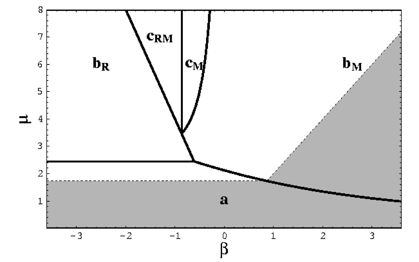
Figure 1: The figure shows the parameter space of the model. Each region is labelled by the critical point that is stable in that region. The shaded area indicates the values for which the attractor is accelerated.

Fig. 1 displays the regions of the parameter space $\mu>0$ in which the various points are stable.

Point Existence Stability Acceleration

$$a$$ ,

never

unstable never

never

never

unstable never

unstable never

Tab. II. Properties of the critical points.

There are only two critical points that admit accelerated solutions, i.e. solutions that satisfy (2): the points $a$ and $b_{M}$. They differ in several important aspects, so we study them separately.

Solutions of type $a$.

The attractor $a$, once reached, brings to zero the matter density. To allow for the observed matter content of the universe, we have to select the initial conditions, if they exist, in such a way that the attractor is not yet reached at the present time, but the expansion is already accelerated. On the positive side, this attractor is accelerated also for small values of the coupling constant. Before discussing in detail the solutions, let us notice that the limit $\beta=\mu=0$ corresponds to the ordinary cosmological constant. Suppose then we put initially the field at zero kinetic energy ($x=0$). A trajectory acceptable from a cosmological point of view should start deep into the radiation era ($z\approx 1$), then enter a matter dominate era ($z\approx 0$), and finally fall into the attractor $a$, the only one still existent for $\beta=\mu=0$, which corresponds to the $\Lambda$-dominated stage. In other words, the path of a ordinary $\Lambda$ universe would be $c_{R}\rightarrow c_{M}\rightarrow a$. A similar sequence of critical points characterizes all the trajectories discussed in the following.

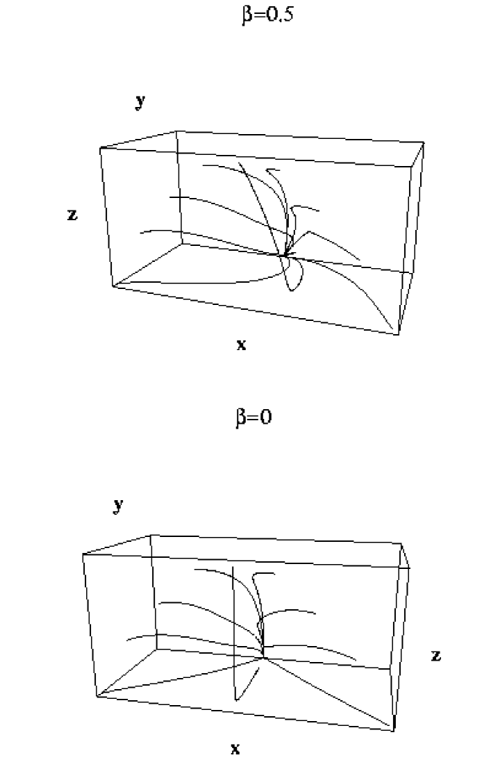
Figure 2: CQ phase space for values that lie in the $a$ region, $\mu=0.1$ and $\beta$ as indicated. The attractor $a$ is the same as in the uncoupled model, but for $\beta\neq 0$ there is a saddle for a non-zero value of the scalar field density. The phase spaces for the values of $\beta$ investigated in this paper are qualitatively similar to the $\beta=0.5$ case. The trajectory that falls almost vertically from top is similar to the background solution effectively employed.

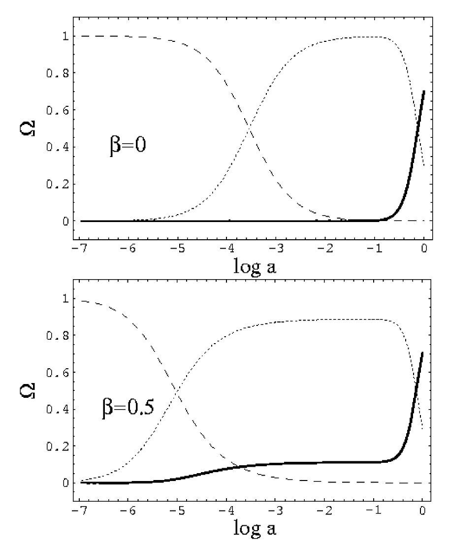
Figure 3: Behavior of $\Omega_{M}$ (dotted line), $\Omega_{R}$ (dashed line) and $\Omega_{\phi}$ (thick line) as a function of $\log(a)$ for $\mu=0.1$ and $\beta$ as indicated. Notice that for CQ there is the transient regime $\phi$MDE in which both the matter and the scalar field energy density are non-vanishing. Notice also that in this case, and for all values of $\beta\neq 0$, the matter-radiation equivalence occurs earlier than in the uncoupled model. For the small values of $\beta$ used for the perturbation calculations, however, this is a small effect.

In Fig. 2 we show the 3D phase space $\left(x,y,z\right)$ of model $a$, with $\beta=0,\mu=0.1$ and $\beta=0.5,\mu=0.1$ . As before, a cosmological trajectory must start in the radiation era ($z\simeq 1$) and has to provide the correct final conditions for $x,y$ and $H.$ Since the scalar field has to start dominating only recently, it is clear that its initial energy density deep in the radiation era has to be very small: in the 3D phase space this means that the cosmic solutions start near $(x,y,z)=(0,0,1)$ , that is, near the unstable critical point $c_{R}$. The trajectories in Fig. 2 that fall almost vertically from top are examples of such cosmic solutions. The attractor of the CQ model is the same as for the uncoupled case, at $\left(x,y,z\right)=\left(-0.033,0.99,0\right)$, but while in the ordinary quintessence case there is a saddle point $c_{M\rm{}}$ at $\left(x,y,z\right)=\left(0,0,0\right)$, in CQ this moves to $\left(x,y,z\right)=\left(2\beta/3,0,0\right)$, on which $\Omega_{\phi}=4\beta^{2}/9$. This appears more clearly from Fig. 3, in which the trend of $\Omega_{m},\Omega_{\phi}$ and $\Omega_{\gamma}$ is reported. The path of this solution is then $c_{R}\rightarrow c_{M}\rightarrow a$, just as in the pure $\Lambda$ model. For $\beta>3/2$, actually, the point $c_{M}$ ceases to exist, but such high values of $\beta$ are anyway unacceptable.

It is to be emphasized that the stage of constant and finite $\Omega_{\phi}=4\beta^{2}/9$ is typical of the CQ model, as it is absent in the limit of zero coupling. Let us call this the field-matter-dominated era, or $\phi$MDE . As we will see, this stage is responsible of most of the differences with respect to ordinary quintessence.

The equivalence time in CQ occurs earlier than in uncoupled quintessence:

$$a_{eq}=\left(\frac{\rho_{\gamma 0}}{\rho_{m0}}\right)^{\frac{3}{3-2\beta^{2}}}.$$ (21)

For the acceptable values of $\beta$, however, this shift has only a minor effect.

Finally, it is to be noticed that the attractor $a$ is independent of the coupling $\beta.$ Then, as the universe at $z\simeq 5$ converges toward the point $a$, the dynamics becomes independent of the coupling. As a consequence, the cosmological probes at $z<5$ , like the type Ia supernovae or the cluster abundance, are not efficient tools for discriminating between ordinary quintessence and CQ.

Solutions of type $b_{M}$.

The attractor $b_{M}$ is a solution for which the matter density and the scalar field share a finite and constant portion of the cosmic energy. For instance, if we put

$$\beta=4.02,\quad\mu=2.68$$ (22)

we get $\Omega_{M}=0.3$ , $\Omega_{\phi}=0.7$ and $w_{\phi}\simeq 0.14,$ well within the requested range. These values, once reached, remain indefinitely constant. The coincidence of similar values of the energy density in the matter and field component is therefore solved, independently of the initial conditions. On the negative side, however, these solutions require a large value of the coupling constant ( $\beta>\sqrt{6/5}$ to obtain $w_{\phi}<0.6$) and are therefore at risk of running into conflict with constraints on the coupling derived from local experiments. The strongest objection to these solutions, however, comes from the simple fact that they lack a matter dominated era, as we will show in a moment.

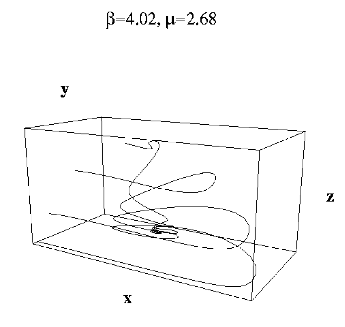
Figure 4: Phase space of CQ for values that lie in the $b_{M}$ region. There is a saddle $c_{RM}$ at $\left(x,y,z\right)\simeq\left(0.12,0,0.95\right)$ that attracts the trajectory that falls from top, similar to the one adopted in the perturbation calculation.

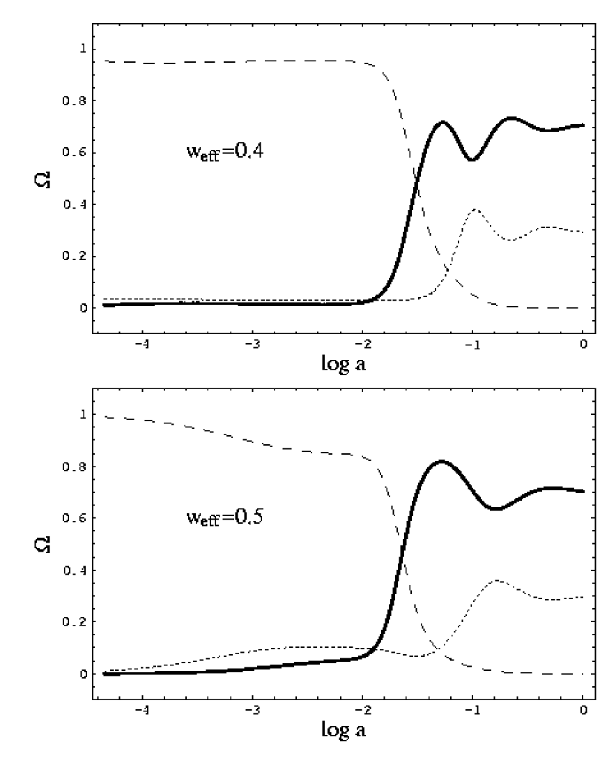
Figure 5: Behavior of $\Omega_{M}$ (dotted line), $\Omega_{R}$ (dashed line) and $\Omega_{\phi}$ (thick line) as a function of $\log(a)$ for  the same parameters as in Fig. 4 (label $w_{\rm{eff}}=0.4$) and for $\beta=\mu=2.37$ (label $w_{\rm{eff}}=0.5$). Notice the transient epoch in which radiation and field share the total energy density (saddle $c_{RM}$).

In Fig. 4 we show the phase space of model $b_{M}$, assuming $\beta=4.02,\quad\mu=2.68$. As can be seen, the phase space is now completely different. The attractor is at $\left(x,y,z\right)=\left(-0.22,0.81,0\right)$. The trajectory that falls from top is again similar to the one used in the perturbation calculations. As can be seen better in Fig. 5, there is a transient near the saddle point $c_{RM}$ , here at $\left(x,y,z\right)\simeq\left(0.12,0,0.95\right)$. In Fig. 5 the evolution of $\Omega_{m},\Omega_{\phi}$ and $\Omega_{\gamma}$ in two cases is displayed, one for which the present value of $w_{\rm{eff}}$ equals 0.4, for which $\beta$ and $\mu$ must be chosen as above, and the other for $w_{\rm{eff}}=0.5,$ which requires $\beta=\mu=2.37$.  In both cases we can see the transient $c_{RM}$ , characterized by $\Omega_{\phi}=1/(4\beta^{2})$   and $\Omega_{M}=1-1/(2\beta^{2})$, followed by the decay of the radiation component and the stabilization of the field and matter to their final values. The path of this solution is then $c_{R}\rightarrow c_{RM}\rightarrow b_{M}$, in contrast with the solutions of the type $a$. As already remarked, such a trajectory is possible only for $\beta\neq 0$. The most conspicuous features here is that the radiation dominates until recently ($z\simeq 50$) and the matter dominated era is absent. As is intuitive, such behavior is catastrophic for the growth of the fluctuations: when a fluctuation mode reenters the horizon, in fact, is suppressed first by the long RDE,  and then by the accelerated expansion. As a consequence, the present $\sigma_{8}$ is unacceptably small, of the order of $10^{-4}$ for COBE normalized spectra. Unless some mechanism other than gravitational instability powers the fluctuations, the trajectories of type $b_{M}$ are precluded. In the following we restrict therefore our attention to solutions of type $a$.

This concludes the analysis of the homogeneous solutions of CQ. It is to be stressed that we considered all the possible accelerated solutions. As in the next section we will span all the range of $\beta$ and $\mu$ that yield cosmologically acceptable solutions of type $a$, we can consider exhausted the analysis of CQ for exponential potentials and linear coupling.

4 Perturbations along solutions $a$

We now proceed to study the evolution of the perturbations in the coupled quintessence theory. The equations of the perturbations in the synchronous gauge have been derived and discussed at length in Paper I and will not be repeated here. In that case it was shown that several important features of the perturbation evolution could be derived analytically, since the background evolution was always on one of the attractor, and thus particularly simple. The same occurs here, at least in some cases. As described in Paper I, all the results presented below have been obtained by modifying the code CMBFAST of Seljak & Zaldarriaga (1996).

The key fluctuation equation in Paper I was the evolution of the sub-horizon perturbations in the MDE regime, the only situation in which the evolution differs from the pure CDM case. For CQ, this regime is actually the $\phi$ MDE introduced above. Let us note first that along any attractor with $x=x_{a}$ one has, from Eq. (16)

$$\phi=\frac{\sqrt{6}x_{a}}{\kappa}\log a.$$ (23)

Denoting with $\delta$ the fluctuation in the matter component, we derived in Paper I an equation for sub-horizon modes in MDE along an attractor that can be rewritten as follows:

$$\ddot{\delta}+H\left(1+2x_{a}\beta\right)\dot{\delta}-\frac{3}{2}H^{2}\Omega_{M}\delta\left(1-\frac{4\beta^{2}}{3}\right)=0.$$ (24)

As we noticed in the previous section, the solutions $a$ passes through the $\phi$MDE transient attractor $c_{M}$, before the present $\phi$-dominated epoch. Therefore, from Tab. I, we can substitute $x_{a}=2\beta/3$. It follows that Eq. (24) has a growing solution

$$\delta=Aa^{m},\quad\rm{with}\quad m=1-\frac{4\beta^{2}}{3}.$$ (25)

This shows two important facts: first, the fluctuations in $\phi$MDE are suppressed with respect to the standard CDM behavior ($m=1$), which also holds for the uncoupled quintessence model, for all values of $\beta$; second, the evolution does not depend on the sign of $\beta$. B efore the present time, at $z\simeq 5$, the trajectory deviates from the $\phi$MDE solution, and $\phi$ begins to dominate.

In Fig. 6 the behavior of three density fluctuation wavelengths, calculated numerically with CMBFAST , is shown as a function of the scale factor $a$. I plot $\delta/a$ to enhance the differences among the various cases. It is possible to distinguish four distinct epochs. Let us first follow the intermediate wavelength of Fig. 6. First, the 100 Mpc/$h$ fluctuation grow as $a^{2}$, while it is a super-horizon mode in RDE; then, around $z\simeq 2500$ $(a\simeq.0004)$ , it reenters the horizon and freezes until the $\phi$MDE begins. In uncoupled quintessence ($\beta=0$) the fluctuation grows now as $a$ , as usual; in CQ the growth is instead suppressed as expected from Eq. (25). Finally, around $z\simeq 5$, $\phi$ starts to dominate, the universe accelerates, and the fluctuation growth is definitely suppressed in all cases. The longer wavelength follows the same phases, except that it reenters directly in the $\phi$MDE, and therefore bypasses the freezing stage. The shorter wavelength starts in the plot already inside the horizon, and follows the same $\phi$MDE growth evolution of the other modes.

The same $\phi$MDE attractor solution can be used to derive the location of the first acoustic peak on the CMB. In fact, this depends essentially on the size of the sound horizon $r_{s}$ at decoupling (subscript $d$). We have shown in Paper I that the following approximated law governs the size of the sound horizon along an attractor solution

$$r_{s}=r_{0}\frac{a_{d}^{x_{a}\beta}}{1+2x_{a}\beta}$$ (26)

where $r_{0}=2(a_{d}/3)^{1/2}H_{0}^{-1}$ is the standard sound horizon. Therefore, the multipole location of the first acoustic peak is

$$\ell_{peak} \simeq \frac{2\pi}{r_{s}H_{0}}=\ell_{0}(1+2x_{a}\beta)a_{d}^{-x_{a}\beta}$$ (27)

$$= \ell_{0}\left(1+\frac{4\beta^{2}}{3}\right)a_{d}^{-2\beta^{2}/3}$$ (28)

where $\ell_{0}\simeq 2\pi/(r_{0}H_{0})\simeq 200$ is the standard peak location, and where the second line specializes to the $\phi$MDE attractor $c_{M}$. For instance, $\beta=0.1$ gives a location $\ell_{peak}\simeq 1.06\ell_{0}$ which, at least to a first approximation, is in agreement with the numerical results below. Notice again that the peak displacement is always toward larger $\ell$s, regardless of the sign of $\beta$, contrary to what happened in Paper I along the attractor $b_{M}$. Similar behavior was found numerically by Chen & Kamionkowsky (1999) and Baccigalupi et al. (1999) in Brans-Dicke models. Here, substituting $\beta^{2}=3\xi/2$, we find that the peak shifts approximately as $(1+2\xi)a_{d}^{-\xi}.$

The solution we use as background in this section is, as anticipated, on its way to the attractor $a$. The initial conditions will be chosen so that at the present time (i.e., when $H^{-1}=3000$ Mpc$/h$) we have $\Omega_{m}=0.3$ , $\Omega_{\phi}=0.7$ and $w_{\phi}\simeq 0.$ This implies that at the present time we should have

$$x_{0}\simeq 0,\quad y_{0}=0.837,\quad z_{0}=0.092$$ (29)

independently of $\beta$. We begin by investigating the parameter range:

$$\mu=0.1,\quad\beta\in\left(0,0.15\right)$$

The initial conditions that produce the requested final values have been obtained by trial and errors. Inserting the background solution in the modified CMBFAST code, we obtain the CMB spectra reported in Fig. 7. The other values adopted are

$$h=0.7,\quad\Omega_{b}=0.04,\quad n=1.$$ (30)

It can be noticed that the peaks move to larger multipoles, as expected. Their amplitude is generally reduced, due both to the growth suppression found above, and to the fact that now the COBE normalization at small $\ell$ includes the integrated Sachs-Wolfe (ISW) effect, no longer negligible in CQ, and as a consequence the fluctuation amplitude at decoupling is reduced (see for instance Hu & White 1996). The ISW is also responsible for the tilt at small multipoles. Models with $\beta>0.15$ are already ruled out by CMB observations, while models with $\beta<0.01$ are essentially indistinguishable from uncoupled quintessence. Values smaller than $\beta<0.06$ produce acoustic peaks which are slightly above those for  the uncoupled model. The bound $\beta<0.15$ is already stronger than (7), valid for the coupling to dark matter; the determination of the spectrum with a precision of 5%, within reach of the Boomerang or Maxima experiments will constrain $\beta$ to two decimal digits, better than current constraints to the baryon coupling (6). The effect for $\beta<0.03$, which satisfies the constraint for the universal coupling model, will be distinguishable in the near future.

The reason for the small increase in the acoustic peak that is observed for $|\beta|<0.06$ is not entirely clear. Since the numerical fluctuation growth follows very closely the analytical prediction of Eq. (25) I believe the rise is not a numerical artifact. Notice that for small $\beta$ the $\phi$MDE transient attractor starts just past the decoupling epoch, and thus the analytical expectations based on the $\phi$ MDE solution are not accurate.

The effect of changing $\mu$, within the limit $\mu<\sqrt{3}$ necessary to have acceleration, is minimal, since the trajectories must anyway satisfy the same final conditions. The spectrum for $\beta=0$ is therefore almost identical to the spectrum of a pure $\Lambda$ model with $\Omega_{\Lambda}=0.7$ . Also, as expected from the analytical expressions, the perturbative results are almost insensitive to the sign of $\beta.$ The present analysis therefore spans all the possible accelerated trajectories in CQ with $\Omega_{\phi}=0.7$ that are cosmologically acceptable.

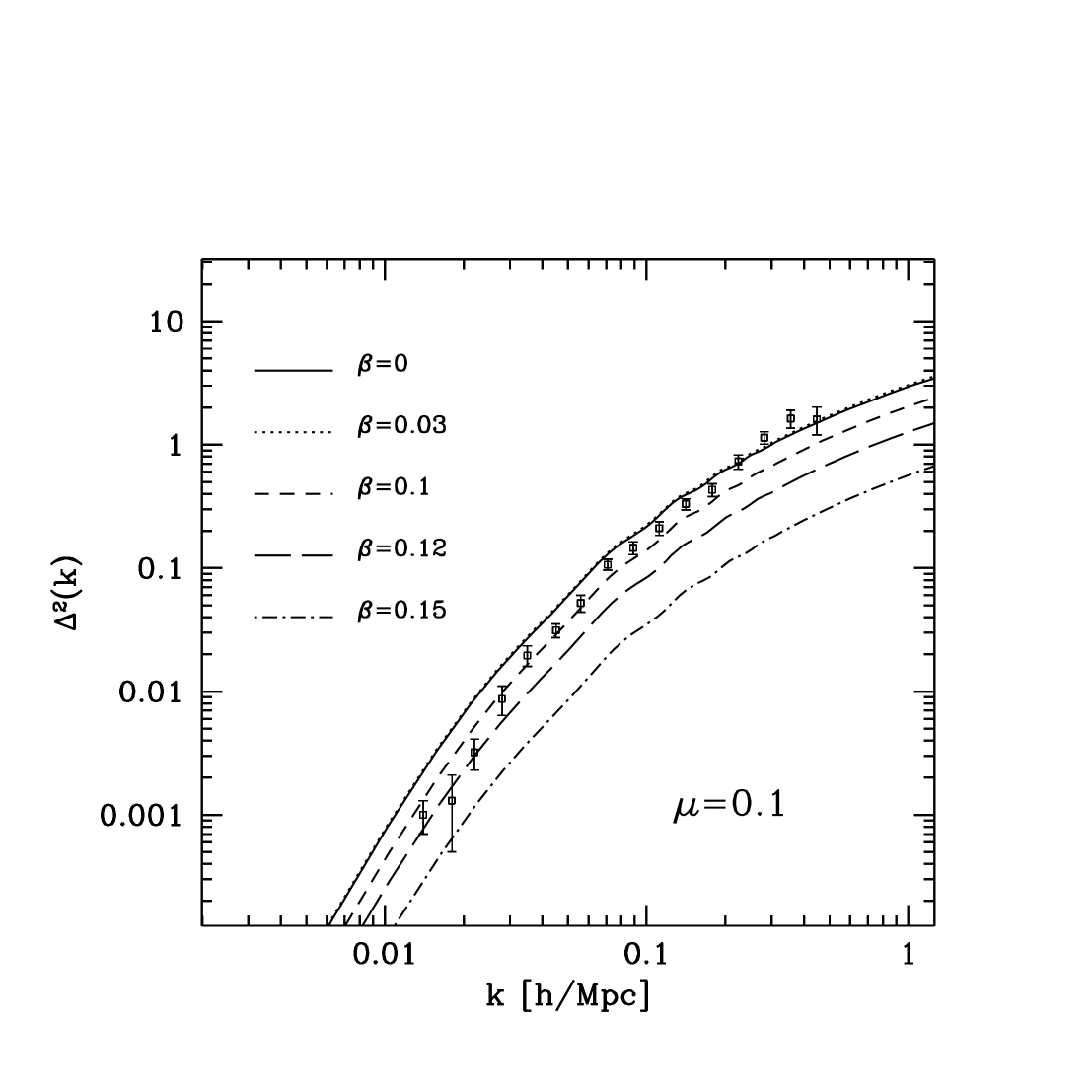
Figure 8: Power spectrum $\Delta^{2}(k)=k^{3}P(k)/(2\pi^{2})$ for the same solutions of type $a$ of Fig.  7. The real galaxy data are from Peacock & Dodd (1994).

In Fig. 8 I report the power spectra $\Delta^{2}(k)=k^{3}P(k)/(2\pi^{2})$ normalized to COBE, compared to the data compiled and corrected for redshift and non-linear distortions by Peacock & Dodds (1994). It can be seen that the slope of the spectrum is in rough agreement with what is observed (the largest discrepancy is for the four smallest scale data points, where non-linearity and redshift distortions are more difficult to correct); a more precise comparison depends on the assumption that the bias between galaxies and dark matter is scale-independent, and on other variables which are not of interest here, like $h$.

The matter fluctuation variance in 8Mpc$/h$ cells $\sigma_{8}$ for a $\Omega_{m}=0.3$ universe should be around unity to fit the cluster abundance (White, Efstathiou & Frenk 1993, Viana & Liddle 1996, Girardi et al. 1998). Wang & Steinhardt (1998) find, for a constant-$w$  model, a general expression for $\sigma_{8},$ that corresponds to $\sigma_{8}\in(0.85,1.25)$ at the 95% c.l., adopting our cosmological parameters. It is found that this is satisfied by $|\beta|\leq 0.1$ , so that this can be taken as the upper limit on $|\beta|$ (see Fig. 9). As found analytically, the suppression of $\sigma_{8}$ with respect to COBE-normalized standard CDM is due to the growth suppression in MDE. Another factor is that now the COBE normalization includes the integrated Sachs-Wolfe effect, no longer negligible. The rise in the CMB spectrum that we observed for small $\beta$ induces via the COBE normalization a similar small rise in $\sigma_{8}$ for the same values, as can be seen in Fig. 9.

A fit to $\sigma_{8}(\beta)$ gives

$$\sigma_{8}(\beta)=\sigma_{8(0)}10^{\left(4.5\beta\right)^{1.5}-\left(6.4\beta\right)^{2}}$$ (31)

where $\sigma_{8(0)}$ refers to uncoupled quintessence, and contains all the dependence on the other cosmological parameters, as well as on the exact COBE normalization scheme (I used here the Bunn & White (1997) normalization implemented in the original CMBFAST code).

5 Conclusion

Soon cosmology will benefit of high-precision data that will allow unprecedented accuracy in testing fundamental theories. Quintessence models add to the battery of cosmological parameters at least two entries, one describing the potential of the field and another its coupling to the rest of the world. So far, the coupling was arbitrarily put to zero, although we know no symmetry condition that implies so. In this paper we let the coupling be non zero, and investigated systematically all the possible trajectories in a flat space that lead to accelerated expansion at the present with $\Omega_{\phi}=0.7$.

The results for the homogeneous theory are applicable also to all Brans-Dicke models with a power law potential, since there is a direct correspondence between our constants $\beta$ and $\mu$ and the Brans-Dicke coupling constant $\xi$ and the potential exponent $n$; from Eqs. (4, 5,18) we have in fact

$$\beta^{2} = \frac{3}{2}\xi,$$

$$\mu^{2} = \frac{3}{2}(n-4)^{2}\xi.$$ (32)

For the fluctuations, the transformation that brings one from the fluctuation quantities in the Jordan frame ( the frame in which the field is coupled to gravity) to those in the Einstein frame (in which the field is coupled to the matter) is more complicated, and a complete treatment is still to be published. However, in the limit in which the fluctuations of the scalar field are small with respect to the fluctuations in the other components the fluctuation fields are conformally invariant; since the CQ field is almost homogeneous due to its light mass, this condition is verified for most of the universe history. As a consequence, it is conjectured that also the perturbative CQ results apply to Brans-Dicke models. The verification of this conjecture is left to future work.

The main feature of the CQ model is the existence of a phase intermediate between the radiation era and the accelerated era, that we denoted $\phi$ MDE. During this era the fluctuations grow less than in an uncoupled model. The $\phi$MDE has three effects on the CMB: the spectrum at low multipoles is tilted, due to the ISW effect; the acoustic peaks are shifted to higher multipoles, due to the change in the sound horizon; and their amplitude is changed in a non-trivial way. On the power spectrum at the present, the main effect is the reduction of $\sigma_{8}$ for large couplings and a very minor enhancement for small coupling.

We found that the potential slope is not efficiently constrained by observations, essentially because the $\phi$MDE is independent of $\mu$. The coupling $\beta$ is on the contrary constrained already by the present data, and is expected to be much more so in the near future, by at least an order of magnitude. From CMB and $\sigma_{8}$ data we can derive the bound

$$|\beta|<0.1$$ (33)

which is stronger than the dark matter constraint of Damour et al. (1990) and not very far from the universal constraint of Wetterich (1995).

Figure 6: Evolution of the matter density contrast $\delta/a$ for three wavelengths, 2$\pi/k=\lambda=$1000 Mpc$/h$ , 100 Mpc$/h$ and 10 Mpc$/h$, for $\mu=0.1$ and various values of $\beta$. Notice the growth suppression for $\beta\neq 0$.

Figure 7: Multipole spectra $C_{\ell}$ (actually we plot $\left[\ell\left(\ell+1\right)C_{\ell}/2\pi\right]^{1/2}\mu$K, as customary) for the solutions $a$. The data are a selection from Tegmark’s home page (http://www.sns.ias.edu/ ~max).

Figure 9: The variance $\sigma_{8}$ versus $\beta.$ The shaded area is the 95% c.l. region that matches the cluster abundance (Wang & Steinhardt 1998).

References

- [1] L. Amendola, Phys. Rev. D60, 043501, 1999a, astro-ph/9904120
- [2] L. Amendola, astro-ph/9906073 (1999), Paper I
- [3] L. Amendola, D. Bellisai & F. Occhionero, Phys. Rev. D47, 4267 (1993)
- [4] C. Baccigalupi, F. Perrotta & S. Matarrese, astro-ph/9906066 (1999)
- [5] J. Barrow & L. Magueijo, Phys. Lett. B447, 246 (1999)
- [6] E. F. Bunn & M. White, Ap.J., 443, L53 (1997)
- [7] R.R. Caldwell, R. Dave, & P.J. Steinhardt, Phys. Rev. Lett. 80, 1582 (1998)
- [8] X. Chen & M. Kamionkowski, astro-ph/9905368 (1999)
- [9] K. Coble, S. Dodelson, J. Frieman, Phys. Rev. D55, 1851 (1997)
- [10] E. J. Copeland, A.R. Liddle & D. Wands, Phys. Rev. D57, 4686 (1997)
- [11] J. Ellis, S. Kalara, K.A. Olive & C. Wetterich, Phys. Lett. B228, 264 (1989)
- [12] P. G. Ferreira & M. Joyce, Phys. Rev. D58, 2350 (1998)
- [13] J. Frieman, C. T. Hill, A. Stebbins, & I. Waga, Phys. Rev. Lett. 75, 2077 (1995)
- [14] T. Futamase & K. Maeda, Phys. Rev. D39, 399 (1989)
- [15] M. Girardi, S. Borgani, G. Giuricin, F. Mardirossian, M. Mezzetti, Ap.J., 506, 45 (1998)
- [16] W. Hu & M. White, A&A, 315, 33 (1996)
- [17] C. S. Kochanek, Ap.J., 453, 545 (1995)
- [18] C.P. Ma & E. Bertschinger, Ap.J. 455, 7 (1995)
- [19] J. Peacock & S. Dodds, MNRAS, 267, 1020 (1994)
- [20] S. Perlmutter et al. Ap.J., 517, 565 (1999)
- [21] F. Perrotta & C. Baccigalupi, Phys. Rev. D59, 123508 (1999)
- [22] B. Ratra, & P.J.E. Peebles, Phys. Rev. D37, 3406 (1988)
- [23] A. G. Riess et al. Ap.J., 116, 1009 (1998)
- [24] S. Sarkar, Rep. Prog. Phys. 59, 1493 (1996)
- [25] U. Seljak & M. Zaldarriaga, Ap.J., 469, 437 (1996)
- [26] J.-P. Uzan, Phys. Rev. D59, 123510 (1999), gr-qc/9903004,
- [27] P. Viana & A. Liddle, Phys. Rev. D57, 674 (1998)
- [28] P. Viana & A. Liddle, MNRAS 281, 323 (1996)
- [29] I. Waga & A. Miceli, Phys. Rev. D59, 103507 (1999)
- [30] L. Wang & P. J. Steinhardt, Ap.J., 508, 483 (1998)
- [31] L. Wang, R. Caldwell, J. Ostriker, & P. Steinhardt, astro-ph/9901388 (1999)
- [32] C. Wetterich, Nucl. Phys. B302, 668 (1988)
- [33] C. Wetterich, A&A, 301, 321 (1995)
- [34] S.D.M. White, G. Efstathiou, C.S. Frenk, MNRAS 262, 1023 (1993)
- [35] I. Zlatev, L. Wang & P. J. Steinhardt, Phys. Rev. Lett. 82, 896 (1999)