A case devoid of bias: ORS voids vs. IRAS voids

Abstract

We present a comparison between the voids in two nearly all sky redshift surveys: the ORS and the IRAS $1.2$-Jy. While the galaxies in these surveys are selected differently and their populations are known to be biased relative to each other, the two void distributions are similar. We compare the spatial distribution of the two void populations and demonstrate the correlation between them. The voids also agree with regard to the overall void statistics – a filling factor of $\approx 0.45$ of the volume, an average void diameter $\bar{d}_{\mathrm{void}}\approx 45h^{-1}\mbox{Mpc}$ and an average galaxy underdensity in the voids $\bar{\delta}\approx-0.9$. Our measurements of the underdensities of the voids in the two surveys enable us to estimate the relative bias in the voids between optical and IRAS samples. We find $(b_{\mathrm{opt}}/b_{\it IRAS})^{\mathrm{void}}\approx 1$, showing that on average there is little – or no – biasing between the two void populations.

1 Introduction

The Optical Redshift Survey (ORS; Santiago et al. 1995) and the Infrared Astronomical Satellite (IRAS) $1.2$-Jy redshift survey [Fisher et al. 1995] comprise an interesting data set pair: both are nearly all-sky surveys (excluding the Galactic plane region: $|b|<20\degr$ for the ORS, $|b|<5\degr$ for the IRAS) and as such are the densest, wide angle, three-dimensional samples currently available for study (at least until the forthcoming release of the IRAS PSC$z$ Redshift Survey, complete to 0.6-Jy – see Saunders et al. 1998). While sampling approximately the same volume, the two surveys differ vis-à-vis the galaxy populations they probe: IRAS and optical catalogues are each compiled using different selection criteria. As a result, IRAS galaxies are biased relative to optically selected galaxies – namely, they are less clustered and underrepresented in cores of galaxy clusters [Strauss et al. 1992].

As such, the two samples were already compared in several studies, e.g., the study of galaxy clustering and morphological segregation in the ORS [Hermit et al. 1996] and the derivation of the ORS-predicted velocity field [Baker et al. 1998], compared with the IRAS $1.2$-Jy gravity field [Fisher et al. 1995]. These works focused on properties derived from the distribution of galaxies in the surveys. In this study, we attempt a different approach, now comparing the distributions of voids in the two surveys.

Voids are the most prominent feature of the large-scale structure of the universe, indeed occupying more than a half of the volume. Thus they are natural candidates for any quantitative large-scale structure study. We have already derived a void catalogue for the IRAS $1.2$-Jy survey [El-Ad, Piran & da Costa 1997], and in this paper we rederive a similar catalogue and present a new void catalogue for the ORS, using a suitably modified version of the void finder algorithm [El-Ad & Piran 1997].

But in addition to this additional void catalogue, the most interesting aspect of this paper is perhaps the comparison between the two void populations: if the galaxies in one survey are biased relative to the other, how does this affect the distribution of the voids? Being almost empty, and using a code which does its best at trying not to depend on the details of the galaxy distribution, voids could prove to be a relatively bias-free statistical probe.

Table 1: ORSd sub-catalogue parameters

Sample	Volume	$N_{\mathrm{gal}}$	$\alpha$	$\beta$	$r_{*}$	$N_{\mathrm{gal}}$	$n_{1}(5)$	$n_{1}(50)$
	Fraction	(total)			(km s-1)	(used)	($10^{-2}h^{-3}\mbox{Mpc}^{3}$)		$\frac{\bar{n}_{{\it IRAS}_{j}}}{\bar{n}_{\it IRAS}}$
(1)	(2)	(3)	(4)	(5)	(6)	(7)	(8)	(9)	(10)
ESGC	0.14	1203	0.50	5.40	10545	684	$20.4$	0.68	1.233
ESO	0.33	1639	0.39	3.22	06425	696	$\phantom{0}6.8$	0.25	0.760
UGC	0.53	1903	0.33	2.75	04085	648	$\phantom{0}9.6$	0.18	1.025

In this paper we derive in a consistent manner and compare void catalogues of the ORS and the IRAS $1.2$-Jy surveys. The paper is structured as follows. In §2 we describe the redshift catalogues we use, and in §3 we briefly review the void finder code and detail the modifications incorporated in order to analyze a survey with a non-isotropic selection function as the ORS. We then introduce the void catalogues (§4) and note some of the familiar voids we identify (§5). In §6 we compare the two void catalogues. Finally, in §7 we summarize our main conclusions.

2 The samples

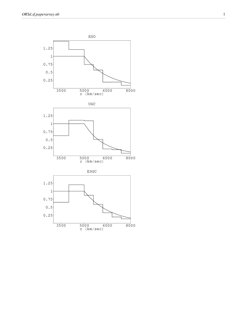
Figure 1: ORSd sub-catalogues radial density profiles for our $50h^{-1}\mbox{Mpc}$ semi–volume-limited samples extending to $80h^{-1}\mbox{Mpc}$. The smooth curves are the calculated selection functions, normalized according to each catalogue’s number density $n_{1}(50)$ (see Table 1, column 9).

From the original redshift catalogues, we construct two semi–volume-limited samples with the same geometry: a sphere extending out to $80h^{-1}\mbox{Mpc}$ with the volume-limited region comprising the inner $\mbox{$r_{0}$}=50h^{-1}\mbox{Mpc}$. The Galactic plane is cut out of our samples eliminating the $|b|<20\degr$ region, as we are limited by the wider ZOA of the ORS; hence our samples extend over 66 per cent of the skies. The volume examined is $1.41\times 10^{6}h^{-3}\mbox{Mpc}^{3}$.

The ORS catalogue [Santiago et al. 1995] contains over 8000 galaxies with redshifts, drawn from three sources – the UGC, ESO and ESGC catalogues. We choose to work with the diameter-limited ORSd sub-sample, as its sky coverage is wider than that of the magnitude-limited ORSm sub-sample (ORSm does not include the ESGC strip). After applying our geometrical cuts and volume-limiting, we end up with 2028 galaxies (Table 1 provides a break down of the galaxy counts per sub-catalogue: column 3 details the original ORSd catalogues, and column 7 details our final sample). The catalogue contains seven $z$-collapsed clusters. Note that since extinction corrections are properly taken into account, the volume limited region is not a perfect sphere – at directions where extinction is not negligible, the volume limited region is shallower having a depth $\mbox{$r_{0}$}/10^{0.2\gamma A_{B}}$. Here $A_{B}(l,b)$ is the extinction in the given direction and passband. $\gamma$ is the extinction correction parameter, for the ORSd being $\gamma_{d}$, the fractional decrease in isophotal diameter with extinction. We used $\gamma_{d}=0.6$ throughout [Santiago et al. 1996].

The various ORSd selection functions were derived as outlined in Santiago et al. [Santiago et al. 1996]. We use a parameterized form for the selection functions [Yahil et al. 1991]:

$$\phi(r)=\left(\frac{r}{r_{s}}\right)^{-2\alpha}\left(\frac{r_{*}^{2}+r^{2}}{r_{*}^{2}+r_{s}^{2}}\right)^{-\beta}$$ (1)

where $\phi(r<r_{s})=1$ and $\alpha$, $\beta$ and $r_{*}$ are free parameters whose best-fit values for our specific samples [Santiago 1998] are given in Table 1.

The IRAS catalogue contains 5321 galaxies complete to a flux limit of 1.2-Jy [Fisher et al. 1995]. The sample we used, selected as explained above, has 1362 galaxies. It is important to note that the two catalogues are not independent – about half of the IRAS galaxies also appear in ORSd, and we have carefully taken this into account in our statistical analysis (§6). All of the analysis is performed in $z$ space.

Table 2: Locations & properties of ORSd voids

ORSd		Equivalent	Total	Location of Centre				Void		Void
Void	Confidence	Diameter	Volume	(Supergalactic Coordinates)				Under-	IRAS $1.2$-Jy	Fit	Identification
Index	Level	[$h^{-1}\mbox{Mpc}$]	[$h^{-3}\mbox{KMpc}^{3}$]	$r$	$X$	$Y$	$Z$	density	Counterpart	$\eta$
(1)	(2)	(3)	(4)	(5)	(6)	(7)	(8)	(9)	(10)	(11)	(12)
1	$>$0.99	64.9	142.9	51.7	$-10.5$	$-35.0$	$-36.5$	$-0.87$	5+9	0.38	EPdC6+7
2	$>$0.99	62.9	130.4	56.5	$-29.3$	$-48.2$	$3.2$	$-0.87$	1	0.58	EPdC5 (Sculptor)
3	$>$0.99	37.7	028.2	41.9	$-8.7$	$-29.0$	$29.0$	$-0.87$	8	0.49	SV2
4	$>$0.99	53.8	081.7	54.2	$-26.0$	$34.7$	$32.5$	$-0.93$	3	0.45
5	$>$0.99	59.7	111.6	57.7	$37.1$	$41.6$	$14.8$	$-0.85$	2	0.49	tip of T1
6	$>$0.98	37.2	026.9	30.5	$-2.9$	$28.8$	$-9.9$	$-0.94$	4+11	0.31	Local–Coma
7	$>$0.98	35.6	023.6	55.5	$-40.9$	$31.7$	$-20.1$	$-0.90$	10	0.48
8	$>$0.98	44.2	045.2	55.3	$9.8$	$29.2$	$45.9$	$-0.86$	6	0.42	CfA2n
9	$>$0.98	46.5	052.6	63.6	$15.5$	$-47.1$	$39.8$	$-0.89$	7	0.60	CfA2s, tip of T2

3 Modifications in the VOID FINDER algorithm

The void finder code used here to derive the void catalogues has been described in detail elsewhere [El-Ad & Piran 1997]. Briefly, the code covers voids using overlapping spheres, iteratively working its way starting from voids containing the largest spheres. Subsequent iterations identify new voids containing smaller spheres and improve the coverage of previously identified voids. Since voids need not be completely empty, an initial phase (wall builder) is used in order to filter out isolated galaxies which are allowed to be in the voids. Corrections are applied in the code in order to handle the observational selection function $\phi(r)$. In a magnitude-limited sample, as we probe deeper we observe a smaller fraction of the galaxy distribution, hence the significance of finding an empty sphere declines with distance. The code corrects for this observational effect by weighing galaxies (during the initial phase) and spheres (during the construction of the voids) according to their distance.

The ORS is more complicated to analyze than the previous surveys we have worked with (SSRS2s and IRAS $1.2$-Jy), since the usage of three different catalogues in its making (and the required extinction corrections) result in a non-isotropic selection function. We modified the void finder code in order to take this into account by appropriately weighing the galaxies and the spheres used to compose the voids. Each galaxy is assigned a weight [Santiago et al. 1996]:

$$W_{i}=\frac{1}{\bar{n}_{j}\phi_{j}(\mn@boldsymbol{r}_{i})}\frac{\bar{n}_{{\it IRAS}_{j}}}{\bar{n}_{\it IRAS}}$$ (2)

where $\bar{n}_{j}$ is the mean number density of ORS galaxies in sub-catalogue $j$ in which galaxy $i$ happens to be located; $\bar{n}_{{\it IRAS}_{j}}$ is the mean number density of IRAS galaxies inside that sub-catalogue; and $\bar{n}_{\it IRAS}$ is the total mean number density of IRAS galaxies (see Table 1, column 10).

The selection function of each sub-catalogue $\phi_{j}(r_{i})$ is usually just a function of the distance $r$, but in order to take extinction into account we adjust it:

$$\phi_{j}(\mn@boldsymbol{r}_{i})=10^{0.2\gamma A_{B}}\phi_{j}(r_{i})$$ (3)

where $A_{B}(l,b)$ are the direction-dependent absorption coefficients [Burstein & Heiles 1982].

Consequently, we calculate a weight for each sphere considered to be a part of a void by volume averaging over the weights of points within each sphere:

$$\bar{W}({\mn@boldsymbol{r}_{\rm centre}},d)=\left(\frac{4\pi}{3}d^{3}\right)^{-1}\int_{\rm volume}W({\mn@boldsymbol{r}})$$ (4)

for a sphere centred on ${\mn@boldsymbol{r}_{\rm centre}}$ with radius $d$.

In order to estimate the underdensity of the ORSd voids we derive $n_{1j}(r_{0})$, the selection function based galaxy number density for each sub-catalogue $j$ up to $r_{0}$. The prescribed number density is $n_{1j}(r_{s})$ where $r_{s}=5h^{-1}\mbox{Mpc}$ (see Table 1, column 8), and we calculate $n_{1j}(r_{0})=n_{1j}(r_{s})\phi_{j}(r_{0})$ (column 9). The actual galaxy number density for $r<r_{0}$ in our samples agrees well with the $n_{1j}(r_{0})$ values, except for ESOd where the actual number density is significantly higher due to the presence of four nearby clusters (Doradus, Hydra, Centaurus and Fornax). See Fig. 1.

For the purpose of calculating the void underdensities: if a void extends over several sub-catalogues, we derive the underdensity in each part of the void separately, and then volume-average the partial underdensities; and if a void extends beyond $r_{0}$ we weigh the galaxies in it using the relevant catalogue’s selection function. Note that since the calculation is done separately in each sub-catalogue $j$ relative to $n_{1j}$, the weight now is simply $1/\phi_{j}$ and no relative density corrections (as in Equ. 2) are required. So the underdensity of a void with volume $V$ containing galaxies at locations $\mn@boldsymbol{r}_{i}$ is:

$$\frac{\delta\rho}{\bar{\rho}}=\sum_{j}f_{j}\left(\frac{\sum_{i}\phi_{j}^{-1}(\mn@boldsymbol{r}_{i})}{V}/n_{1j}(50)-1\right)$$ (5)

where $f_{j}$ is the fraction of the void that happens to be in sub-catalogue $j$.

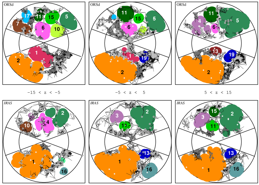
Figure 2: ORSd vs. IRAS slices: for each survey, we present 3 consecutive slices, above and below the supergalactic plane covering the range $-15<Z_{\mathrm{SG}}<15$. The geometry of our samples is indicated by the outer circles, marking the boundary of the samples at $80h^{-1}\mbox{Mpc}$, and the inner circles, marking the volume-limited region at $\mbox{$r_{0}$}=50h^{-1}\mbox{Mpc}$. The excluded ZOA at $|b|<20\degr$ cuts across the samples along $Y_{\mathrm{SG}}=0$. The coloured areas mark the intersection of the three-dimensional voids with the centres of the indicated slices. Voids are numbered as in Table 2 (but the table details only the significant voids); the smaller the void’s index, the more significant it is. Galaxies are marked with dots, and neighboring wall galaxies (i.e., galaxies not allowed to be in voids) are connected with lines.

To estimate the voids’ statistical significance we use our usual confidence level [El-Ad & Piran 1997]:

$$p(d)=1-\frac{N_{\rm Poisson}(d)}{N(d)}$$ (6)

where $N_{\rm Poisson}(d)$ is the number of voids in a Poisson distribution that contain a sphere whose diameter is $d$, and $N(d)$ is the same quantity for an actual survey. Poisson distributions are constructed using the same luminosity functions and extinction coefficients as the survey they correspond to. Our quoted confidence level should not be confused with the usual $\sigma$ grade; as such, it is a rather conservative grade since it does not take into account the total volume of a void, but rather only the size of the largest sphere that fits into it. Our $p$ is based on this aspect of the voids since it is the size of the largest sphere within a void that triggers a void’s initial identification by the void finder.

4 The void catalogues

4.1 ORSd

The wall builder identified 1909 (94 per cent) of the galaxies as wall galaxies which may not reside in voids. Of the remaining 119 galaxies, 100 were found to be in voids (see Table 3).

We identified 19 voids in the ORSd for which $p>0$; of these 9 have $p>0.95$, and we list these in Table 2: Column (1) identifies the voids with index numbers. Column (2) indicates $p$, the confidence level. Column (3) lists the diameters of equal-volume spheres; the volumes are tabulated in column (4). Column (5) lists the distance to the void centres, and the centres locations are detailed, in supergalactic coordinates, in column (6)–(8). Column (9) lists the void underdensities. Column (10) indicates the matching void(s) in our IRAS void catalogue (see §4.2), and column (11) measures the fit between the corresponding voids (see Equ. 7 in §6). Finally, column (12) identifies some of the familiar voids we identify (see §5).

Table 3: ORSd vs. IRAS galaxy and void statistics

Sample	Galaxies				Number	Void	$\bar{\delta}$	$\bar{d}_{\mathrm{void}}$
	Total	Wall	Non-wall	Void	of Voids	Fraction		[$h^{-1}\mbox{Mpc}$]
(1)	(2)	(3)	(4)	(5)	(6)	(7)	(8)	(9)
ORSd	2028	1909 (94.1%)	119 (5.9%)	100 (4.9%)	10+9	0.46+0.08	$-0.89$	49
IRAS	1362	1260 (92.5%)	102 (7.5%)	071 (5.2%)	11+5	0.43+0.05	$-0.88$	44

The 9 ORSd voids with $p>0.95$ occupy 46 per cent of the survey’s volume; an additional 8 per cent are occupied by the remaining 10 voids, bringing the void filling factor to $0.54$. The average equivalent diameter of the 9 significant voids is $\bar{d}_{\mathrm{ORSd}}=49h^{-1}\mbox{Mpc}$ and the average underdensity in these voids is $\bar{\delta}_{\mathrm{ORSd}}=-0.89$.

4.2 IRAS

In the IRAS, $92.5$ per cent of the galaxies were located in walls, and 5 per cent in the voids (see Table 3). The void finder identified 16 voids with $p>0$ in the IRAS; of these, the initial 11 correspond to the above mentioned 9 significant ORSd voids (see Table 2, column 10). These 11 voids occupy 43 per cent of the volume (with the additional 5 voids occupying 5 per cent), with $\bar{d}_{\it IRAS}=44h^{-1}\mbox{Mpc}$ and $\bar{\delta}_{\it IRAS}=-0.88$.

5 Cosmography

Two of the significant voids (4 and 7; and perhaps also 5) and most of the $p<0.95$ voids identified here are new and are not listed in the literature. Familiar voids which were already listed elsewhere are indicated in column (12) of Table 2.

Voids 1–3 are all located within the volume of space probed by the Southern Sky Redshift Survey (SSRS; da Costa et al. 1998). We have already compiled a void catalogue of the southern Galactic cap $m_{B}\leq 15.5$ edition of this survey (SSRS2s), and we identify void 1 with EPdC voids 6+7; void 2 corresponds to EPdC void 5 [El-Ad & Piran 1997]. Void 2 is also known as the Sculptor void, and was identified in an earlier SSRS paper [da Costa et al. 1988] as SV3. Void 3 was identified in that paper (see Table 1 there) as SV2. Void 9 is pointed out in the recently published south Galactic cap $m_{B}\leq 15.5$ CfA survey (CfA2s; Huchra, Vogeley & Geller 1999). Void 8 corresponds to the large void found in the $26\aas@@fstack{\circ}5<\delta<32\aas@@fstack{\circ}5$ slice of the (north) CfA2 survey [de Lapparent, Geller & Huchra 1986]; this void is also identified (marked V4) in Table 1 of Saunders et al. [Saunders et al. 1991].

The voids listed by Tully [Tully 1986] are mostly beyond the range of our sample, but it is likely that voids 5 and 9 are the nearby tips of Tully voids 1 and 2, respectively (see Table 1 in the above referenced paper). Tully’s Local Void [Tully 1987] is defined to cover the region closer than $30h^{-1}\mbox{Mpc}$ in the approximate direction (in Galactic coordinates) $|b|<60\degr$ and $0\degr<l<90\degr$. We find in this direction voids 4, 8 (north of the Galactic plane), 3 and 9 (south of the Galactic plane) – though they all lie deeper than $30h^{-1}\mbox{Mpc}$.

The cosmographical tour of Strauss & Willick [Strauss & Willick 1995] mentions several other voids identified here: the void indicated to lie between the Local and Coma superclusters is void 6. The void beyond the Virgo cluster is void 11 and the void in the foreground of the Perseus-Pisces supercluster is void 19. The latter two voids have $p<0.95$ and thus are not listed in Table 2, but they can be viewed in Fig. 2.

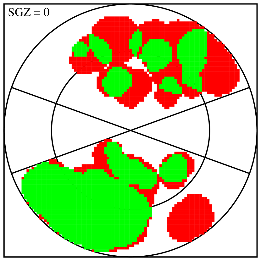
Figure 3: Overall overlap measure of ORSd and IRAS voids in the supergalactic plane $Z_{\mathrm{SG}}=0$. Green marks overlap, red marks no overlap. The overlap score in this slice is $\eta=0.43$.

6 Discussion

The two void images are similar, although the two galaxy samples are quite different. In Fig. 2 we present two sets of slices covering the supergalactic plane and slices immediately above and below it, all together spanning $-15<Z_{\mathrm{SG}}<15$.

Beyond the visual impression, we quantify the spatial similarity between the two void populations by deriving $\eta$, the ratio between the overlapping volume of the two void distributions and their union:

$$\eta=\frac{V_{1}\cap V_{2}}{V_{1}\cup V_{2}}$$ (7)

where $V_{1}$ represents the volumes occupied by voids in one distribution, and $V_{2}$ is the same quantity for the other distribution. In case of exact overlap we have $\eta=1$; for two random distributions the expected overlapping volume is simply $f_{1}f_{2}$, the product of the two void filling factors. E.g., if $f_{1}=f_{2}=0.5$ the expected score for a pair of random samples is $\eta=1/3$. On the other hand, if 80 per cent of the volumes overlap we would get $\eta=2/3$. See Fig. 3 for an illustration of the void overlap in the supergalactic plane.

Serendipitously, the details for our case happen to be quite similar to the above example: $f_{\mathrm{ORSd}}=0.54$ and $f_{\it IRAS}=0.48$. The overlap score is $\eta_{{\mathrm{ORSd-}{\it IRAS}}}=0.58$. In contrast, for random ORSd- and IRAS-like samples where half of the random IRAS locations are used in the random ORSd distributions we get $\eta_{\mathrm{rnd0.5}}=0.19\pm 0.04$; for completely unmatched sample pairs the score is $\eta_{\mathrm{rnd}}=0.13\pm 0.02$. The theoretical expectation for $\eta_{\mathrm{rnd}}$, based on the filling factors of the random samples, is $0.10\pm 0.02$, and the small actual excess over it is likely due to the geometrical constraints of the sample.

The above test measures the overall correlation between two void distributions without trying to match individual voids. As we identified (by eye) the corresponding voids in the two surveys (Table 2, column 10), we can also measure how well do the individual voids overlap. We do this by deriving $\eta$ values for a void from one of the samples and its counterpart(s) in the other sample. We report $\eta$ values for the ORSd–IRAS pairs in Table 2, column (11). The average value is $\bar{\eta}=0.47$. We can also give this score a more intuitive interpretation, by converting it to $d_{\mathrm{misfit}}(\eta)$, the distance (in fractions of a diameter units) at which one would need to place two identical spheres in order to get a specific value of $\eta$. Hence if there is exact overlap $\eta=1$ and $d=0$. If there is no overlap $\eta=0$ and $d>1$. A good reference point is at $d=0.5$ (two identical spheres misplaced by one radius), for which $\eta=5/27$. The average result we got for the ORSd–IRAS pairs corresponds to $d_{\mathrm{misfit}}(\bar{\eta})=0.25$.

Note that difference in void volumes is a contributing factor in the derivation of the (mis)fit scores. E.g., for two spheres at the same center but with one radius being $0.57$ of the other we would get the same $\eta$ as for identical spheres one radius apart. As on average the ORSd voids are somewhat bigger than the IRAS voids, we can quantify the contribution of this factor to the misfit score: it translates to a base misfit value of $d_{\mathrm{misfit(volume)}}\approx 0.1$.

In addition to the spatial correlation, the two distributions are also similar with regard to the average void properties – the total void filling factor, the average void diameter $\bar{d}_{\mathrm{void}}$ and the average void underdensity $\bar{\delta}$ (see Table 3). We find the later similarity to be of special interest: estimates of the relative bias between optical and IRAS samples based on the distribution of galaxies find $(b_{\mathrm{opt}}/b_{\it IRAS})^{\mathrm{gal}}\approx 1.5$ [Lahav, Nemiroff & Piran 1990, Baker et al. 1998]. However, as the galaxy underdensity in the voids in both surveys is $\bar{\delta}\approx-0.9$, the void finder analysis shows that on average there is practically no biasing in the voids: $(b_{\mathrm{opt}}/b_{\it IRAS})^{\mathrm{void}}=1$.

The only other work we are aware of which compared optical and IRAS galaxies in voids examined the Boötes void [Dey, Strauss & Huchra 1990]. There it was found that the density contrast of IRAS galaxies within the Boötes sphere is roughly equal to the (optical) upper limit for that region [Kirshner et al. 1987]. In this work we examine a distribution of voids, and use many more galaxies ($\approx 100$, compared to 12 IRAS galaxies in the Boötes); still, our result of little – or no – biasing between optical and IRAS galaxies in the voids is consistent with the Boötes result.

7 Summary

In this paper we present a comparison between two void distributions. These distributions sample the same volume of space, but were derived using the void finder code from two different galaxy samples – chosen optically (ORSd) and by the IRAS. The 9 significant voids we find in the ORSd match very well the locations of their IRAS counterparts, and our overlap/union ($\eta$) test shows a correlation significantly in excess of random. Combined with our previous analysis of the SSRS2s sample, we now have 3 different void catalogues all showing similar void properties, including the filling factor, average equivalent diameter and underdensity.

In all our samples so far voids are limited by the boundaries of the surveys – in this paper, by the ZOA and the limited depth ($80h^{-1}\mbox{Mpc}$); and in the SSRS2s by the narrow declination span (37$\aas@@fstack{\circ}$5). In order to overcome this limitation we intend to further extend our void catalogues using deeper (LCRS – Shectman et al. 1996) and wider (CfA2s – Huchra, Vogeley & Geller 1999) samples.

The fact that we find practically no biasing in the voids $(b_{\mathrm{opt}}/b_{\it IRAS})^{\mathrm{void}}=1$ indicates that voids may be a relatively bias-free environment. As such, they comprise an attractive target with which one can examine different cosmological models, and we intend to explore this possibility using $N$-body simulations.

Acknowledgments. We are indebted to Basilio Santiago for his help in unraveling the mysteries of the ORS. We thank Ofer Lahav, Myron Lecar, David Meiri and Sune Hermit for helpful discussions and comments. HE was supported by a Smithsonian Predoctoral Fellowship.

References

- [Baker et al. 1998] Baker J. E., Davis M., Strauss M. A., Lahav O., Santiago B. X., 1998, ApJ, 508, 6
- [Burstein & Heiles 1982] Burstein D., Heiles C., 1982, AJ, 87, 1165
- [da Costa et al. 1988] da Costa L. N., et al., 1988, ApJ, 327, 544
- [da Costa et al. 1998] da Costa L. N., et al., 1998, AJ, 116, 1
- [de Lapparent, Geller & Huchra 1986] de Lapparent V., Geller M. J., Huchra J. P., 1986, ApJ, 302, L1
- [Dey, Strauss & Huchra 1990] Dey A., Strauss M. A., Huchra J., 1990, AJ, 99, 463
- [El-Ad, Piran & da Costa 1997] El-Ad H., Piran T., da Costa L. N., 1997, MNRAS, 287, 790
- [El-Ad & Piran 1997] El-Ad H., Piran T., 1997, ApJ, 491, 421
- [Fisher et al. 1995] Fisher K. B., Huchra J. P., Strauss M. A., Davis M., Yahil A., Schlegel D., 1995, ApJS, 100, 69
- [Hermit et al. 1996] Hermit S., Santiago B. X., Lahav O., Strauss M. A., Davis M., Dressler A., Huchra J. P., 1996, MNRAS, 283, 709
- [Huchra, Vogeley & Geller 1999] Huchra J. P., Vogeley M. S., Geller M. J., 1999, ApJS, 121, 287
- [Kirshner et al. 1987] Kirshner R. P., Oemler A. Jr., Schechter P. L., Shectman S. A., 1987, ApJ, 314, 493
- [Lahav, Nemiroff & Piran 1990] Lahav O., Nemiroff R. J., Piran T., 1990, ApJ, 350, 119
- [Santiago et al. 1995] Santiago B. X., Strauss M. A., Lahav O., Davis M., Dressler A., Huchra J. P., 1995, ApJ, 446, 457
- [Santiago et al. 1996] Santiago B. X., Strauss M. A., Lahav O., Davis M., Dressler A., Huchra J. P., 1996, ApJ, 461, 38
- [Santiago 1998] Santiago B. X., 1998, private communication
- [Strauss et al. 1992] Strauss M. A., Davis M., Yahil A., Huchra J. P., 1992, ApJ, 385, 421
- [Saunders et al. 1991] Saunders W., et al., 1991, Nature, 349, 32
- [Saunders et al. 1998] Saunders W., et al., 1998, in Proc. of the XXXII Moriond Astrophysics Meeting, in press
- [Shectman et al. 1996] Shectman S. A., Landy S. D., Oemler A., Tucker D. L., Lin H., Kirshner R. P., Schechter P. L., 1996, ApJ, 470, 172
- [Strauss & Willick 1995] Strauss M. A., Willick J. A., 1995, Phys. Rep., 261, 271
- [Tully 1986] Tully R. B., 1986, ApJ, 303, 25
- [Tully 1987] Tully R. B., 1987, Nearby Galaxies Atlas. Cambridge University Press, Cambridge
- [Yahil et al. 1991] Yahil A., Strauss M. A., Davis M., Huchra J. P., 1991, ApJ, 372, 380