Air Showers and Geomagnetic Field.

Abstract

The influence of the geomagnetic field on the development of air showers is studied. The well known International Geomagnetic Reference Field was included in the AIRES air shower simulation program as an auxiliary tool to allow calculating very accurate estimations of the geomagnetic field given the geographic coordinates, altitude above sea level and date of a given event. Our simulations indicate that the geomagnetic deflections alter significantly some shower observables like, for example, the lateral distribution of muons in the case of events with large zenith angles (larger than 75 degrees). On the other hand, such alterations seem not to be important for smaller zenith angles. Global observables like total numbers of particles or longitudinal development parameters do not present appreciable dependences on the geomagnetic deflections for all the cases that where studied.

96.40.Pq, 13.10.+q, 02.70.Lq

I Introduction

The understanding of the origin and nature of high energy cosmic rays is one of the most challenging topics in contemporary astrophysics. With the knowledge currently available we cannot discard the possibility that the highest energy primary particles (those with energies above $10^{19}$ eV) have an entirely different origin than lower energy cosmic rays. This generates a variety of questions that cannot be definitively solved without adequate sets of experimental data. For this reason, several projects have been envisioned to determine the main characteristics of such cosmic rays.

The AUGER Observatory is one of these projects [1]. It consists in two identical hybrid detectors, respectively located in the Northern and Southern Hemisphere to get full sky coverage. Each hybrid detector consists in a surface array and a fluorescence detector, optimized to measure different parameters of the particle air showers generated after the incidence of high energy cosmic rays into the Earth’s atmosphere. The Observatory will be able to measure the arrival direction of the primary particle and the electromagnetic and muonic components of the showers at ground level. The longitudinal profile of the shower (number of charged particles as a function of the altitude) will be also available for approximately 10 % of the measured events. These special events are referred as “hybrid events”.

To clearly understand the relationship between the characteristics of the primary particle (energy, mass, etc.) and the quantities that will be measured by the AUGER detectors, it is essential to study the shower development by means of computer Monte Carlo simulations. We started working in this subject some years ago, and we have developed a set of programs to simulate air showers and manage all associated output data. Such simulating system is identified with the name AIRES (AIRshower Extended Simulations) [2, 3, 4].

The first version of AIRES was developed on the basis of the well known MOCCA program, created by A. M. Hillas for the Haverah Park experiment [5]. The AIRES program incorporates substantial improvements, in particular from the computational point of view. Later versions do also include additional physics algorithms that complement the original set of procedures taken from MOCCA.

The particles currently processed by AIRES are: gamma rays, electrons and positrons, muons, pions, kaons, nucleons, anti-nucleons and nuclei. Neutrinos are generated (in pion or muon decays, for example) and accounted for their energy, but not tracked. The shower particles can undergo the following processes: $(1)$ Electromagnetic interactions: Pair production, bremsstrahlung (electrons and positrons), Compton and photoelectric effects and emission of knock-on electrons ($\delta$ rays). The LPM effect and dielectric suppression that affect high energy production and bremsstrahlung processes are taken into account using recently developed procedures (for details see reference [4]). $(2)$ Hadronic interactions: Nuclear fragmentation and inelastic collisions, managed via calls to external packages like SIBYLL [6] or QGSJET [7]. $(3)$ Unstable particle decays. $(4)$ Particle propagation includes continuous energy losses (ionization) and scattering. The curvature of the Earth is always taken into account (it is possible to process showers with zenith angles in the full range [$0^{\circ}$, $90^{\circ}$]), as well as geomagnetic deflections.

The purpose of this work is to analyze the effect of the Geomagnetic Field (GF) on the development of the showers, giving quantitative estimates of the influence of the GF on the very high energy showers using environmental conditions similar to the ones of the AUGER observatory.

We have first studied the principal characteristics of the GF: Its origin, magnitude and variations. Thereafter we have analyzed the different GF models that are normally used: The dipolar models [8] which consider the GF as generated by magnetic dipoles; and the so-called International Geomagnetic Reference Field (IGRF) [9], a more elaborated model, based on a high-order harmonic expansion whose coefficients are fitted with data coming from a network of geomagnetic observatories all around the world.

One of the conclusions that comes out from our analysis is that the dipolar models are not useful to evaluate the GF at a given arbitrary location with enough accuracy. On the other hand, the predictions of the IGRF proved to match with the corresponding experimental data with errors that are at most a few percent. For example, the difference between the IGRF predictions on the field components and the experimental data are less than 500 nT (nanotesla, 1 ${\rm nT}=10^{4}$ gauss). We have therefore selected the IGRF to link it to the simulation program AIRES, as an adequate model to synthesize the GF at a given geographical location and time.

This paper is organized as follows: In section 2 we report on the simulations performed to analyze the influence of the GF on the shower development and in section 3 we place our final remarks and conclusions. In appendix A we give a short description of the GF and we briefly comment different models that exist at present and discuss the practical implementation of the GF in the AIRES program. Additional information needed to analyze the influence of the GF without other distortions, like the ones introduced by the geometry (the axis of the showers are usually inclined) and the attenuation in the atmosphere, is given in appendix B.

II Simulations

We have analyzed the influence of the GF on air shower observables performing some simulations in a variety of initial conditions.

We have simulated several thousands of showers with varying primary energy (in the range of ultra-high energies) and zenith angle. We have considered different sites in our simulations, which imply different intensities and directions of the GF. In most cases these environmental conditions correspond to the Northern and Southern sites for the AUGER observatory, which are, respectively Millard County (Utah, USA) and El Nihuil (Mendoza, Argentina) [1].

It is interesting to note that the average GF intensity at the Millard site is twice the corresponding one for the El Nihuil Southern site (50000 nT and 25000 nT, respectively). As a consequence, the influence of the field on the particles’ paths will be different at each site, being more appreciable at Millard where the GF is more intense.

Our analysis is mainly based on comparisons of average values of observables coming from simulations performed with the program AIRES alternatively taking and not taking into account the GF deflections of charged particles (For a more detailed description of the implementation of the GF in AIRES, see appendix A).

The direct inspection of global observables such as the longitudinal development of all charged particles (total number of charged particles plotted against the atmospheric depth, $X$), shower maximum (atmospheric depth where the total number of charged particles is maximum), total number of particles at ground, etc,  shows no evident effect of the GF.

To illustrate this point we have plotted in figure 1 the longitudinal development of the number of all charged particles and muons for showers initiated by $10^{20}$ eV gammas (a) and protons (b). The zenith angle is $81.5^{\circ}$ ($\cos\Theta=0.15$), the azimuth is fixed at $90^{\circ}$ to ensure a strong effect of the GF, and the environmental conditions are those of Millard site. Comparing the plots coming from the simulations with (solid line) and without (dashed line) GF, it is evident that there are no significant differences due to the GF deflections for both charged particles and muons cases. One of the main implications that can be derived from these figure is that the GF does not induce any appreciable variations in both the position of the maximum ($X_{max}$) and the maximum number of charged particles ($N_{max}$). We recall that these observables are the main quantities that can be measured with the fluorescence detector, and are essential for determining the shower energy and primary composition.

Although the differences between the simulations taking and not taking into account the GF are not significant for global observables, as we have shown before, some variations do appear when a detailed analysis of some particle distributions is made. This is the case, for example, of the density distribution of muons at ground level (lateral distribution of muons).

This kind of particles is the most affected by the GF. This is due to the fact that muons usually travel long distances without interacting with the medium, allowing for bigger GF deflection angles. Additionally, for large zenith angles, the muonic component of the shower generally represents an important fraction of the measurable ground level signal. Therefore this case should be studied in detail in order to establish whether or not the standard ground measurement techniques [1] (developed for nearly vertical showers) are valid when the zenith angle not small.

The plots in figure 1 illustrate how the muonic component of the showers becomes progressively more important (in comparison with all the charged particles) as long as the shower continues its evolution after having reached its maximum.

The ratio between the numbers of muons and electromagnetic particles, that is,

$$\eta=\frac{\hbox{Number of }\mu^{+/-}}{\hbox{Number of }\gamma+\hbox{Number of }e^{+/-}}$$ (1)

gives a convenient quantitative measure of the relative importance of the muonic component in a determined case.

In figure 2, the ratio $\eta$, evaluated at ground level, is plotted versus the zenith angle for the typical case of $3\times 10^{20}$ eV proton showers. The ground level altitude is 1400 m.a.s.l.  $\eta$ is practically constant for zenith angles lower than 60 degrees. Around this point $\eta$ begins to rise abruptly (the parameter grows more than 2 orders of magnitude when the zenith angle passes from 50 to 70 degrees) and reaches a maximum at approximately 75 degrees. $\eta(70^{\circ})$ is some 400 times larger than $\eta(0^{\circ})$. Beyond that point $\eta$ decreases slightly.

There is another remarkable experimental reason to study the influence of the GF on the lateral distribution of muons for large zenith angles: The total average signal observed in the C̆erenkov detectors 1.2 m depth (as in the case of the Auger Observatory [1]) is dominated by the muonic component which is twice the signal of the electromagnetic particles for zenith angles of 80 degrees, that is, a fraction tree times larger than the corresponding one for a zenith of $30^{\circ}$.

In the remaining part of this section we are going to present some representative results obtained from the simulations performed with the AIRES program. We have analyzed a variety of initial conditions: Two geographical locations (El Nihuil and Millard sites) each one with different GF, zenith angles in a wide range, from $0^{\circ}$ to $81.5^{\circ}$, and ultra-high energies in the range $10^{19}$ eV to $10^{20.5}$ eV. For very inclined showers the effect of the GF deflections on the lateral distribution of muons is very significant. This can be put into evidence comparing figures 3 and 4. These figures corresponds to $10^{20}$ eV gamma showers and the injection altitude is the top of the atmosphere. In these plots, the muon density is represented at each case by means of diagrams and contour line plots. The plots labelled (a) represent the row ground densities, while the plots labelled (b) and (c) represents the geometrical (equation (B3)) and geometrical with attenuation correction (equation (B11)) projections onto the shower front plane, respectively. The plots of figure 4 (GF turned off) show that the well known distortion that makes contour lines approximately elliptical can be eliminated after applying the procedures of appendix B: The contour lines of figure 4 c are approximately circles, concentric with the shower axis. The contour lines of figure 4 b, are also approximately circular, but a careful analysis shows that they are slightly eccentric (in this figure the centers are shifted towards the right). This typical eccentricity indicates that the attenuation correction (equation (B11)) cannot be neglected.

When the GF is taken into account (figure 3), the two dimensional density pattern is different, and the application of the procedures to project onto the shower front plane permits putting in clear evidence the lack of cylindrical symmetry of the shower in this case.

Ground and shower front plane (with all corrections) $\mu^{+}$ and $\mu^{-}$ distributions are presented in figures 5 and 6, in the same conditions as in figure 3 and 4, but for proton showers and injection altitude of 200 g/cm², respectively taking and not taking into account the GF. In this case the injection altitude is 200 g/cm² in order to have enough signal at ground level. In the case of gamma showers, we have chosen the injection altitude at the top of the atmosphere because this kind of particles are very penetrating ones due to the LPM effect [4]. The direction of the horizontal field (H) and the projection of the GF onto the shower front plane are indicated for convenience. When the GF is enabled (figure 5) the separation between $\mu^{+}$ and $\mu^{-}$ becomes evident.

The simulations corresponding to the distributions of figures 3 and 5 were performed for very inclined showers (zenith angle $81.5^{\circ}$), and a relatively intense GF (${\rm F}=52800$ nT). In the case of El Nihuil site, where the GF intensity is about one half of the previous one, the effect of the GF deflections is smaller, but not negligible.

The distortions generated by the GF for very inclined showers diminish dramatically as long as the zenith angle is reduced. To illustrate this point, let us consider the plots of figure 7, which corresponds to $3\times 10^{19}$ eV proton showers with zenith angle $60^{\circ}$. A careful inspection of these graphs permits detecting some little differences between the $\mu^{+}$ and $\mu^{-}$ distributions. Such differences, however, compensate noticeably when evaluating the total ($\mu^{+}$ and $\mu^{-}$) distribution (not plotted here), which is practically equivalent to the corresponding one coming from the simulations without GF.

III Conclusions

We have discussed in this work the influence of the geomagnetic field on the most common observables that characterize the air showers initiated by astroparticles. The data used in our analysis were obtained from computer simulations performed with the AIRES program.

Our work includes the analysis of the main properties of the geomagnetic field, as well as the implementation of the related algorithms in the program AIRES.

By means of the International Geomagnetic Reference Field (IGRF) it is possible to make accurate evaluations of the average geomagnetic field at a certain place given its geographical coordinates, altitude above sea level and time. We have used this tool to run the simulations using a realistic geomagnetic field.

The changes that global observables like the longitudinal development of all charged particles experiment when the geomagnetic field is taken into account, are generally small. On the other hand, we have found that in some distributions, like in the lateral distribution of muons, for the case of realistic fields and for large zenith angles (larger than 70 degrees), the differences between the cases where such field is taken or not taken into account become significant.

For showers with zenith angles less than 70 degrees, the deflections due to the GF do not generate important alterations in such distributions, allowing for safe application of analysis techniques that do not take care of the effect of the GF deflections.

It is worthwhile to mention that this work is restricted to the study of the consequences derived from the deflections of charged particles that move under the influence of the Earth’s magnetic field. Other effects modifying the behavior of air showers and related to the GF will be considered in future works.

A Geomagnetic deflections of charged particles

1 Calculating the Earth’s magnetic field

The Earth’s magnetic field is described by seven parameters [8], namely, total intensity (F), inclination (I), declination (D), horizontal intensity (H), vertical intensity (Z), and the north (X) and east (Y) components of the horizontal intensity. D is the angle between the horizontal component of the magnetic field and the direction of the geographical north and I is the angle between the horizontal plane and the total magnetic field. It is considered positive when the magnetic field points downwards. Also Z is positive when I is positive [8].

The GF is generated by internal and external sources. The first ones are related to processes in the interior of the Earth’s core and the intensity of the field generated goes from 20000 to 70000 nT while the second ones would be related to ionized currents in the high atmosphere and it contribution is around 100 nT [8].

The different components of the GF (external and internal) are not uniform over position and time. The secular and periodic variations [8] are originated by the external field. The firsts go from 10 up to 150 nT per year and the second ones are less than 100 nT. Also, there are sudden disturbances in the GF (namely, magnetic storms) which may last from hours up to several days and rarely modify the field in more than 500 nT.

The simplest way to model the GF is to assume that it is generated by a magnetic dipole (dipolar central and eccentric models) [8]. However, when a more accurate reproduction of the field is needed, it is necessary to go beyond the dipole approximation and make a higher order harmonic analysis of the GF [8]. Due to the spherical symmetry of the problem, the solution can be conveniently expressed in terms of the following expansion

$$\phi=a\sum_{n=1}^{N}\sum_{m=0}^{n}\left(\frac{a}{r}\right)^{n+1}[g_{nm}\cos m\lambda+h_{nm}\sin m\lambda]P_{n}^{m}(\cos\varphi)$$ (A1)

where $a$ is the mean radius of the Earth (6371.2 km), $r$ is the radial distance from the center of the Earth, $\lambda$ is the longitude eastwards from Greenwich, $\varphi$ is the geocentric colatitude, and $P_{n}^{m}(\cos\varphi)$ is the associated Legendre function of degree $n$ and order $m$, normalized according to the convention of Schmidt. $N$ is the maximum spherical harmonic degree of the expansion. The International Geomagnetic Reference Field (IGRF) [9] is a series expansion like (A1) where the coefficients are adjusted to fit experimental measurements coming from a network of geomagnetic observatories located all around the world. Set of spherical harmonic coefficients ($g_{nm}$ and $h_{nm},N=10)$ at 5-year intervals starting from 1900 are currently available. Coefficients for dates between 5-year epochs are obtained by linear interpolation between the corresponding coefficients for the neighboring intervals. The error of the field components and the D and I angles are less than 500 nT and 30 arc minutes, respectively. These errors are relatively small and this makes the IGRF model a very useful tool to estimate the GF at any geographic location and any time belonging to its validity interval.

We have evaluated the results coming from the different models already mentioned in a variety of situations, in order to establish which of them is the most convenient to cover the needs arising in an air shower simulation algorithm. Our conclusion is that the IGRF is the most convenient model that can give accurate estimations of the GF to be used in air-shower simulations [10]. An illustrative example is placed in figure 8, where a comparison between experimental data [11] and the IGRF model is plotted versus time. The F, H and Z components are shown. In all cases, the absolute difference between estimated and measured fields is always less than 200 nT. The errors in the estimation of I and D (not displayed) are always less than 0.5 degrees. More illustrative examples of the different models of the GF are plotted in reference [10].

2 Practical Implementation

It is assumed that the shower develops under the influence of a constant and homogeneous magnetic field which is evaluated before starting the simulations . In order to calculate the GF, special subroutines using the IGRF model have been incorporated to the AIRES program [2].

If a charged particle $q$ advances a distance $\Delta s$ in a uniform, static magnetic field $\mathbf{B}$ ($\Delta s=\beta c\Delta t$, $\beta=v/c$), the motion can be approximately calculated via :

$$\widehat{\mathbf{u}}(t+\Delta t)\cong\widehat{\mathbf{u}}(t)+\frac{d\widehat{\mathbf{u}}}{dt}\Delta t=\widehat{\mathbf{u}}(t)+\left(\frac{qc^{2}\Delta t}{E}\right)\widehat{\mathbf{u}}\times\mathbf{B}$$ (A2)

where $\widehat{\mathbf{u}}=\frac{\mathbf{v}}{\mathbf{\left|v\right|}}$ is the unit velocity vector, $\mathbf{v}$ is the velocity of the particle, $E$ is the total energy of the particle (rest plus kinetic) and $c$ is the speed of light.

For this approximation to be valid, it is needed that

$$\omega\Delta t=\frac{\omega\Delta s}{\beta}\ll 1$$ (A3)

where

$$\omega=\frac{qc^{2}B}{E}$$ (A4)

is the angular velocity of the particle [12].

The magnetic deflection algorithm implemented in AIRES makes use of equation (A2) (taking care that (A3) is always satisfied) to evaluate the updated direction of motion at time $t+\Delta t$. However, it also uses a “technical trick”, inspired in a similar procedure used in the well-known program MOCCA [5]: The path $\Delta s$ is divided in two halves of length $\Delta s/2$ each. Then the particle is moved the first half using the old direction of motion $\widehat{\mathbf{u}}(t)$, and the second one with the updated vector $\widehat{\mathbf{u}}(t+\Delta t).$

B Geometry and Attenuation in the atmosphere

To analyze adequately the modifications introduced by the GF deflections in the shower observables, it is convenient to subtract the deviation introduced geometrically (due to the fact that the shower axes are usually inclined) and related to the atmospheric attenuation. In figure (9), the basic geometrical elements corresponding to an inclined shower are represented schematically. Let $\Theta$ and $\Phi$ be the shower zenith and azimuth angles, respectively. If $(r,\varphi)$ are the polar coordinates of P in the ground plane and $(r_{0},\beta)$ represent the polar coordinates of the same point with respect to the shower front plane (plane perpendicular to the shower axis containing P), it is easy to show that

$$r_{0}=\overline{{\bf PQ}}=r\,\sqrt{1-\sin^{2}\Theta\cos^{2}(\varphi-\Phi)}$$ (B1)

and

$$\tan\beta=\frac{\tan(\varphi-\Phi)}{\cos\Theta}$$ (B2)

In general, the density of a given type of particles (for example muons) at ground level will be a function of $r$ and $\varphi$, $\rho_{g}(r,\varphi)$. On the oder hand, showers that develop with no GF deflections will have cylindrical geometry with respect to the shower axis and the density measured on the shower front plane will not depend on $\beta$: $\rho_{0}(r_{0},\beta)$=$\rho_{0}(r_{0})$. For vertical showers, $\rho_{0}$ and $\rho_{g}$ refer to the same magnitude, but when the zenith angle is not zero, $\rho_{0}$ is different from $\rho_{g}$.

If the variation on the total number of particles with the atmospheric depth is neglected, then $\rho_{0}$ and $\rho_{g}$ are related by a simple geometrical transformation:

$$\rho_{0}(r_{0},\beta)=\frac{\rho_{g}(r,\varphi)}{\cos\Theta}$$ (B3)

(in this formula, $\rho_{0}$ will not depend on $\beta$ for cylindrically symmetrical showers). It is well known, however, that the number of shower particles is not constant for different depths. This means that the density $\rho_{0}$ depends on $X$, the depth of point Q, and therefore equation (B3) will not be approximate enough in these cases.

A transformation between $\rho_{0}$ and $\rho_{g}$ that proves to work acceptably well in most practical cases can be easily derived accepting the following empirical parameterization for the lateral distribution at varying atmospheric depth [1]

$$\rho(r_{0},X)=k(X)\,r_{0}^{\eta(X)}\,f_{0}(r_{0})$$ (B4)

where $k$ and $\eta$ are functions of $X$, and $f_{0}$ only depends on $r_{0}$.

Let $X_{g}$ be the vertical depth of the ground plane. The vertical depth at point Q, $X$ is usually not much different from $X_{g}$, and can be excellently approximated by means of a locally isothermic atmosphere:

$$X\simeq X_{g}e^{-\xi z_{Q}}$$ (B5)

where $\xi$ is a parameter characterizing the atmosphere which can be determined easily, and

$$\quad z_{Q}=\frac{r}{2}\sin(2\Theta)\cos(\varphi-\Phi)$$ (B6)

is the altitude of point Q (with respect to the ground level)

From equation (B4) it is easy to show that

$$\frac{\rho_{0}(r_{0},X)}{\rho_{0}(r_{0},X_{g})}=\frac{k(X)}{k(X_{g})}\,r_{0}^{[\eta(X)-\eta(X_{g})]}$$ (B7)

When $X$ $>$ $X_{\rm max}$ the shower is in its attenuation phase, and $k(X)$ (related to the total number of particles at depth $X$) can be approximated as ($X\simeq X_{g}$):

$$\frac{k(X)}{k(X_{g})}\simeq e^{-a(X-X_{g})}$$ (B8)

In the same conditions, $\eta(X)$ can be satisfactorily represented as a linear function of $X$

$$\eta(X)-\eta(X_{g})\simeq b(X-X_{g})$$ (B9)

$a$ and $b$ are parameters to be determined. Notice that $a$ and $b$ do not depend on $r_{0}$. Equations (B7), (B8) and (B9) yield

$$\rho_{0}(r_{0},X)=\rho_{0}(r_{0},X_{g})\exp\left[-(a-b\ln r_{0})(X-X_{g})\right]$$ (B10)

Using equation (B3) and calling $\rho_{0}(r_{0},X_{g})$=$\rho_{0}(r_{0})$ (assuming cylindrical symmetry with respect to the shower axis), we can write

$$\rho_{g}(r,\varphi)=\cos\Theta\rho_{0}(r_{0})\exp\left[-(a-b\ln r_{0})(X-X_{g})\right]$$ (B11)

The dependence of the right hand side of this equation on $r$ and $\varphi$ derives from equations (B1), (B5) and (B6).

In our analysis, the free parameters $a$ and $b$ of equation (B11) were always evaluated performing least squares fits to data coming from simulations with the GF disabled (this ensures the cylindrical symmetry of the shower front plane distributions). The associated simulations performed in similar conditions, but enabling the GF were processed using the same $a$ and $b$ obtained from the “no GF” case. This procedure ensures then that the average effect of geometry and attenuation is properly subtracted, and that the lack of cylindrical symmetry observed in the corresponding cases is direct consequence of the GF deflections.

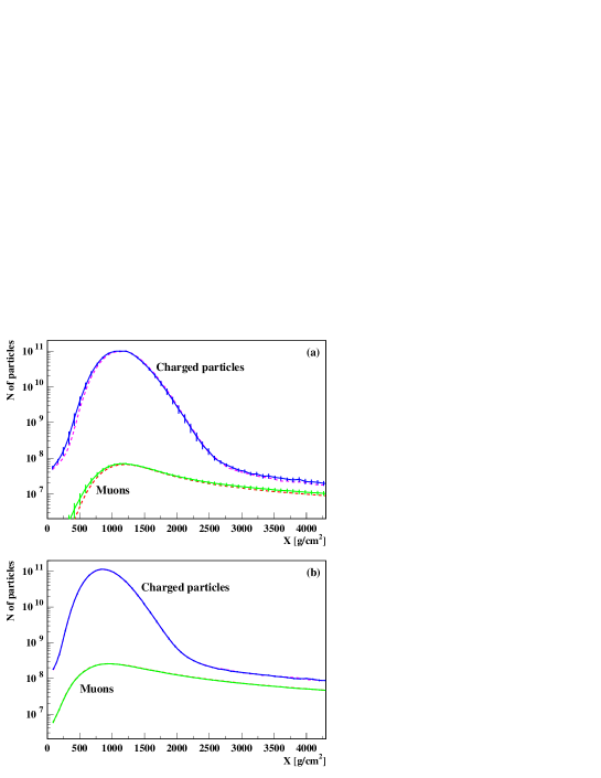
FIG. 1.: Longitudinal development of all charged particles and muons, for $10^{20}$ eV gamma (a) and proton (b) showers. The solid (dashed) lines correspond to the case of GF enabled (disabled). The abscissas represent the slant path along the shower axis, measured from the injection point. The errors bars correspond to two times the RMS error of the mean.

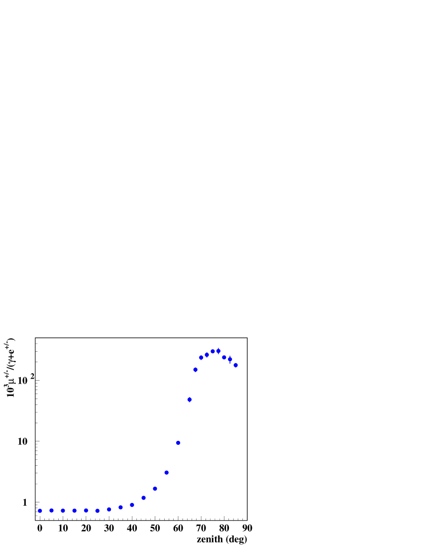
FIG. 2.: The ratio $\eta$ versus the zenith angle. The simulations correspond to $3\times 10^{20}$ proton showers. Site: El Nihuil.

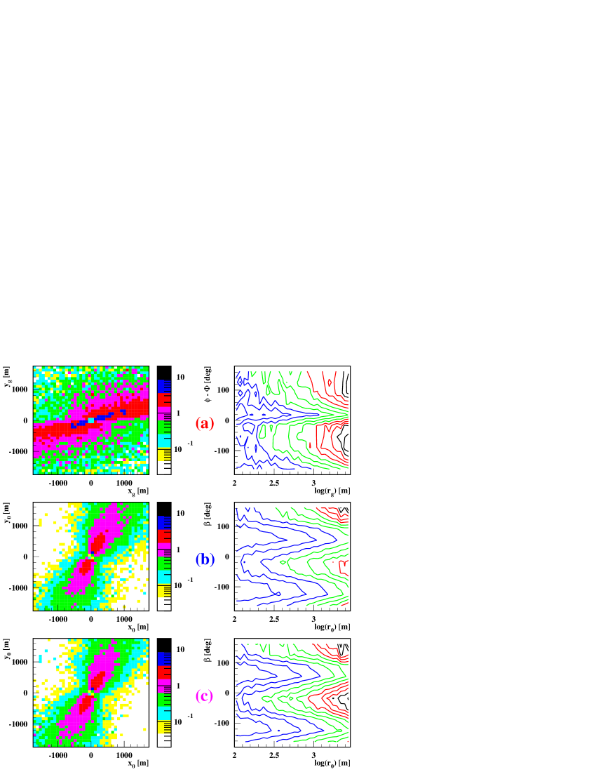
FIG. 3.: Two dimension lateral distribution of muons for $10^{20}$ eV gamma showers, zenith angle $81.5^{\circ}$ at Millard site. Injection at the top of the atmosphere. The distributions are represented as false color diagrams (left column) and contour plots (right column). (a) Row distribution at ground. (b) Geometrical projection onto the shower plane (equation (B3)). (c) Geometrical projection plus attenuation correction (equation (B11)).

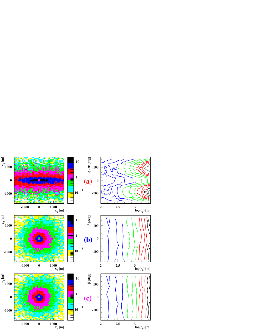
FIG. 4.: Same as figure 3, but with the GF disabled.

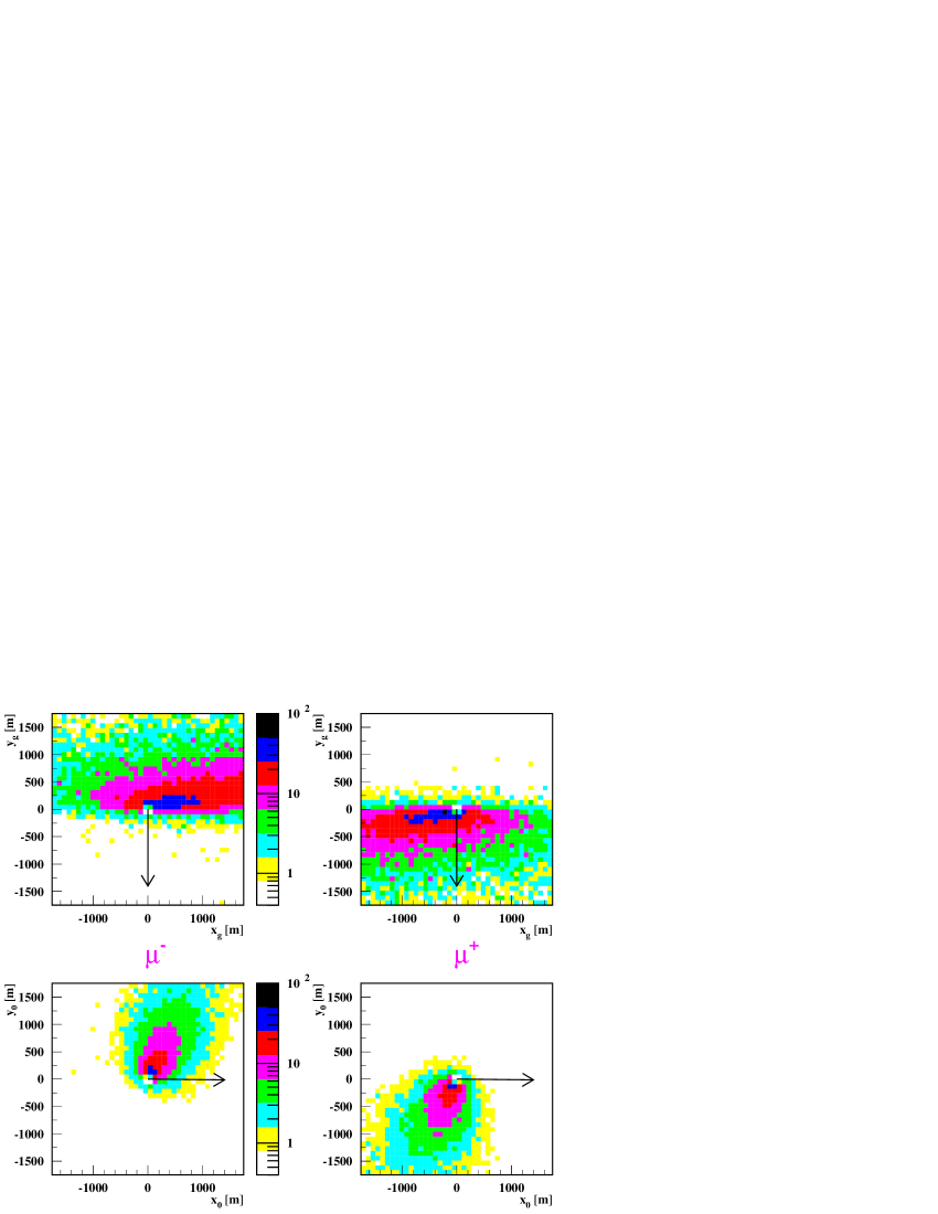
FIG. 5.: False color representations of the two dimension $\mu^{+}$ and $\mu^{-}$ density distribution. The upper plots correspond to the row ground plane distributions, while the lower ones to the corrected shower front plane distributions (equation (B11)). The arrows indicate the direction of the H component of the GF (upper plots) or the direction of the projection of the GF onto the shower front plane (lower plots). The conditions of the simulations are the same as in figure 3, but for proton showers and injection altitude 200 g/cm².

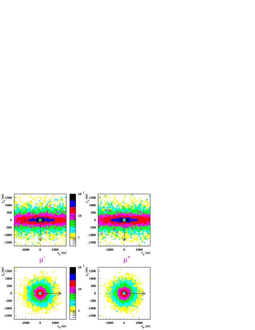
FIG. 6.: Same as figure 5, but with the GF disabled.

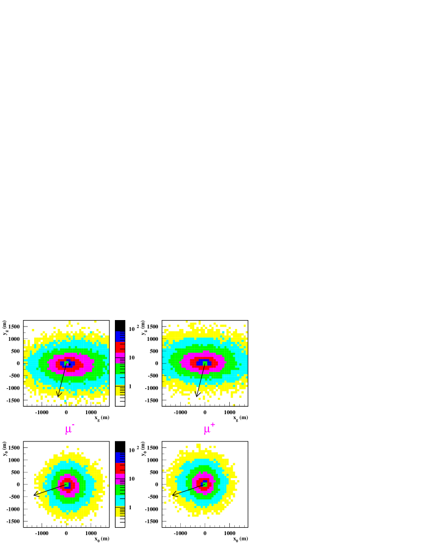
FIG. 7.: Same as figure 5 but for $3\times 10^{19}$ eV proton showers, $60^{\circ}$ zenith angle, site El Nihuil (GF enabled).

$$\begin{array}[]{cc}\hbox{\epsfbox{acaciaf.eps}}\\ \hbox{\epsfbox{acaciah.eps}}\\ \hbox{\epsfbox{acaciaz.eps}}\end{array}$$

FIG. 8.: Comparison between experimental data and the IGRF model. The absolute difference between the experimental and the IGRF prediction is always less than 200 nT.(Experimental data: Las Acacias observatory, Argentina).

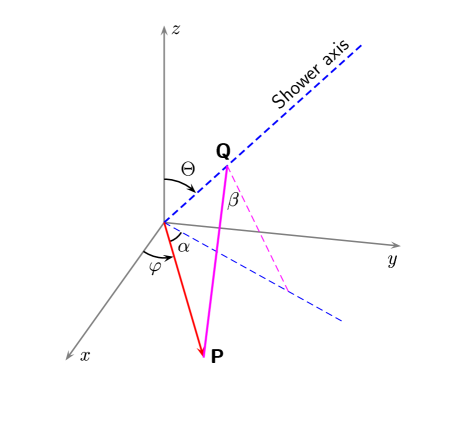
FIG. 9.: Schematic representation of the polar coordinates of the point P in the ground ($r$, $\varphi$) and shower front ($r_{0}$, $\beta$) planes. $\alpha=\varphi-\Phi$, where $\Phi$ is the shower azimuth angle.

REFERENCES

- [1] The Auger Collaboration The Pierre Auger Observatory. Design Report, 1997. Second Edition. This Report, the library of GAP Technical Notes and other information on the AUGER Project are available at the following Web page www.auger.org.
- [2] Sciutto S J 1999 AIRES, a system for air shower simulations. User’s manual and reference guide, version 2.0.0. The AIRES software and documentation are available electronically at the following Web address: www.fisica.unlp.edu.ar/auger/aires.
- [3] Anchordoqui L, Dova M T, Epele L N and Sciutto S J 1999, Phys. Rev. D 59 094003.
- [4] Cillis A N, Fanchiotti H, Garcia Canal C A and Sciutto S J 1999 Phys. Rev. D 59 113012.
- [5] Hillas A M 1997 Nucl. Phys. B (Proc. Suppl.) 52B 29; Hillas A M 1985 Proc. 19th ICRC (La Jolla) 1 155.
- [6] Fletcher R T, Gaisser T K, Lipari P and Stanev T 1994 Phys. Rev. D 50 5710; Engel J, Gaisser T K , Lipari P and Stanev T 1992 Phys. Rev. D 46 5013.
- [7] Kalmykov N N and Ostapchenko S S 1993 Yad. Fiz. 56 105; Phys. At. Nucl. 56 (3) 346; Kalmykov N N, Ostapchenko S S and Pavlov A I 1994 Bull. Russ. Acad. Sci. (Physics) 58 1966.
- [8] Chapman S and Bartels J 1940 Geomagnetism, Oxford University Press (Clarendon), London and New York, Volumes 1 and 2.
- [9] The data, software and documentation related with the International Geomagnetic Reference Field are distributed by the National Geophysical Data Center, Boulder (CO), USA, and can be obtained electronically at the following Web address: www.ngdc.noaa.gov.
- [10] Cillis A N and Sciutto S J 1997 Geomagnetic Field and Air Shower Simulations, preprint astro-ph/9712345.
- [11] Gianibelli J, Center of Geomagnetic Studies, La Plata University, private communication.
- [12] Jackson J D 1975 Classical Electrodynamics, John Wiley Sons, New York second edition.