Calibrating the Mixing Length Parameter for a Red Giant Envelope

Abstract

Two-dimensional hydrodynamical simulations were made to calibrate the mixing length parameter for modeling red giant’s convective envelope. As was briefly reported in Asida & Tuchman (1997), a comparison of simulations starting with models integrated with different values of the mixing length parameter, has been made. In this paper more results are presented, including tests of the spatial resolution and Large Eddy Simulation terms used by the numerical code. The consistent value of the mixing length parameter was found to be 1.4, for a red giant of mass $1.2M_{\sun}$, core mass of $0.96M_{\sun}$, luminosity of $200L_{\sun}$, and metallicity $Z=0.001$.

1 Introduction

Convection is a major process taking place in reg giant (RG) envelopes. In a previous letter (Asida & Tuchman (1997), hereafter AT97), results of a study of this subject were reported briefly. In the present paper, more results of this study are presented.

Throughout the paper, the reference one-dimensional (1D) model of convection is the mixing length theory (MLT, Bohm-Vitense (1958)), according to the prescription of Cox & Giuli (1968). Laboratory experiments, observations of the outer layers of the solar convective zone, and theoretical understanding have demonstrated that convection is much more complicated than MLT assumes.

Analysis of experiments of convection in a box, in which a temperature gradient was established by using Helium at about 5K and controlling the boundary conditions, have shown that convective flow is non-local with defined narrow streams going from the top down (and vice versa), i.e. the existence of a downstream at a given depth at a given time depends upon the existence of a downstream in a higher point at previous time and not upon local parameters only. This phenomenon is known as hard turbulence (see Helsot et al. (1987); Castaing et al. (1989); Wu & Libchaber (1992); Tligner et al. (1993)).

Observation of the outer layers of the sun have shown the existence of two dimensional cells of upstreams , in a variety of sizes and shapes, with the boundaries of these cells being the downstreams, i.e. the flow is not symmetric (see Nordlund & Stein (1995)).

During the years, many studies were made in order to overcome the simplifications of MLT. Several non-local and non-instantaneous theories were proposed (Spiegel (1963); Ulrich (1970, 1976); Stellingwerf (1982); Gehmeyr & Winkler (1992); Grossman & Narayan (1993); Grossman et al. (1993); Grossman (1996); Xiong et al. (1997); Canuto (1997); Canuto & Dubovikov (1998)). A common feature in these theories is using turbulence theory techniques in which the hydrodynamical quantities at each point are constructed of two components: a constant value and a varying value. Equations are formulated for each of the varying quantities which are then used to determine the convective velocity and flux. These equations include creation and diffusion terms and thus constitute a set of coupled partial difference equations. Maybe because of this complexity, there is no wide usage of these theories. Xiong et al. (1998a,b) have used one of these theories to compute linear pulsation times of RR Lyrae and Long Period Variables. Buchler et al. (1999) are using a simplified 1D model of turbulent energy diffusion and convection with eight free parameters to describe Cepheid and RR Lyrae variables.

Canuto & Mazzitelli (1991) used turbulence models to construct an alternative model for MLT which includes a full spectrum of eddy sizes (see also Canuto et al. (1996)). This model is still local and instantaneous, but is easy to include in astrophysical codes. It was found that this model yields higher values of convective flux than MLT at efficient convection regimes, and lower values of convective flux at inefficient convection regimes. This model was found to be preferable to MLT in many studies (see Canuto (1996); Canuto & Christensen (1998)). These studies included red giant evolution (Stothers & Chin (1995, 1997)), Heliosesmology (Basu & Antia (1994)) and calculations of uvby colors of A F and G stars (Smalley & Kupka (1997)). The superiority of this model, for example in modeling red giant evolution, was the usage of a constant parameter for various masses, while when using MLT there was a need to change the mixing length parameter with mass. However, Ludwig et al. (1999) have shown that a varying calibration is needed for this model too.

Alternatives to the usual mixing length used in MLT (which is a free parameter times the pressure scale height) were suggested. These included using the density scale height (Schwarzchild (1961)) and the distance from the boundary of the convection zone as in Canuto & Mazzitelli (1991).

For a correct modeling of red giant variables, the lack of time dependence and the locality of MLT are major disadvantages. The convection velocities, as predicted by MLT, and the radial velocities associated with pulsation are of the same order of magnitude (of $10\text@frac{km}{sec}$). Thus, interaction of the two phenomena is expected.

Ad hoc prescriptions were made in order to take into account time dependence in dynamical calculations with MLT (for example, pulsation calculation of Miras, see Tuchman (1980)). In these calculations, the convective flux at a given time is determined by using MLT and the flux at a previous time assuming a typical convective time scale estimated by convection velocity. In other calculations, like evolution of massive stars, a non locality is presented to MLT in particular when treating penetration (or overshoot) of convection to stable neighboring zones. A common assumption is that this overshoot region is proportional to the mixing length at the edge of the convection region. These methods are obviously not rigorous and not intended to describe these processes precisely (for example see Maeder & Conti (1994).

Being mainly a hydrodynamical phenomenon, an appealing method for modeling convection is by using numerical multidimensional simulations. In this approach, no explicit model of convection is needed, and thus no mixing length parameter is assumed. Time dependence and non locality are naturally present. However, convection is multidimensional and the flow has many length scales and time scales, that might be smaller by far than other typical scales of the problem. This is why such calculations are not suitable for all problems with convection.

Numerical simulations of the hard turbulence experiments mentioned above where made (Werne 1993,1994, Kerr (1996)). These calculations reproduced the typical narrow streams of the experiments, and revealed that the origin of the flow was the thin boundary layers at the bottom and at the top of the experimental box.

Many studies were made in order to understand general features of convective flow (Hurlburt et al. (1984); Chan & Sofia (1986); Malagoni et al. (1990); Cattaneo et al. (1990); Hossain & Mullan (1991); Cattaneo et al. (1991); Chan & Gigas (1992); Singh & Chan (1993); Rast and Toomre (1993); Xie & Toomre (1993); Porter & Woodward (1994)). Typically, these studies assumed simplified physical assumptions, such as ideal gas equation of state, constant opacity and constant gravitation. The systems were confined in a box with an initial unstable polytropic profile. Boundary conditions were periodic on the sides of the box, no flow was assumed in and out of the bottom and top of the box, a constant temperature gradient at the bottom and a constant temperature at the top. Some of the simulations assumed planar symmetry using 2D codes, while other used three-dimensional (3D) codes.

Summary of some the results of these studies is: there is an asymmetry in the flow with narrow rapid downstreams and wider upstreams and the 3D picture resembles the observations of the sun with cells of upstreams; the flow in the wider upstreams is somewhat more turbulent; the size of the cells increases with depth so downstreams merge. This picture is revealed when using high resolution, while low resolution simulations show laminar flow with big convection cells. The internal energy flux in the downstreams is relatively large, but a large kinetic energy flux with opposite sign almost cancels the net energy flux in the downstreams. Near the outer boundary, convection might be supersonic.

Other ”simulation in a box” studies were dealing with invoking of p-modes in the convection zone (Bogdan et al. (1993)), producing g-modes below (and above) the convection region (Hurlburt et al. (1986)) and penetration of convection to neighboring layers (Hurlburt et al. (1994) Singh et al. 1994,1995).

Attempts have been made to simulate the outer layers of the solar convection region (Stein & Nordlund 1989,1998, Kim et al. (1995)). Since the computation box in these simulations included only a fraction of the convection region, penetrative boundary conditions were applied at the bottom of the computation box. The outer layers which were included in the simulations and in which a superadiabatic gradient exist, are the most sensitive to the convection model. These simulations reproduced the granulation pattern of convective streams of solar convection, as well as the heat flux and spectrum (Spruit et al. (1990); Nordlund & Stein (1995); Nordlund et al. (1996); Kim et al. (1996); Abbett et al. (1997); Demarque et al. (1997)). Comparison of various measurements form the simulations (such as maximal temperature gradient near the outer boundary) enables calibration of the MLT parameter. Ludwig et al. (1999) and Freytag et al. (1999) have published such calibration for various models of solar-type stars. They found that MLT parameter is 1.2 to 1.8 for starts with effective temperatures of 7100K to 4300K (with dependency upon g - gravity and metallicity as well). They also investigated the Canuto & Mazzitelli (1991) model and found it needs varying calibration as well.

Simulations of convection in ZZ-Ceti type white dwarfs were done by Ludwig et al. (1994). They found that different calibration models yield different MLT parameter values: 1.5 according to one measurement, and 4 according to another.

Two-dimensional (2D) calculations of RR-Lyra were performed by Deupree (1975,1977 ,1985); the (very) low resolution simulations of the narrow convection region in these variables stars have shown that convection has a damping effect upon pulsation, and vice versa. In these stars, there is little difference between a radiative model and a convective model, due to the narrow convection region. Thus, the relaxation time in the 2D simulations is relatively small, and might be calculated. This is not true for RG in which the convection region is wide, and that is why simulating convection in RG’s envelopes is much more difficult.

The above discussion, as well as the topic of this paper, concerns convective envelopes, in which the convection is not efficient enough to enforce an almost adiabatic profile throughout the convective region. Multidimensional studies of other astrophysical cases have been published. This includes core convection (Deupree (1998)), shell burning (Arnett (1994), Bazan & Arnett 1994,1998), Nova bursts (Glasner & Livne (1995); Glasner et al. (1997); Kercek et al. (1998)), core collapse (see Mezzacappa et al. (1998) and ref. therein), and accretion disks (for example Stone and Balbus (1996)). In these studies, some of the interesting questions are: the amount of mixing and penetration due to convective streams, nuclear energy sources and sinks in the convection region, the coupling of convection and rotation.

An interesting question in the context of multidimensional simulations of convection, is the validity of 2D calculations. While it is obvious that 3D simulations are preferable, it is not clear what are the quantitative differences between 2D and 3D results. In many 2D studies of convection, there are large convective cells (eddies) that occupy the whole convective region (see for example Hurlburt et al. (1984)), this phenomena is not seen in 3D simulations. However, it does not mean that there are no small size eddies in 2D simulations, when increasing spatial resolution large eddies tend to brake up to small eddies (see Porter & Woodward (1994)), and even low resolution 2D simulations have small eddies (see Chan et al. (1982) and discussion in Chan & Sofia (1986)). The qualitative features of convective flow, revealed by 3D simulations, are present in 2D simulations as well (see Stein & Nordlund (1989) and ref. therein). There are few quantitative measurements of the differences between 2D and 3D simulations: in a study of convection in proto-neutron star, M$\ddot{\rm u}$ller & Janka (1997) have shown that the importance of small scale features, and the kinetic energies are different when comparing 3D to 2D simulations; Kercek et al. (1999) have simulated novae in 3D and compared the results to their 2D simulations (Kercek et al. (1998)), they found the difference in the spectrum of eddy sizes to have an influence on the amount of overshoot and mixing, thus yielding a different answer to the question of the existence of thermonuclear runaway; in a study of convection in solar type stars, which is more comparable to this paper, Ludwig et al. (1999) have results of first 3D calculations, these results indicate little difference between the calibrated mixing length parameter from 3D simulations, relative to the calibrated mixing length parameter from 2D simulations.

Modeling the convection region of RG envelopes is necessary when studying phenomena related to these stars. For example, consider the observational relation of the pulsation time to the luminosities of Mirae: there is ambiguity concerning the pulsation mode (is it the fundamental mode or the first mode?). The period in the first mode is about half of the period in the fundamental mode, however changing the mixing length parameter from 1 to 1.5 is enough to change the calculated period by a factor of 2 (Yaari & Tuchman (1998)). The value of the mixing length parameter affects the calculated age of globular clusters (see Freytag & Salaris (1999) and ref. therein).

Due to the importance of modeling convection in studying RG’s, and the lack of previous hydrodynamical calculations of this phenomena, I focused on 2D simulation of RG’s envelope convection. In §2 I describe the code used for the simulations. Summary of the results published in AT97 is presented in §3 and more results of the AT97 simulations are summarized in §4. A survey of the importance of the various parameters of the simulation techniques is presented in §5 and §6. A short summary of this research is given in §7.

2 The numerical scheme

As was described in AT97, the hydrodynamical code VULCAN (Livne (1993)) was used for this study, after utilizing several modifications to the code. This version of the code solves the hydrodynamic equations and radiative diffusion equations by splitting each time step into hydrodynamic time step followed by a radiative diffusion time step. Both steps are solved implicitly to have an accurate and stable solution. The code uses an Arbitrary Lagrangian Eulerian (ALE) scheme in which each Lagrangian step is followed by a relaxation of the numerical grid. In this relaxation stage, the grid is modified to eliminate distortion and to allow calculation of flow with vorticity. A quasi 1D Lagrangian relaxation was used, in which each radial row of cells kept its mass. This was done for each row of cells by calculating an average outer radius, so that the sum of the mass fluxes through it would be zero. Using this method, one was able to follow the average radial expansion or shrinking of the envelope. The mass, momentum and energy fluxes in the relaxation stage were calculated by a second order donor scheme, in which the gradiants of these variables were used to estimate the fluxes at the boundaries of the cells (according to van Leer (1979)). .

Like other numerical studies of convection (Chan & Sofia (1986); Chan & Gigas (1992); Ludwig et al. (1994); Kim et al. (1995)), I implemented subscale viscosity and diffusion terms using the Smagorinsky (1963) model. The inclusion of these terms in the equations solved by the code should compensate for the use of a finite number of cells which is much less than needed when simulating turbulent flow if one wishes to simulate the effects of all scales up to the scale of physical dissipation. In the simple Smagorinsky model these terms are the usual viscosity terms with a coefficient which depends upon derivatives of the velocities and a typical length scale of the numerical grid. When there is a scalar field that is characteristic of the fluid, one should add a diffusion term of this scalar field with a coefficient which is proportional to the viscosity coefficient. In convective flow, this scalar is the entropy (Chan & Sofia (1986), Ludwig et al. 1994, Kim et al. (1995)) and thus entropy diffusion was added to the code. The two parameters in these Large Eddies Simulation (LES) terms were the Smagorinsky coefficient (which multiplies the viscosity coefficient) and the Prandtl number (which is the ratio of the viscosity coefficient to the diffusion coefficient). Both the viscosity and the entropy diffusion were added as explicit terms since they were relatively small.

The inner boundary in the simulations was located deeper than the convection zone to minimize the effects of not including the entire envelope. However, in preliminary simulations, hydrodynamical waves were invoked below the convection zone, and there was a convective flux near the inner boundary. By comparing simulations in which the inner boundary was placed at different depths, it was found that this convective flux was not physical because it was always located near the inner boundary. Realizing this was due to an improper boundary condition (in which only the radial velocities were set to zero for points on the inner boundary), I changed the condition and set both components of the velocities at the inner boundary to zero and allowed only radial velocities at the lowest three rows of points. With this new boundary condition, the flux disappeared. The inner boundary condition for the radiative diffusion was of a constant entering flux equal to the luminosity of the static model (i.e. equivalent to $200L_{\sun}$).

For the hydrodynamic step a constant (usually zero) outer pressure was used, without limiting the direction of the velocities at the outer boundary. However, at the mesh relaxation stage, an average radius was calculated for the outer boundary so that the mass flux through the boundary was zero. The remapping fluxes (i.e. the fluxes at the mesh relaxation stage), through this boundary were calculated using the values of the bundary cells (i.e., using an acceptor scheme for the incoming flow). For the radiative diffusion, an outgoing flux was calculated using $\sigma T^{4}$ where T is the temperature of the boundary cell and $\sigma$ is the Stefan constant (i.e., assuming it to be at optical depth of about two thirds).

For the sides of the computational sector either reflective boundary conditions, or periodic boundary conditions were used. When using the reflective boundary conditions, all fluxes through these boundaries were set to be zero, and thus only downstreams or upstreams existed on the boundaries. This was different when using periodic boundary condition, for which each boundary cell has an artificial neighbor at the other side of the sector (though, since I assumed cylindrical symmetry, there is no direct physical meaning to periodic boundary conditions).

In order to analyze the results of the simulations I used printouts of time averaged energy fluxes for each radial layer. The fluxes included radiative flux as was calculated by the radiative diffusion step, remapping fluxes of internal energy and kinetic energy calculated by the grid relaxation stage, and hydrodynamical fluxes that can be calculated using $\text@frac{d\epsilon}{dt}=-\text@frac{\nabla\cdot(p\vec{u})}{\rho}$ where $\epsilon$ is the total energy density, $p$ is the pressure, $\vec{u}$ is the velocity vector and $\rho$ is the mass density. The convective flux is the sum of the remapping and the hydrodynamical fluxes.

Both the radiative and the remapping fluxes were calculated explicitly in the simulations and had only to be time averaged. However, the hydrodynamical fluxes were intrinsic and thus had to be estimated. I used two methods: a. explicitly using the above formula, and b. by energy balance of each radial layer in the hydrodynamical step (i.e. the flux from one layer to the next in each time step is equal to the change in total energy of the layer during the time step minus the flux from the previous layer). Both methods had inconsistencies: the first uses a formula which is not one of the formulae that control the simulation and the second is correct only if full conservation of energy exists in the simulation. Additional discussion of this issue appears in §4, where a flux plot is presented.

As a test case for the simulation techniques I reproduced the results of a “convection in a box” study (published by Hurlburt et al. (1986)). The configuration for these simulations was of two stable layers with an unstable layer in between. The velocity field and the averaged fluxes in the simulations were similar to the published existing results.

In addition to the 2D hydrodynamic code, two 1D codes were used: a static code (see Tuchman et al. (1978) for description), and a hydrodynamic code (Tuchman et al. (1979)). The static code was used to integrate initial models of the envelope, and the dynamic code was used to follow the hydrodynamic evolution of the models for comparison with the 2D results (as explained in the following sections). Both codes use Cox & Giuli (1968) prescription of MLT to calculate convective flux. The equation of state and opacities used by these 1D codes are identical to those used by the 2D code. The equation of state is based on tabular form and includes sum of components for electrons, ions, molecules of hydrogen and helium and radiation (see Tuchman et al. (1978); Tuchman (1980) for details). Opacities are calculated according to Cox & Stewart (1970) with water molecules contribution according to Paczinski (1969) (taken from Tuchman (1980)).

3 Summary of previous published results

The study was focused on models of an envelope of a red giant with total mass of $1.2M_{\sun}$ core mass of $0.96M_{\sun}$, luminosity of $200L_{\sun}$ and metallicity of $Z=0.001$. The models were integrated using the Mixing Length Theory with the mixing length proportional to the pressure scale height. Five models were integrated using different values of the proportion coefficient (-mixing length parameter) $\lambda$: $0$ (i.e. no convection), $\text@frac{1}{2}$, $1$, $1\text@frac{1}{2}$, and $2$. These five models had different total energy as well as different energetic structure as an outcome of different energy transport efficiency, as was dictated by the value of the mixing length parameter. The aim of the study was to find which of these five models was more consistent with the results of 2D dynamical simulations.

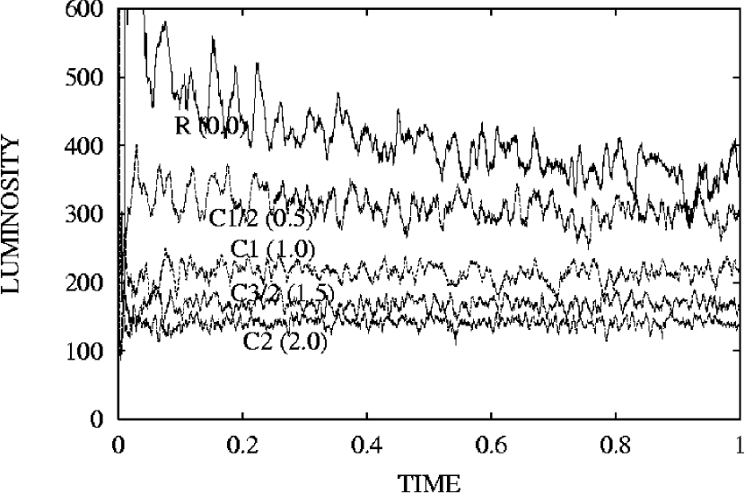
The final configuration reached by the end of 2D dynamical simulations of each of these five models should be the same, since they all correspond to the same physical envelope (the same mass, luminosity and structure below the convection zone). The difference in the simulations is in the relaxation time needed for the different models to adjust their total energy and structure and to reach thermal equilibrium. Due to the long thermal time scale of these envelopes,and to computational limitations, this relaxation phase could not be fully simulated, however, as was demonstrated in figure 1, there was enough data in the beginning of the simulations to reach conclusions about the preferred model.

In this figure the luminosity as a function of time for each of the five simulations was presented. The most obvious result in this figure is that in the simulations that started from models with $\lambda<1$ the envelope lost energy while for simulations started from models with $\lambda>1$ the envelope gained energy. That was the main reason for the conclusion that the 1D model integrated with $\lambda=1$ was the most consistent with the 2D simulations.

A consistency check of this result was done by using 1D dynamic simulation with $\lambda=1$ MLT starting from the above different initial models. It was found out that the 1D simulations mimic the 2D simulations, i.e. the luminosity (and radius) as a function of time for the different initial models looked similar. A more precise analysis of the results revealed that the final configuration of the dynamical simulations (both one and 2D) had slightly less total energy than the static 1D model of $\lambda=1$.

4 More results

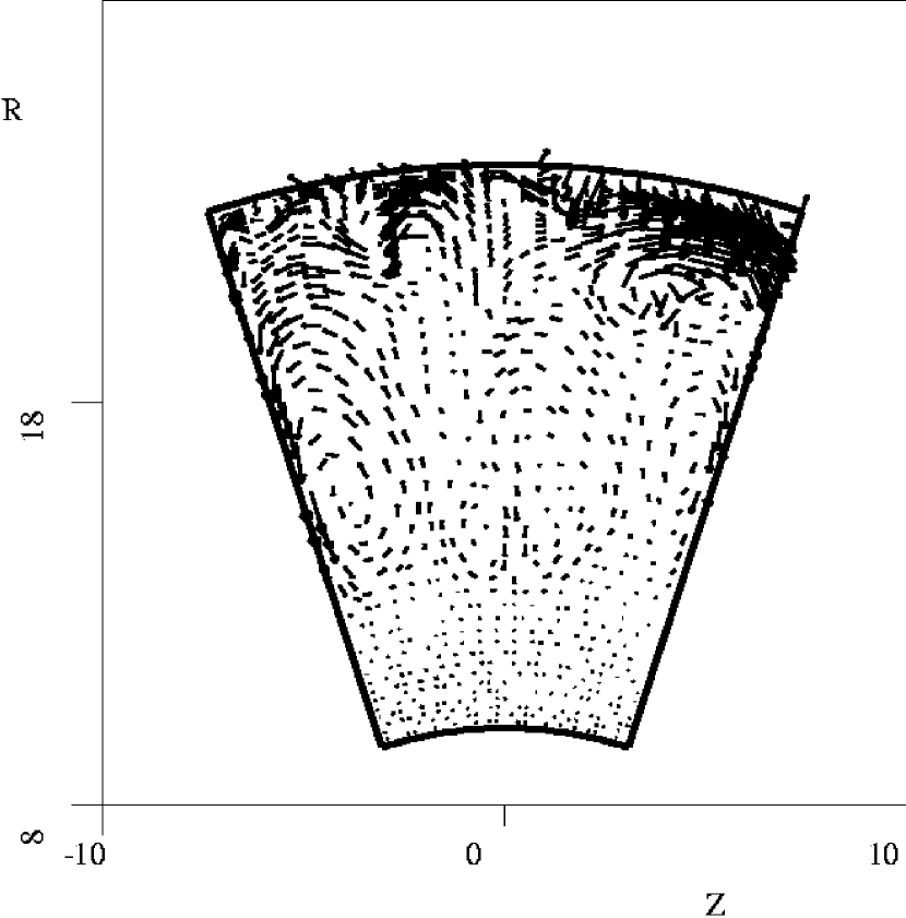
A typical velocity field in the simulations is presented in figure 2. One can identify narrow downstreams and wider upstreams in the flow. The length scale of the streams increased with depth (as well as the pressure scale height). The existence of hydrodynamical waves below the convection zone is apparent.

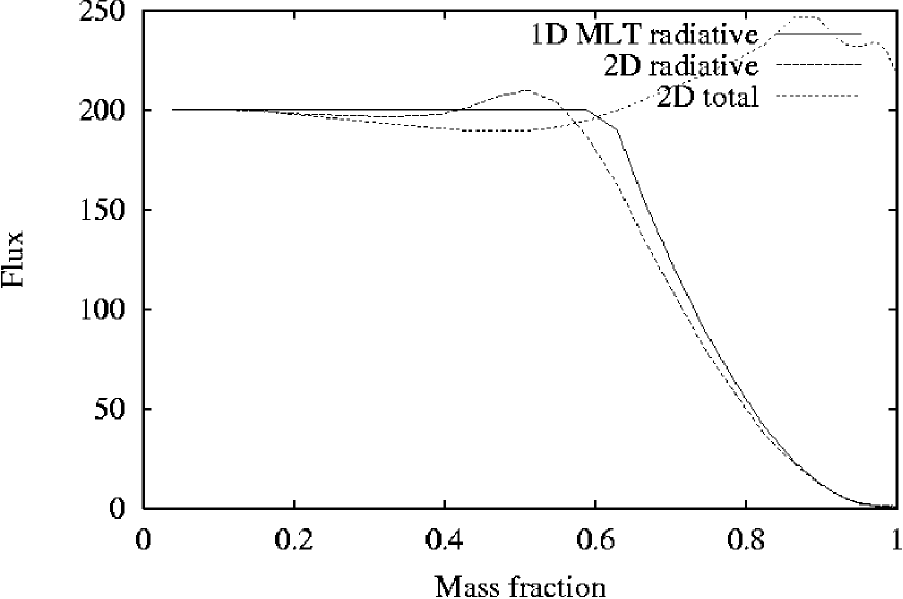
As mentioned before, by comparison of the five simulations a conclusion could be made that the $\lambda=1$ model was the most consistent with the final 2D configuration, however from figure 3 it is clear that this model was not in a full thermal equilibrium. In this figure,the (time) averaged fluxes in the 2D simulation of this model are presented, including the radiative flux and the total flux (the sum of radiative and convective fluxes). For comparison, the 1D (static) radiative flux is presented, too.

The radiative flux in the 2D simulation resembled the static model , though a modest widening of the convective zone is clear, and an increase in the radiative flux above the constant luminosity is apparent near the bottom of the convective zone (see Zahn (1991)). The value of the total flux is indicative of the thermal equilibrium of the model. The total flux was slightly less than $200L_{\sun}$ below the convective zone, and reached a maximum of about $245L_{\sun}$ near the upper boundary and then it declined to the surface luminosity of about $215L_{\sun}$. While it is clear that this is a result of a yet non equilibrium configuration, one shouldn’t forget that due to the lack of algebric energy conservation, this plot is influenced by the uncertainty in the value of the hydrodynamical flux (as was described in §2): The energy conservation in each time step was of the order of $10^{-9}$ of the energy. This seems to be small, but when one divides it by the time step (about 80 seconds), one gets $10L_{\sun}$. I think it is important to note that this has little effect upon the simulation itself, which I confirmed by adding artificial non-energy-conserving term to the 1D dynamic code and comparing the results of several simulations where I changed the value of this term.

The different values of the luminosity in the simulations (figure 1) were dominated by the values of of the outer radii (compare this figure with figure 3 in AT97). In the initial configurations there was a relatively large difference in the effective temperatures: 3675K for $\lambda=0$, 4600K for $\lambda=1$ and 5110K for $\lambda=2$. However, in the dynamical simulations, very quickly (less than a month) the difference shrank dramatically, and the effective temperature became: 4520K, 4600K, and 4650K (for the same models as above) with time fluctuations of about 100K. In other words, using the dynamical simulations, one gets almost immediately, an effective temperature which is very close to the effective temperature of the $\lambda=1$ model. This gives more confidence in the above conclusion that the $\lambda=1$ is the preferred model. The 1D consistency simulations featured the same phenomenon.

5 results of numerical parameter survey

The five (2D) simulations used similar numerical parameters. The grid consisted of 36 angular cells in each row, with 53 to 72 rows (for the simulations of models with $\lambda>1$, I included deeper regions of the envelope - down to eight $R_{\sun}$ - because of the deeper convection zone). The angular sector was $0.2\pi$ near the equatorial plane. The fluxes in the relaxation stage were calculated using a second order donor scheme, and the energy flux consisted of both internal and kinetic energies. I used reflective boundary conditions on the sides of the computational domain. LES viscosity was used, with Smagorinsky coefficient of 0.5 and without entropy diffusion.

I made many tests of the dynamical simulation of the model that started with the $\lambda=1$ profile. I changed the numerical scheme, the number of cells and the angular width of the computational domain and the parameters of the LES terms.

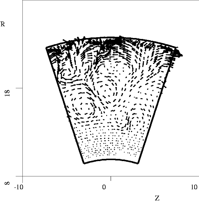
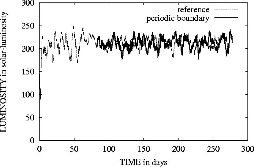
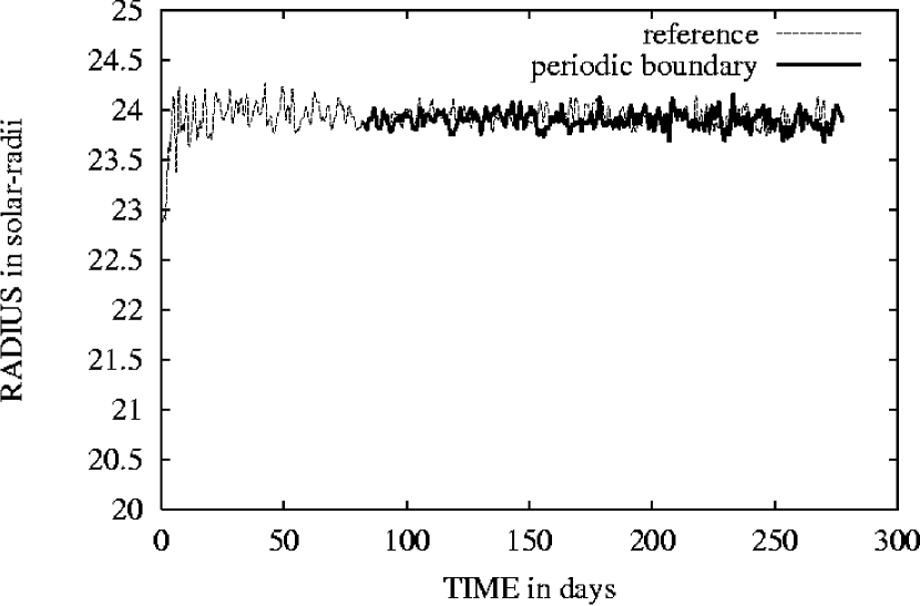
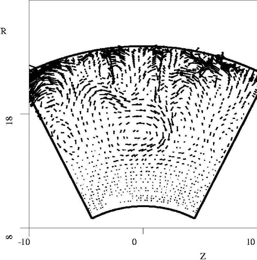
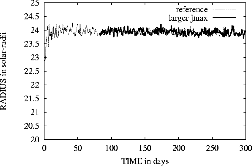
The changes in numerical scheme included: calculating the remapping fluxes using full donor (i.e. without taking the gradients of the hydrodynamical variables into account), using internal energy fluxes in the grid relaxation stage (without adding the kinetic energy) and the use of periodic boundary conditions at the sides. I found that the full donor simulation yielded a rapid expansion of the envelope - implying it is necessary to include gradients in the calculation of the fluxes. The use of the internal energy (only) for the remapping energy fluxes caused a small constant loss of kinetic energy and thus a modest shrinking of the envelope without changing the luminosity. The velocity field of the simulation with periodic boundary conditions is presented in figure 4. The non radial velocities at the sides are expected, but no other significant change can be seen, compared to the velocity field of reflecting boundary conditions (figure 2), i.e. the size of the eddies and the changes in the velocities with depth look similar. The luminosity and outer radius as a function of time look the same as well, as can be seen in figure 5.

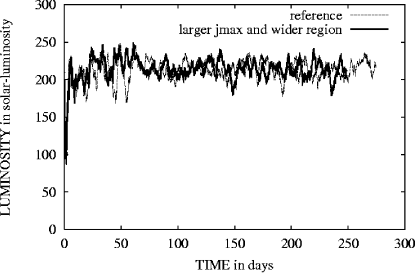
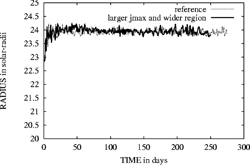
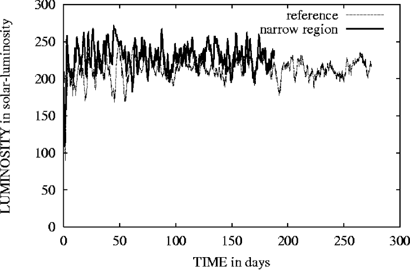
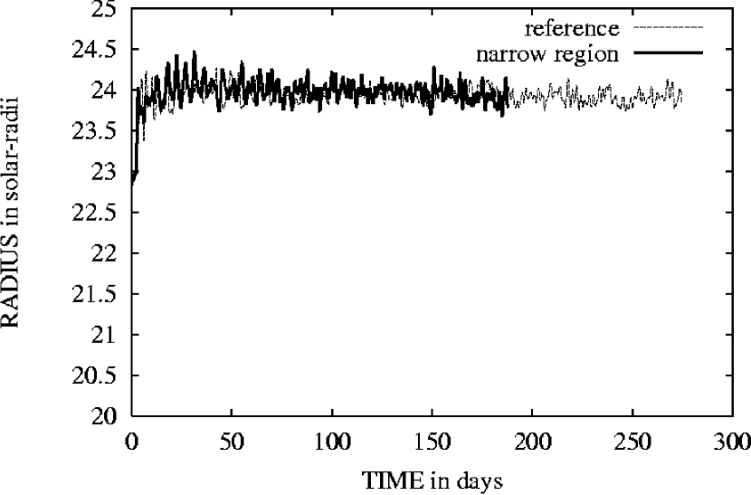
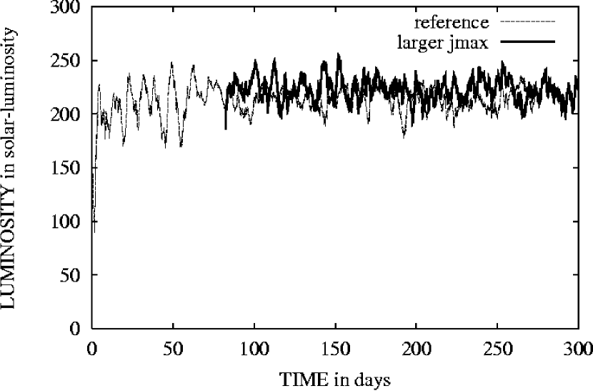
Changes in the angular width or number of cells had small effects. Increasing both the angular width to $0.3\pi$ and the number of cells in each row to 54 yielded similar results as the nominal simulation, as presented in the velocity field - figure 6, and in the luminosity and outer radius - figure 7. When I decreased the angular width to $0.1\pi$ I got a larger variability in the luminosity and outer radius (see figure 8) and a small increase in the average luminosity, as well. A small increase in the average luminosity was seen in a simulation with larger number of cells (=54) in each row (with the nominal angular width of $0.2\pi$), as presented in figure 9. Increasing the number of rows to 81, had no significant effect.

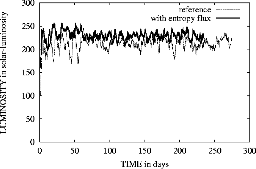
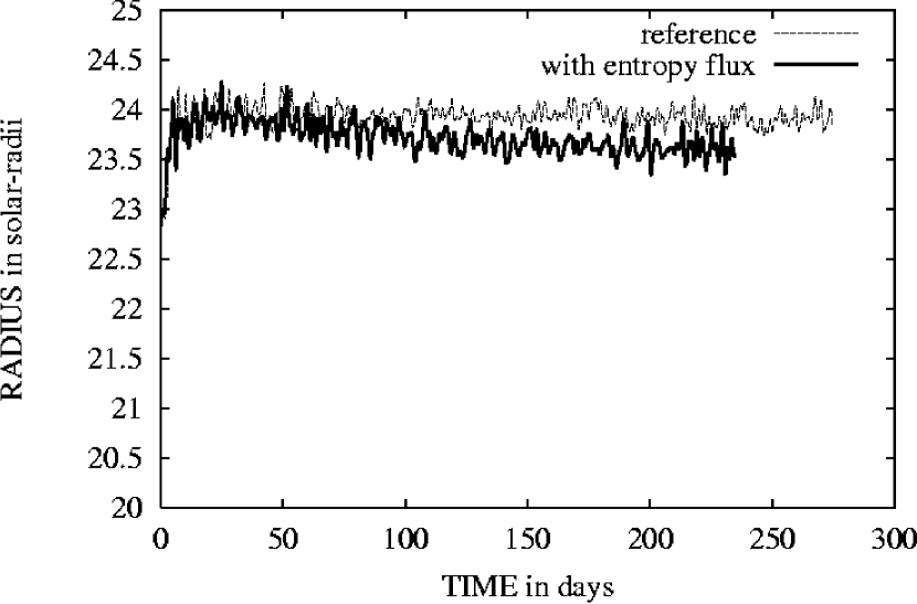
The variations in the LES terms included changing the numerical coefficient and adding an entropy diffusion term. When I had zero or small (Smagorinsky coefficient of 0.01) LES viscosity I got somewhat larger variability in the luminosity and outer radius, but without changes of the average values. However, including an entropy diffusion term (with Prandtl number of one) increased the average luminosity by a small amount (see figure 10). When I had this term, a further increase in the luminosity was evident when the Smagorinsky coefficient was increased to one.

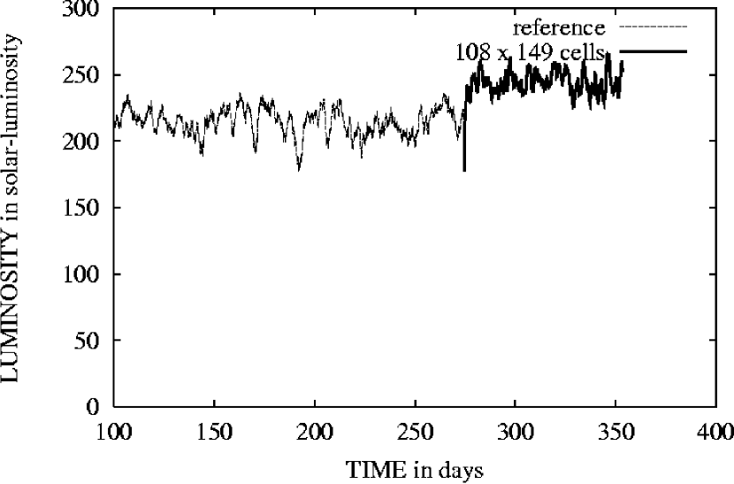
A summary of these tests reveals that there was a tendency to increase the luminosity in two cases: when I increased the angular resolution, and when I added an entropy diffusion term in the LES scheme. These two cases have one physical meaning: an increase in the efficiency of convection by adding smaller scale turbulent fluxes. Since there was a very small luminosity increase in the above simulations, I performed yet another simulation where I increased the resolution by a (relatively) large factor. I started with a profile of the nominal simulation (of $36\times 53$ cells) and increased the number of cells almost by an order of magnitude ($108\times 149$ cells), without the entropy diffusion term. This simulation, being much more CPU demanding, was followed for a small physical time but nevertheless a clear conclusion can be made, as can be seen in figure 11. The luminosity increased quite significantly from about $215L_{\sun}$ in the nominal simulation to about $250L_{\sun}$.

An increase in luminosity means that the envelope loses more energy, and from the five simulation with different initial models, this means that the 1D model which is consistent with the 2D simulations should have a larger value of $\lambda$, i.e. $\lambda>1$. To test this conclusion I performed high resolution simulation starting with the initial model based upon $\lambda=2$. Again, I started with a profile of the nominal simulation (with $36\times 72$ cells) and increased the resolution to $108\times 199$ cells. This yielded an increase in the luminosity from about $140L_{\sun}$ to about $160L_{\sun}$, as expected.

6 Systematic tests for the luminosity

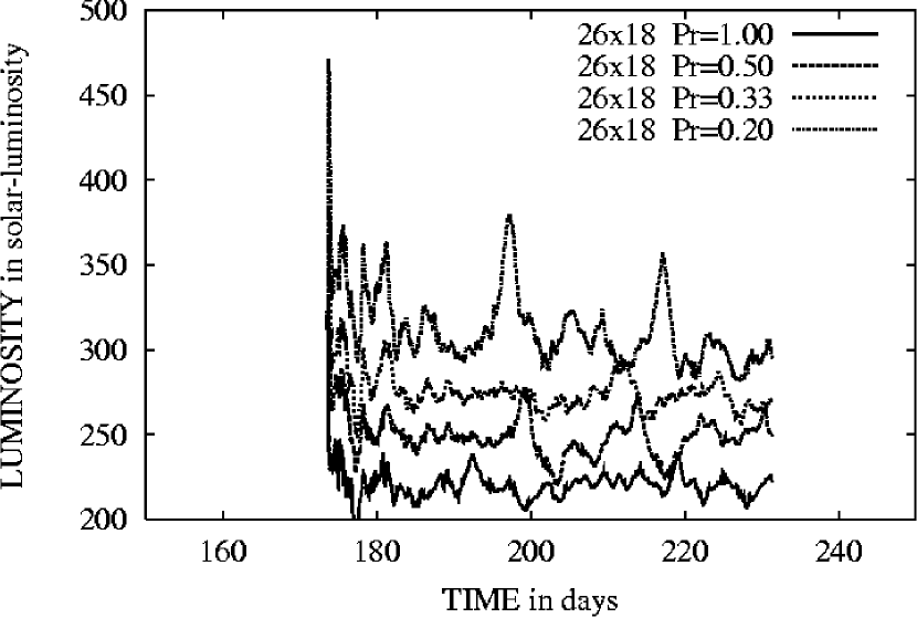
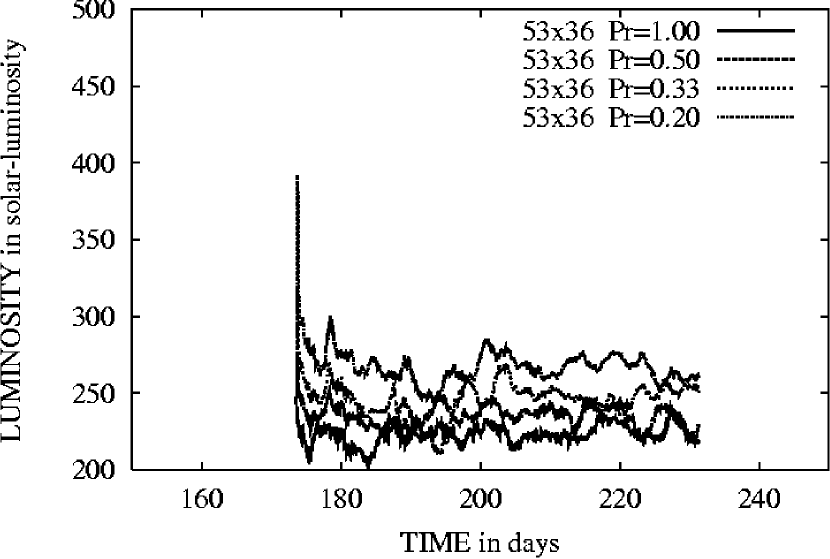
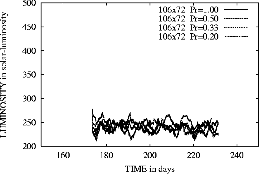
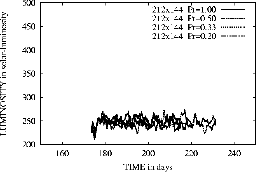
In order to check systematically the dependence of the luminosity in the spatial resolution and in the LES terms, I performed the following simulations, which started with the same initial profile. The initial profile was a 2D profile with an already developed convective flow based on the initial 1D model with $\lambda=1$. From this profile I interpolated four equivalent profiles with different spatial resolution: $18\times 26$ cells, $36\times 53$ cells, $72\times 106$ cells and $144\times 212$ cells, thus having factor of about 64 between the number of cells in the finer grid and in the coarser grid. From the above discussion it is clear that the significant term in the LES scheme is the entropy diffusion term, so I used the nominal 0.5 value of the Smagorinsky coefficient, and changed the importance of the entropy diffusion term by changing the Prandtl number, using the values: $1,\text@frac{1}{2},\text@frac{1}{3},\ {\rm and}\ \text@frac{1}{5}$ (i.e. the last value corresponds to increasing the diffusion term by a factor of five compared to the first value). I used these values of the Prandtl number for each of the four resolutions, and thus having sixteen simulations.

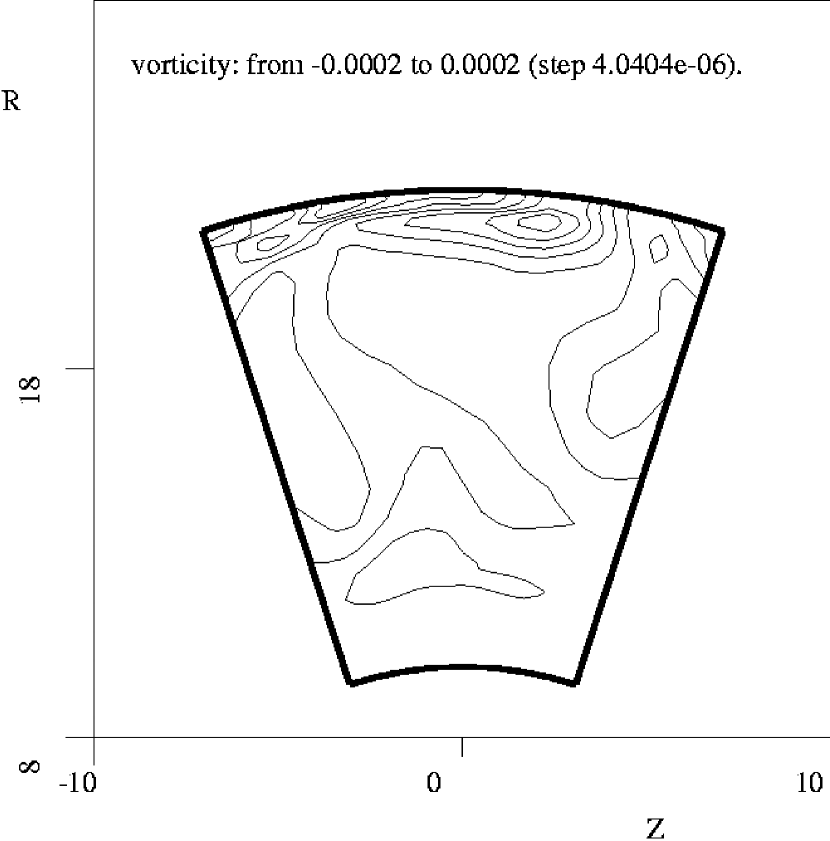
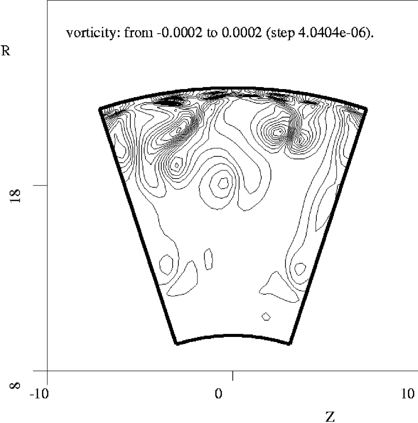
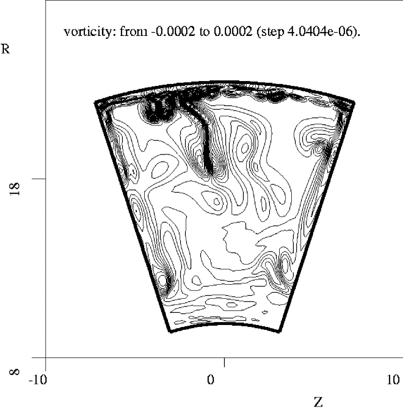
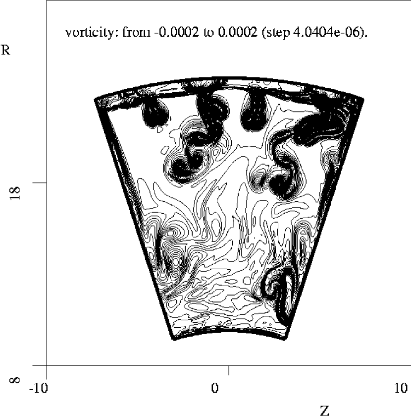
The flow in four of these sixteen simulations is presented in figure 12, for different resolutions. The flow is presented by contours of the vorticity and indeed increasing the resolution yielded more small scale eddies (and higher values of vorticity).

The luminosities of these simulations are summarized in figure 13, and in table 1 I present the average luminosities. From these results one can conclude that the best estimate of the luminosity is $248\pm 2L_{\sun}$, and that the better the resolution is, the less important the value of Prandtl number is. In a perfect LES scheme one should get the converged result for each resolution for given set of numerical parameters (i.e. Prandtl number in our case). However, the value of about $248L_{\sun}$ was obtained in each resolution with a different value of Prandtl number, this value seems to increase when decreasing the resolution.

For two of these 16 simulations I checked the importance of the LES entropy diffusion term comparing to the LES viscosity terms. I performed simulations where I changed both Smagorinsky coefficient and Prandtl number so that the amplitude of the diffusion term would be the same, while changing the amplitude of the viscosity terms. I performed a $72\times 106$ cell simulation with Smagorinsky coefficient of 1.5 and Prandtl number of 1 and got an average luminosity of $242L_{\sun}$ (equivalent to a Prandtl number $\text@frac{1}{3}$ simulation), and a $19\times 26$ cell simulation with Smagorinsky coefficient of 1. and Prandtl number of 1 where I got an average luminosity of $248L_{\sun}$ (equivalent to a Prandtl number $\text@frac{1}{2}$ simulation).

The summary of these results is that the 2D simulations of an initial model calculated with $\lambda=1$ MLT, yields an energy-losing envelope with an average luminosity of $248L_{\sun}$. To find what value of $\lambda$ can reproduce this I performed several 1D dynamic simulations. In each of these simulations, I started with the same $\lambda=1$ profile, and assuming different values for the $\lambda$ in the dynamical model I got different luminosities. For the following values of $\lambda$: 1.2, 1.3, 1.4 and 1.5 I got average luminosities of about: 230, 240, 250 and 270 ($L_{\sun}$). From this I conclude that the consistent value of $\lambda$ is 1.4 .

7 Summary

As was presented in AT97 the convective envelope of a red giant (of mass $1.2M_{\sun}$, core mass of $0.96M_{\sun}$, luminosity of $200L_{\sun}$, and metallicity $Z=0.001$) was studied by comparing 2D simulations of five different initial models. While a full convergence of these simulations to a balanced final configuration was not possible, due to the large thermal time scale of this envelope, it was found that an initial model calculated with MLT using $\lambda=1$, was almost energetically balanced, and thus was the best estimate of the final configuration.

The fast change in the effective temperature obtained in these dynamic simulations, towards the effective temperature of the $\lambda=1$ model is a further indication that this conclusion is consistent.

After a comprehensive survey of the importance of the various parameters used in the simulation technique, a sensitivity to the spatial resolution and to the LES entropy diffusion term was found. This sensitivity was tested by using four resolutions and four values of the LES term, and it was concluded that the preferred value of $\lambda$ is 1.4, for the envelope tested in this study. It was found that ,at least for this code and for these kind of simulations, one needs to calibrate the LES terms.

The conclusion for the value of $\lambda$, to be used in modeling the ged giant envelope studied in this research, being larger than one is consistent with the results of Stothers & Chin (1997) where they calculated evolutionary sequences and compared them to observation. This value of 1.4 is also consistent with extrapolation of the results of Ludwig et al. (1999) and Freytag et al. (1999) where numerical simulations were applied to the outer convective zone of solar like stars.

This conclusion is important for studies in which an accurate modeling of Red Giants is necessary, like obtaining pulsation times of Miras (Yaari & Tuchman (1998)) or calculating isochrones of globular clusters(Freytag & Salaris (1999)).

An obvious limitation of this study is the use of 2D simulations (and not 3D simulations). The spectrum of eddy sizes is probably different in 3D, but the influence of this upon the calibrated mixing length parameter is not known. However, Ludwig et al. (1999) have first estimation of the change in the calibrated mixing length parameter for their study of solar type convection, due to the difference between 2D and 3D simulations. They conclude that the calibrated mixing length parameter for the sun from 3D simulation is higher by 0.07 than from 2D simulation.

Table 1: Average Luminosities ($L_{\sun}$)

$\frac{no.\ of\ cells}{Prandtl\ no.}$	$18\times 26$	$36\times 53$	$72\times 106$	$144\times 212$
$1$	224	225	235	250
$\text@frac{1}{2}$	250	234	239	246
$\text@frac{1}{3}$	272	247	242	248
$\text@frac{1}{5}$	316	265	248	250

Figure 1: Luminosities as a function of time in the 2D simulations of different initial models. The $\lambda$ used to integrate each initial model is indicated. Luminosities are in $L_{\sun}$ and the time is in years.

Figure 2: The velocity field in the $\lambda=1$ standard simulation. Z is the rotation axis and R is the distance from it in $R_{\sun}$, the largest arrows correspond to velocity of $10^{6}\text@frac{cm}{s}$

Figure 3: Energy fluxes in the $\lambda=1$ standard simulation in $L_{\sun}$ as a function of the mass fraction in the simulated envelope. The outer boundary corresponds to mass of $1.2M_{\sun}$, and the total mass of the simulated region is $.013M_{\sun}$. The different flux components are indicated.

Figure 4: The velocity field in the periodic boundary simulation. Z is the rotation axis and R is the distance from it in $R_{\sun}$, the largest arrows correspond to velocity of $10^{6}\text@frac{cm}{s}$

Figure 5: (a) Luminosities ($L_{\sun}$) and (b) outer radii ($R_{\sun}$) as a function of time (days) in the 2D simulation with periodic boundary (bold) and in the standard simulation (dash).

Figure 6: The velocity field in the wider sector simulation. Z is the rotation axis and R is the distance from it in $R_{\sun}$, the largest arrows correspond to velocity of $10^{6}\text@frac{cm}{s}$

Figure 7: (a) Luminosities ($L_{\sun}$) and (b) outer radii ($R_{\sun}$) as a function of time (days) in the 2D simulation with a wider sector (bold) and in the standard simulation (dash).

Figure 8: (a) Luminosities ($L_{\sun}$) and (b) outer radii ($R_{\sun}$) as a function of time (days) in the 2D simulation with a narrow sector (bold) and in the standard simulation (dash).

Figure 9: (a) Luminosities ($L_{\sun}$) and (b) outer radii ($R_{\sun}$) as a function of time (days) in the 2D simulation with more cells in each row (bold) and in the standard simulation (dash).

Figure 10: (a) Luminosities ($L_{\sun}$) and (b) outer radii ($R_{\sun}$) as a function of time (days) in the 2D simulation with LES entropy diffusion term (bold) and in the standard simulation (dash).

Figure 11: Luminosities ($L_{\sun}$) as a function of time (days) in the 2D simulation with $108\times 149$ cells (bold) and in the standard simulation (dash).

Figure 12: Vorticity contours in the (a) $18\times 26$ (b) $36\times 53$ simulations. Z is the rotation axis and R is the distance from it in $R_{\sun}$.

Figure 12 -cont: Vorticity contours in the (c) $72\times 106$ and (d) $144\times 212$ simulations. Z is the rotation axis and R is the distance from it in $R_{\sun}$.

Figure 14: Luminosities ($L_{\sun}$) as a function of time (days) in the 2D simulations with (a) $18\times 26$ (b) $36\times 53$. In each figure the four different Prandtl no. simulations are presented.

Figure 13 -cont: Luminosities ($L_{\sun}$) as a function of time (days) in the 2D simulations with (c) $72\times 106$ and (d) $144\times 212$ cells. In each figure the four different Prandtl no. simulations are presented.

References

- Abbett et al. (1997) Abbett, W.P., Beaner, M., Davids, B., Georgobiani, D., Rathbun, P., & Stein R.F. 1997, ApJ, 480, 395
- Arnett (1994) Arnett, W.D. 1994, ApJ, 427, 932
- Asida & Tuchman (1997) Asida, S.M., & Tuchman, Y. 1997, ApJ, 491, l47
- Basu & Antia (1994) Basu, S. & Antia, H. M. 1994, Journal of Astrophysics and Astronomy, 15, 143
- Bazan & Arnett (1994) Bazan, G., & Arnett, W.D. 1994, ApJ, 433, L41
- Bazan & Arnett (1998) Bazan, G., & Arnett, W.D. 1998, ApJ, 496, 316
- Bogdan et al. (1993) Bogdan, T.J., Cattaneo, F., & Malagoni, A., 1993, ApJ, 407, 316
- Bohm-Vitense (1958) Bohm-Vitense E., 1958, Z. Astrophys. 46, 108
- Buchler et al. (1999) Buchler, J.R., Yecko, P., Kollth, Z., & Goupil, M.-J. 1999, astro-ph/9905025
- Canuto (1996) Canuto, V.M., 1996, ApJ, 467, 385
- Canuto (1997) Canuto, V.M., 1997, ApJ, 482, 827
- Canuto & Christensen (1998) Canuto, V.M., & Christensen-Dalsgaard, J., 1998, Annu. Rev. Fluid Mech., 30, 167
- Canuto & Dubovikov (1998) Canuto, V.M., & Dubovikov, M., 1998, ApJ, 493, 834
- Canuto et al. (1996) Canuto, V.M., Goldman, I., & Mazzitelli, I., 1996, ApJ, 473, 550
- Canuto & Mazzitelli (1991) Canuto, V.M., & Mazzitelli, I., 1991, ApJ, 370, 295
- Castaing et al. (1989) Castaing, B., Gunaratne, G., & Heslot, F., 1989, J. Fluid Mech., 204, 1
- Cattaneo et al. (1991) Cattaneo, F., Brummell, N.H., Toomre, J., Malagoni, A., & Hurlburt, N.E. 1991, ApJ, 370, 282
- Cattaneo et al. (1990) Cattaneo, F., Hurlburt, N.E., & Toomre, J. 1990, ApJ349, L63
- Chan & Gigas (1992) Chan, K.L., & Gigas, D. 1992, ApJ, 389, L87
- Chan & Sofia (1986) Chan, K.L., & Sofia, S. 1986, ApJ, 307, 222
- Chan et al. (1982) Chan, K.L., Sofia, S., & Wolff, C.L. 1982, ApJ, 263, 935
- Cox & Stewart (1970) Cox, A.N., & Stewart, J.N. 1970, ApJS, 19, 243
- Cox & Giuli (1968) Cox, J.P., & Giuli, R.T. 1968, Principles of Stellar Structure (New York: Gordon & Breach)
- Demarque et al. (1997) Demarque. P., Guenther, D.B., & Kim, Y.-C. 1997, ApJ, 474, 790
- Deupree (1975) Deupree, R.G. 1975, ApJ201, 183
- Deupree (1977) Deupree, R.G. 1977, ApJ211, 509
- Deupree (1985) Deupree, R.G. 1985, ApJ296, 160
- Deupree (1998) Deupree, R.G. 1998, ApJ499, 340
- Freytag et al. (1999) Freytag, B., Ludwig, H.-G., & Steffen, M. 1999, in Proceedings contribution to the Workshop on Stellar Structure: “Theory and Tests of Convective Energy Transport” Granada, Spain, 1998, eds. A. Gimenez, E. Guinan, B. Montesinos
- Freytag & Salaris (1999) Freytag, B. & Salaris, M. 1999, ApJ, 513, L49
- Gehmeyr & Winkler (1992) Gehmeyr, M. & Winkler, K. -H. A. 1992, A&A, 253, 92
- Glasner & Livne (1995) Glasner, S.A., & Livne, E. 1995, ApJ, 445, L149
- Glasner et al. (1997) Glasner, S.A., & Livne, E., & Truran, J.W. 1997, ApJ, 475, 754
- Grossman (1996) Grossman, S. A. 1996, MNRAS, 279, 305
- Grossman & Narayan (1993) Grossman, S.A., Narayan, R. 1993, ApJS, 89, 361
- Grossman et al. (1993) Grossman, S.A., Narayan, R., & Arnett, D. 1993, ApJ, 407, 284
- Helsot et al. (1987) Helsot, F., Castaing, B., & Libchaber, A. 1987, Phys. Rev. A, 36, 5870
- Hossain & Mullan (1991) Hossain, M., & Mullan, D.J. 1991, ApJ, 380, 631
- Hurlburt et al. (1984) Hurlburt, N. E., Toomre, J., & Massaguer, J. M. 1984, ApJ, 282, 557
- Hurlburt et al. (1986) Hurlburt, N. E., Toomre, J., & Massaguer, J. M. 1986, ApJ, 311, 563
- Hurlburt et al. (1994) Hurlburt, N. E., Toomre, J. , Massaguer, J. M., & Zahn, J. -P. 1994, ApJ, 421, 245
- Kercek et al. (1998) Kercek, A., Hillebrant, W., & Truran, J.W. 1998, A&A, 337, 379
- Kercek et al. (1999) Kercek, A., Hillebrant, W., & Truran, J.W. 1998, A&A, 345, 831
- Kerr (1996) Kerr, R.M. 1996, J. Fluid Mech., 310, 139
- Kim et al. (1995) Kim, Y. -C. , Fox, P. A., Sofia, S., & Demarque, P. 1995, ApJ, 442, 422
- Kim et al. (1996) Kim, Y. -C. , Fox, P. A., Demarque, P., & Sofia, S. 1996, ApJ, 461, 499
- Livne (1993) Livne, E. 1993, ApJ, 412, 634
- Ludwig et al. (1999) Ludwig, H.-G., Freytag, B., & Steffen, M. 1999 A&A, A&A, 346, 111
- Ludwig et al. (1994) Ludwig, H. -G., Jordan, S. & Steffen, M. 1994, A&A, 284, 105
- Maeder & Conti (1994) Maeder, A., & Conti, P.S. 1994, ARA&A, 32, 227
- Malagoni et al. (1990) Malagoni, A., Cattaneo, F., & Brummell, N.H. 1990, ApJ, 361, L33
- Mezzacappa et al. (1998) Mezzacappa, A., Calder, A. C., Bruenn, S. W., Blondin, J. M., Guidry, M. W., Strayer, M. R. & Umar, A. S. 1998, ApJ, 495, 911
- Mller & Janka (1997) Mller, E., & Janka H.-T. 1997, A&A, 317, 140
- Nordlund & Stein (1995) Nordlund, A., & Stein, R.F. 1995, Stellar Evolution: What can be Done, 32nd Liege Int. Astroph. Coll.
- Nordlund et al. (1996) Nordlund, A., Stein, R.F., & Brandenburg, A. 1996, Bull Astron. Soc. India, 24
- Paczinski (1969) Paczinski, B. 1969, Acta Astr. 19, 1
- Porter & Woodward (1994) Porter, D.H., & Woodward, P.R. 1994, ApJS, 93, 309
- Rast and Toomre (1993) Rast, M.P.,& Toomre, J. 1993, ApJ, 419, 224
- Schwarzchild (1961) Schwarzchild, M. 1961, ApJ, 134, 1
- Singh & Chan (1993) Singh, H. P., & Chan, K. L. 1993, A&A, 279, 107
- Singh et.al (1994) Singh, H. P., Roxburgh, I. W., & Chan, K. L. 1994, A&A, 281, L73
- Singh et.al (1995) Singh, H. P., Roxburgh, I. W., & Chan, K. L. 1995, A&A, 295, 703
- Smagorinsky (1963) Smagorinsky, j. 1963, Mon. Weather Rev., 91(3), 99
- Smalley & Kupka (1997) Smalley, B., & Kupka, F. 1997, A&A, 328, 349
- Spiegel (1963) Spiegel, E.A. 1963, ApJ, 138, 216
- Spruit et al. (1990) Spruit, H.C., Nordlund, A., & Title, A.M. 1990, ARA&A, 28, 263
- Stein & Nordlund (1989) Stein R.F., & Nordlund, A. 1989 ApJ, 342, L95
- Stein & Nordlund (1998) Stein R.F., & Nordlund, A. 1998 ApJ, 499, 914
- Stellingwerf (1982) Stellingwerf, R.F. 1982, ApJ, 262, 330
- Stone and Balbus (1996) Stone, J. M., & Balbus, S. A. 1996, ApJ, 464, 364
- Stothers & Chin (1995) Stothers, R. B., & Chin, C. -W. 1995, ApJ, 440, 297
- Stothers & Chin (1997) Stothers, R. B., & Chin, C. -W. 1997, ApJ, 478, L103
- Tligner et al. (1993) Tligner, A., Belmonte, A., & Libchaber, A. 1993, Phys. Rev. E, 47, R2253
- Tuchman (1980) Tuchman, Y. 1980, “Dynamical Phenomena in Red Giant Envelopes”, Phd. thesis
- Tuchman et al. (1978) Tuchman, Y., Sack, N., & Barkat, Z. 1978, ApJ, 219, 183
- Tuchman et al. (1979) Tuchman, Y., Sack, N., & Barkat, Z. 1979, ApJ, 234, 217
- Ulrich (1970) Ulrich, R.K. 1970, Ap. Space Sci., 7, 71
- Ulrich (1976) Ulrich, R.K. 1976, ApJ, 207, 564
- van Leer (1979) van Leer B. 1979, J. Comput. Phys., 32, 101
- Werne (1993) Werne, J. 1993, Phys. Rev. E, 48, 1020
- Werne (1994) Werne, J. 1994, Phys. Rev. E, 49, 4072
- Wu & Libchaber (1992) Wu, X.-Z., & Libchaber, A. 1992, Phys. Rev. E, 45, 842
- Xie & Toomre (1993) Xie, X., & Toomre, J. 1993, ApJ, 405, 747
- Xiong et al. (1997) Xiong, D. R., Cheng, Q. L., & Deng, L. 1997, ApJS, 108, 529
- Xiong et al. (1998a) Xiong, D. R., Deng, L., & Cheng, Q. L. 1998, ApJ, 499, 355
- Xiong et al. (1998b) Xiong, D. R., Cheng, Q. L., & Deng, L. 1998, ApJ, 500, 449
- Yaari & Tuchman (1998) Yaari, A., & Tuchman, Y. 1998, private communication
- Zahn (1991) Zahn, J. -P. 1991, A&A, 252, 179