Two-Dimensional Line Strength Maps in Three Well-studied Early-Type Galaxies

Abstract

Integral field spectroscopy has been obtained for the nuclear regions of 3 large, well-studied, early-type galaxies. From these spectra we have obtained line strength maps for about 20 absorption lines, mostly belonging to the Lick system. An extensive comparison with multi-lenslet spectroscopy shows that accurate kinematic maps can be obtained, and also reproducible line strength maps. Comparison with long-slit spectroscopy also produces good agreement.

We show that Mg is enhanced with respect to Fe in the inner disk of one of the three galaxies studied, the Sombrero. [Mg/Fe] there is larger than in the rest of the bulge. The large values of Mg/Fe in the central disk are consistent with the centres of other early-type galaxies, and not with large disks, like the disk of our Galaxy, where [Mg/Fe] $\sim$ 0. We confirm with this observation a recent result of Worthey (1998) that Mg/Fe is determined by the central kinetic energy, or escape velocity, of the stars, only, and not by the formation time scale of the stars.

A stellar population analysis using the models of Vazdekis et al. (1996) shows that our observed H$\gamma$ agrees well with what is predicted based on the other lines. Given the fact that H$\beta$ is often contaminated by emission lines we confirm the statement of Worthey & Ottaviani (1997), Kuntschner & Davies (1998) and others that if one tries to measure ages of galaxies H$\gamma$ is a much better index to use than H$\beta$. Using the line strength of the Ca II IR triplet as an indicator of the abundance of Ca, we find that Ca follows Fe, and not Mg, in these galaxies. This is peculiar, given the fact that Ca is an $\alpha$-element. Finally, by combining the results of this paper with those of Vazdekis et al. (1997) we find that the line strength gradients in the three galaxies are primarily caused by variations in metallicity.

1 Introduction

The study of the stellar populations of local galaxies plays a major role in understanding galaxy formation and evolution, not in the least because we can only understand high-redshift galaxies by comparing them to the local universe. In recent years significant progress has been made in understanding the stellar populations of nearby galaxies, for ellipticals as well as spirals. Elliptical galaxies are found to fit well single-age, single-metallicity (SSP) models (e.g. Bruzual & Charlot 1993, Worthey 1994, Vazdekis et al. 1996), suggesting that most stars that we currently see were formed on a small time scale. Large ellipticals generally have non-solar Mg/Fe ratios (Peletier 1989, Worthey et al. 1992), while it appears that there is a large spread in age among them (González 1993), although this is not generally accepted (see Kuntschner & Davies 1998). Spiral galaxies have been less well studied, because of the presence of extinction and star formation makes stellar population studies much more difficult. Recent reviews about the stellar populations in bulges, and their differences with ellipticals, are, e.g., Worthey (1998) and Peletier (1999).

This paper is part of a series of papers, with the aim of studying galactic bulges in the same detail as ellipticals. To do this, we have first developed a new spectrophotometric stellar population model, that can be used to interpret observed colours and absorption lines of galaxies (Vazdekis et al. 1996, hereinafter Paper I). To test this model, we have presented in a subsequent paper high-quality long-slit observations of three representative early-type galaxies, in many lines and colours, and applied the model to it. This allowed us to obtain a detailed understanding of ages and abundance distributions of these well-studied, ’standard’, galaxies (Vazdekis et al. 1997, hereinafter Paper II). In the current paper, we again present the same three galaxies (NGC 3379, NGC 4472 and NGC 4594) but now using two-dimensional data, derived using Integral Field Spectroscopy (IFS). This is the first time a detailed study has been performed of galaxy absorption line strengths using a multi-fiber instrument. A similar, but much more limited study has been performed by Emsellem et al. (1996), who used the multi-lenses IFU system TIGER on the CFHT to obtain 2-dimensional kinematic and line strength maps of the Sombrero galaxy. Although the number of absorption lines studied by them is much smaller, their paper offers us an excellent opportunity to carefully check our IFU results. Two-dimensional spectroscopy of early-type galaxies has also been obtained by Sil’chenko and collaborators (e.g. Sil’chenko et al. 1997, 1999), but in their papers only two-dimensional kinematics has been presented.

There are several advantages in using IFS as opposed to multiple long slit spectra. Once the problems of data reduction have been overcome, the larger spatial coverage will be a great advantage in studying is much the galaxy kinematics. For example, one can study the triaxiality of a system much better than using long slits (see e.g. Statler 1991). Studying e.g. whether photometric and kinematic centres coincide is now much easier. With regard to stellar populations: one can find two-dimensional stellar population structures, like young disks and remnants of mergers, purely by analyzing line strength maps. One can detect small amounts of star formation everywhere in the area covered. And, compared to long-slit spectroscopy, the sensitivity at a certain radius is much larger, since more area is covered. We will discuss in this paper results obtained using a fiber bundle of 125 fibers. In the near future however, thousands of fibers will be used, which undoubtedly will make IFS much more popular and important than it is at present.

In this paper, several tests will be presented to establish our IFS reduction techniques. But also, we will present some entirely new data, for the H$\gamma$ line, and for the Ca II IR triplet. H$\gamma$ is a good age-indicator, when used together with e.g. Mg₂ (Worthey & Ottaviani 1997), and can be used even when H$\beta$ is filled in by emission. The Ca II IR triplet in the near-infrared is one of the few lines depending strongly on stellar surface gravity (see e.g. Carter et al. 1987), allowing us to possibly measure or constrain the IMF slope. In this paper we present the Ca triplet (which we will address as Ca T in the rest of this paper) calibrated using stars of Díaz et al. (1989).

We will present very little kinematics here, only a comparison with Emsellem et al. (1996), to show the reliability of our velocity dispersion corrections. Kinematics, including line profile analysis, will be presented in a future paper (Prada et al. 1999, in preparation). Here we present stellar population analysis of the 3 well-studied galaxies. At the same time, we also observed 2 other galaxies: the dwarf elliptical M 32 and the Sb NGC 2841. The analysis of these two galaxies will also be presented in future papers. The organization of our paper is as follows. In Section 2 the observations are described. In Section 3 we described the data reduction. In Section 4 a comparison is made with Paper II and Emsellem et al. (1996). In Section 5 we present our results, amongst other the population synthesis. In the last Section our conclusions are given.

2 Observations

2.1 The Instrument

The data analyzed in this paper were obtained on Feb. 15-17, 1997, at the Observatorio del Roque de los Muchachos, on the island of La Palma. We used the 2D-FIS (Two-dimensional Fiber ISIS System), which is placed between the f/11 Cassegrain focus of the 4.2 m William Herschel Telescope (WHT) and the ISIS double spectrograph. A detailed technical description is provided by García et al. (1994); here we will only recall its main characteristics. The core of the system consists of a 2.5 m long bundle formed by 125 optical fibers, each 200 $\mu$m (0.9” on the sky) in diameter, arranged in two groups in the focal plane. One has 95 fibers, forming an array 9.4” $\times$ 12.2” on the sky, while the other, a ring of 38” in radius with 30 fibers, is intended to collect the background light. The relative positions of the fibers at the telescope’s focal plane are known very accurately, the distance between two adjacent fibers being about 1.1”. Figure 1 shows the actual distribution of the fibers in the central rectangle. At the slit the fibers have been arranged linearly (with a distance of 425 $\mu$m between adjacent fibers). With this type of arrangement, a set of spectra - corresponding to 125 zones in the circumnuclear region - is recorded in each exposure. The advantage of the system as opposed to, say, a Fabry-Perot is that all the spectral and spatial information is recorded simultaneously and that the spectral coverage is determined by the spectrograph alone. Details on the technique itself may be found in Arribas, Mediavilla, & Rasilla (1991), and references therein.

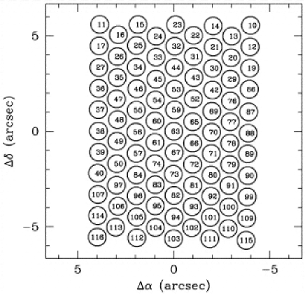
Figure 1: Spatial distribution of the fiber faces of the central rectangle of the optical fiber bundle, at the 4.2 m WHT focal plane. The central fiber (labeled 63) is the origin of the coordinate axes. North is at the top and east is to the left. The numbers reflect the order of the fibers on the entrance slit.

2.2 Our Observations

The observations were made using simultaneously the blue and red arms of the ISIS double spectrograph. In the blue arm, the R300 grating was used, giving us a pixel scale of 96 km/s (1.55 ${\rm\AA}$), a range between 4100 and 5650 ${\rm\AA}$, covering most of the lines of the Lick system, including H$\gamma$ (Worthey & Ottaviani 1997), and a resolution of 2 pixels. In the red, we centered our spectrum on the Ca T. Here we had a pixel size of 28 km/s (resolution 2 pixels) and a spectral range from 8200 to 9000 ${\rm\AA}$. On both arms 1024 $\times$ 1024 thinned TEK CCDs were used. A dicroic, centered at 6100 ${\rm\AA}$, was used, and in the red arm a GG495 order sorting filter was placed as well. Weather conditions during the first two nights, during which the three galaxies were observed, were photometric, with a seeing of $\approx$ 1”. A log of the observations is presented in Table 1.

Table 1: Observation Log

Galaxy	Date	total tint
NGC 4594 (Sombrero)	15 Feb	9000s
NGC 3379	16 Feb	10800s
NGC 4472	16 Feb	7200s

Each night, we also observed some out-of-focus standard stars, using the same setup. In total 20 stars were observed.

3 Data Reduction

Since observations of this type are not very common, and some steps of the data reduction process are significantly different from reducing e.g. long-slit data, we will cover the reduction process in quite some detail, and describe a number of tests showing that our results are reliable. To summarize, we first extract the light in the individual galaxy fibers after removing the stray light between the fibers. We then correct each fiber for its relative transmission using a twilight sky image, and correct for pixel to pixel sensitivity variations using tungsten lamp flatfields. After this we calibrate the spectra in wavelength using CuAr arc lamp exposures, remove cosmic rays, and subtract the sky background. We then extract for each fiber absorption line indices as well as kinematic information, and make maps of these. All of this work was done in IRAF, with some programs written by ourselves. Here we describe these steps in more detail.

3.1 Stray Light

The first reduction step was to remove the stray light. This light has a diluting effect on the spectra, making it more difficult to measure line indices of the object. For 2D-FIS the individual fibers are well separated along the spatial direction of the CCD detector: the distance between adjacent fibers is 6 pixels, and the aperture width is 4 pixels. In Fig. 2 a cut along the spatial direction shows the relative separations of the fibers. For this set up, the optical cross-talk (contamination on a fiber due to the wings of the nearer fibers) is negligible if the difference in intensity between adjacent fibers is not too large. This is the case for most objects, except in focus standard stars. The object images are not very much affected by cross-talk because the fibers are conveniently ordered along the spectrograph slit. We determined the stray light to be subtracted by fitting legendre polynomia through the spatial regions between the fibers, and subtracted it. Subtracting stray light however barely affects the final line indices. This is mostly due to the fact that the galaxy light across the frame doesn’t vary very much, so that an addition of a few percent of light from elsewhere in the galaxy will not affect the integrated line index. Experimentally we found that for the Sombrero in the blue the average values of the line indices did not change by more than 0.2 ${\rm\AA}$. The RMS fiber difference between correcting and not correcting for stray light was about 0.3 ${\rm\AA}$ per index (0.005 for Mg₁ and Mg₂), of the same order as the numbers in Table 3, indicating that by correcting for stray light we might improve the data. For that reason the correction has been applied, although it remains uncertain whether it was really necessary.

Figure 2: First $\sim$ 30 fibers along the slit in the blue of the Sombrero galaxy, showing the positions of the individual fibers. The first 9 fibers belong to the outer ring to measure the sky background.

3.2 Flatfielding and Extracting the Fibers

Flatfielding was done to remove sensitivity variations from pixel to pixel of the system, and fiber to fiber transmission variations. The TEK CCDs that we used suffer considerably from fringing in the red (Peletier 1996), but also in the blue, all the way up to 5000 ${\rm\AA}$. We measure fringing amplitudes of about 10% in our whole red region and between 4200 and 4400 ${\rm\AA}$, and about 5% between 4400 and 5000 ${\rm\AA}$. As explained in the technical note, this fringing depends only on the position of the telescope, and can be corrected for very well. For measuring maps of very tiny absorption lines however, our final accuracy might be determined by how well we can correct for this fringing. At the position of each object, star and galaxy, we also measured a Tungsten flatfield, and used this to correct for the fringing. The flatfield image was corrected for stray light, after which the fibers spectra were extracted. To the extracted spectra polynomials (10th order in the blue and 3rd order in the red) were fitted, in order to correct for the spectral response of the Tungsten lamp, but not for the fringes. Following this the object fibers (galaxy or star) were extracted using the flatfield image as a tracer. This is justified because flat and object (and arc) images are observed at the same position of telescope and then the shifts of each fiber are negligible. They were then divided by the normalized flatfield, and following that each fiber was divided by its relative transmission, determined from twilight sky frames taken at the beginning and end of each night.

3.3 Wavelength Calibration, Cosmic Ray and Background Removal

Wavelength calibration was done using CuAr arc lamp exposures taken before or after each object frame. For each fiber separately the corresponding arc spectrum was extracted, and low order polynomials were fitted to pixel positions of the arc lines as a function of wavelength. On the average the accuracy of the fit for an arc line was 0.08 ${\rm\AA}$ (4.8 km/s) in the blue and 0.05 ${\rm\AA}$ (1.7 km/s) in the red. Using these polynomials the spectra were rebinned in log(lambda). Since for all of our galaxy we had observed at least 4 data frames of 1800s each, we could combine them and remove the cosmic rays with a simple median filtering technique. For the stars, for which only one exposure was taken, very few cosmic rays were present because of their short exposure times, and these were removed using a sigma-clipping algorithm. We then proceeded to subtract the sky background. Two methods were tested. We took separate sky exposures before and after the galaxy exposures. These were scaled to the galaxy integration time and subtracted. The second method was to take all the fibers in the outer ring together to determine an average sky spectrum, and to subtract that from the galaxy fiber spectra. The first method suffers from the fact that the sky varies with time, so that the sky spectra have to be scaled in some way. Using the second method one has the problem that the outer ring fibers still have some galaxy contribution in them. In our worst case, in NGC 4472, at 38” the galaxy is about 15 $\times$ fainter than at 10” (Peletier et al. 1990), so some contamination of the spectra in the outer regions can be expected. However in these three objects colour and line strength gradients are so small (Peletier et al. 1990, Paper II, González 1993) that such a small contamination of max. 6% will not be noticed. In the blue the sky background in the continuum is so low compared to the galaxies that no trace of it was left after subtracting. In the red the sky subtraction also was very precise, because the continuum flux of the outer parts of the galaxies was always at least 8 times larger than the background. In the region of the Ca II IR triplet there are no sharp emission features in the sky background, only a broad emission line from O2 (Nelson & Whittle 1995).

3.4 Making Maps and Datacubes

On the now reduced spectra we continued to measure absorption line strengths. This was done by first determining the stellar radial velocity and velocity dispersion of each fiber, deredshifting it, measuring equivalent widths as explained e.g. in Paper II and Worthey (1994), calibrating these equivalent widths to put them onto the Lick system in the blue (Faber et al. 1985, Gorgas et al. 1993, Worthey et al. 1994) and the system of Díaz et al. (1989) in the red, and making two-dimensional maps of each of them.

Velocities and velocity dispersions were determined using Bender’s (1990) Fourier Quotient method. A comparison with the literature for the Sombrero galaxy is given in the following section. After deredshifting the spectra using these velocities, indices were determined, which then had to be corrected for velocity broadening. To calibrate this velocity dispersion correction we used our 20 stars (for each star the average of all fibers was taken), and determined for each index a velocity dispersion correction curve (as described in Paper II). The same was done in the blue and in the red. In Table 2 our index definitions are given. We found that the Ca T indices were affected very much by the fact that the two continuum bands were very far from the feature, so that the line strengths of the features are severely affected by small variations in the continuum. For that reason we also tried a few different definitions for the 3 lines of the triplet, from studies of galactic globular clusters. Three other definitions were adopted, from Armandroff & Zinn (1988), Armandroff & da Costa (1991) and Rutledge et al. (1997) (see Table 2).

Table 2: Index definitions

Name	Left Cont.		Band		Right Cont.		Ref.
Blue
Ca 4227	4211.000	4219.750	4222.250	4234.750	4241.000	4251.000	Lick
G 4300	4266.375	4282.625	4281.375	4316.375	4318.875	4335.125	Lick
Fe 4383	4359.125	4370.375	4369.125	4420.375	4442.875	4455.375	Lick
Ca 4455	4445.875	4454.625	4452.125	4474.625	4477.125	4492.125	Lick
Fe 4531	4504.250	4514.250	4514.25	4559.25	4560.50	4579.25	Lick
C2 4668	4611.500	4630.250	4634.00	4720.25	4742.75	4756.50	Lick
H$\beta$	4827.875	4847.875	4847.875	4876.625	4876.625	4891.625	Lick
Fe 5015	4946.500	4977.750	4977.75	5054.00	5054.00	5065.25	Lick
Mg b	5142.625	5161.375	5160.125	5192.625	5191.375	5206.375	Lick
Fe 5270	5233.150	5248.150	5245.65	5285.65	5285.65	5318.15	Lick
Fe 5335	5304.625	5315.875	5312.125	5352.125	5353.375	5363.375	Lick
Fe 5406	5376.250	5387.500	5387.50	5415.00	5415.00	5425.00	Lick
Mg1	4895.125	4957.625	5069.125	5134.125	5301.125	5366.125	Lick
Mg2	4895.125	4957.625	5154.125	5196.625	5301.125	5366.125	Lick
H$\gamma$a	4283.50	4319.75	4319.75	4363.50	4367.25	4419.75	WO97
H$\gamma$f	4283.50	4319.75	4331.25	4352.25	4354.75	4384.75	WO97
Red
Ca 1	8447.5	8462.5	8483	8513	8842.5	8857.5	Diaz et al. 1989
Ca 2	8447.5	8462.5	8527	8557	8842.5	8857.5	Diaz et al. 1989
Ca 3	8447.5	8462.5	8647	8677	8842.5	8857.5	Diaz et al. 1989
CaAZ1	8474.0	8489.0	8490.0	8506.0	8521.0	8531.0	Armandroff & Zinn 1988
CaAZ2	8521.0	8531.0	8532.0	8552.0	8555.0	8595.0	Armandroff & Zinn 1988
CaAZ3	8626.0	8650.0	8653.0	8671.0	8695.0	8725.0	Armandroff & Zinn 1988
CaAD1	8474.0	8489.0	8532.0	8552.0	8559.0	8595.0	Armandroff & Da Costa 1991
CaAD2	8626.0	8647.0	8653.0	8671.0	8695.0	8754.0	Armandroff & Da Costa 1991
CaTP1	8346.0	8489.0	8490.0	8506.0	8563.0	8642.0	Rutledge et al. 1997
CaTP2	8346.0	8489.0	8532.0	8552.0	8563.0	8642.0	Rutledge et al. 1997
CaTP3	8563.0	8642.0	8653.0	8671.0	8697.0	8754.0	Rutledge et al. 1997

Due to the fact that neither the stars on the Lick and Díaz systems are flux calibrated, nor our own spectra, we had to put our observations onto these systems using standard stars. To do this, we took maps of out-of-focus stars,measured their average line indices, and determined for each index a linear relation between the literature index and our measurements. In the red only a single offset was sufficient. In the blue our sensitivity curve is considerably different from that of the Lick IDS, used to define the Lick system, and therefore the conversions are somewhat more complicated. The calibration relations are given in Table 3. The RMS scatter now indicates how accurate our indices are in absolute terms. As one can see from Table 3, the RMS scatter is similar to the scatter for the Lick system itself (see Worthey et al. 1994, Table 1), which implies that the absolute values of our line indices are probably better than those of the Lick system.

Table 3: Conversion to the Lick/Diaz system. Coefficients are given of the equation O = a + b C, with O the observed index and C the calibrated index. There errors in a and b are derived from the dispersion in the stars. $\sigma_{RMS}$ is the RMS dispersion in this relation for a line strength measurement of an individual star. In the last column the RMS dispersion from fiber to fiber in each line index, from observations of defocussed stars, is given.

Band	a	$\pm$	b	$\pm$	$\sigma_{RMS}$	$\sigma_{FF}$
Ca 4227	0.19	0.08	1.40	0.04	0.17	0.260
G 4300	0.55	0.16	1.05	0.03	0.45	0.330
Fe 4383	-0.23	0.42	1.04	0.07	0.83	0.838
Ca 4455	-0.12	0.09	1.21	0.05	0.36	0.191
Fe 4531	0.94	0.23	0.84	0.05	0.48	0.428
C2 4668	0.67	0.32	0.94	0.05	0.76	0.896
H$\beta$	0.125	0.073	1.10	0.02	0.30	0.217
Fe 5015	0.62	0.27	1.02	0.04	0.63	0.495
Mg b	0.007	0.094	1.06	0.03	0.17	0.218
Fe 5270	0.16	0.15	1.00	0.05	0.35	0.280
Fe 5335	0.28	0.15	1.12	0.05	0.34	0.307
Fe 5406	0.29	0.10	1.02	0.05	0.21	0.244
Mg1	-0.044	0.003	0.95	0.02	0.009	0.0090
Mg2	-0.050	0.004	0.98	0.01	0.010	0.0102
H$\gamma$a	-0.32	0.19	0.95	0.02	0.86	0.753
H$\gamma$f	0.000	0.066	1.15	0.02	0.39	0.287
Ca 1	0.157	-	-	-	0.194	0.812
Ca 2	0.454	-	-	-	0.260	0.779
Ca 3	0.512	-	-	-	0.413	0.785
CaAZ1	-	-	-	-	-	0.365
CaAZ2	-	-	-	-	-	0.381
CaAZ3	-	-	-	-	-	0.369
CaAD1	-	-	-	-	-	0.429
CaAD2	-	-	-	-	-	0.386
CaTP1	-	-	-	-	-	0.389
CaTP2	-	-	-	-	-	0.428
CaTP3	-	-	-	-	-	0.387

Having established the accuracy of our average fiber measurement, we then investigated systematic fiber-to-fiber differences using out-of-focus stars. In principle differences in spectral response can occur because each of the fibers sees a different area of the primary mirror, but moving the out-of-focus stars slightly in the focal plane showed that this effect was negligible. The out of focus stars were reduced, and for each fiber absorption line indices were determined. Taking all the fibers for which the integrated flux was larger than 30% of the flux of the brightest fiber we determined the RMS scatter in the line indices for each star, after applying a 3$\sigma$ rejection algorithm. These values are given in the last column in Table 3. The RMS scatter that we found only slightly depends on the signal-to-noise ratio in the stars, showing that these fiber-to-fiber differences are due to some systematic effect. Careful inspection of the data shows that fringing is important in the data, especially in the red, but also somewhat in the blue, and that incorrect flatfielding can affect the values of the indices severely. We therefore think that residual fringing (which is dependent on the position of the telescope) might be responsible for our small residual variations, although it is not excluded that variations in fiber stresses leading to small variations in the continuum could also be responsible. Structures smaller than this level in our maps should probably not be believed. The RMS fiber to fiber differences are on the order of 0.3 ${\rm\AA}$ and 0.010 for the indices expressed in magnitudes. This means that very small gradients are hard to determine, but in general this accuracy is good enough to obtain results of the quality currently produced in the literature (see the comparison with Paper II in the next section).

As a last step we determine maps for each absorption line index, as well as for the integrated continuum, radial velocity, velocity dispersion and higher order velocity moments. The kinematics will be described in a following article (Prada et al. 1999, in preparation). Maps were reconstructed using triangular interpolation and regridded to frames with a pixelsize of 0.48”. Since the data are undersampled the maps will contain some small amount of aliasing. However, the comparison of the reconstructed intensity maps with HST data (see Section 4.1) shows that this is minor and hard to detect. We see however that in the three galaxies the position of the galaxy center in the red is somewhat different from in the blue. This is due to differential refraction (see for an example Arribas et al. 1997). The differential refraction within the red or blue band however was so small compared to the spatial resolution that we didn’t correct for it. To give an idea about the final obtained resolution Arribas et al. (1997) looked at reconstructed images of in focus stars, and found them to have FWHM values of 1.2”. For the data in this paper the analysis of Section 4.1 shows that similar values have been obtained here.

In Fig. 3 we show all line index maps of the three galaxies. To make the interesting features visible we have for each map subtracted its median value, and then divided all pixels by the standard deviation of the map. Many maps only show noise, indicating that the line index everywhere in this central region of the galaxy is the same. However, also some prominent features are seen. These will be discussed in Sections 4 and 5.

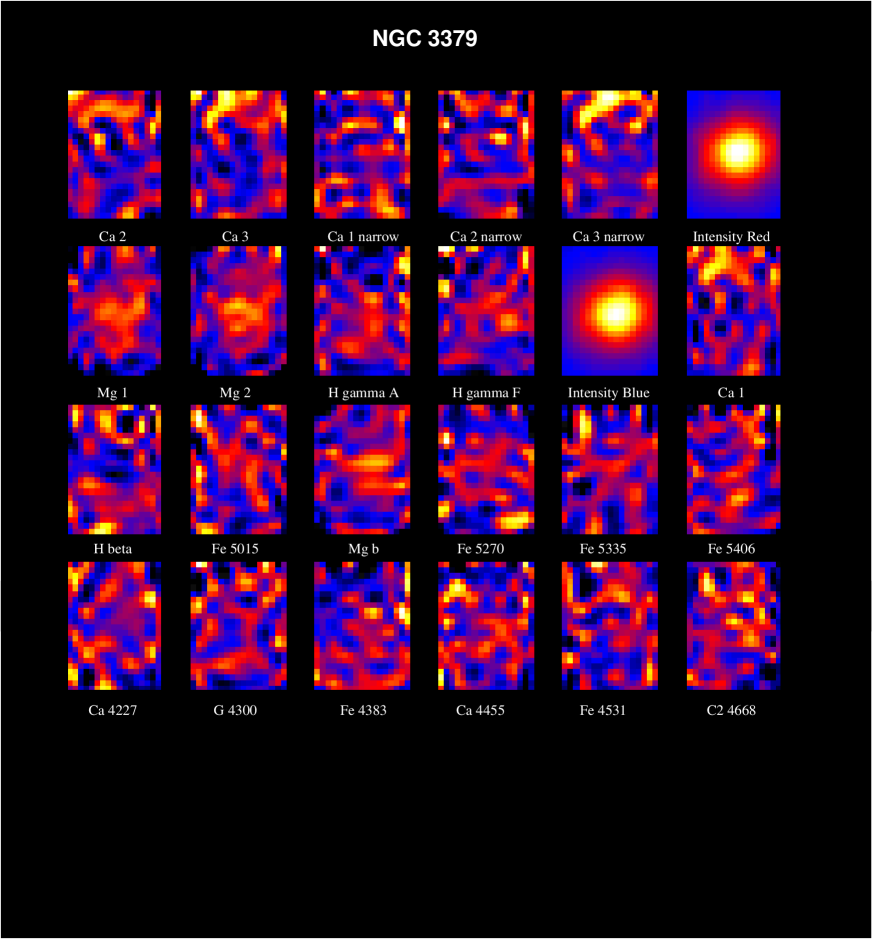
Figure 3: a: Maps of the most important line indices in blue and red for NGC 3379. The maps have been scaled in such a way that pixels that are more than 2 $\sigma$ fainter than the mean value of a map are black, while those more than 2 $\sigma$ brighter are white. If there is very little structure in a map, it will look noisier than in a case where the dynamic range in the map is large. The size of the map is 8.2^′′ $\times$ 11.0^′′

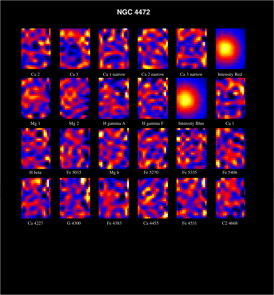
Figure 3: b: Maps of the most important line indices in blue and red for NGC 4472.

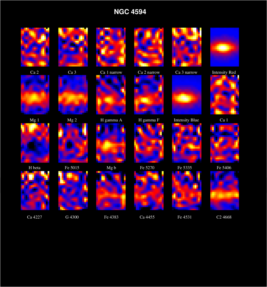
Figure 3: c: Maps of the most important line indices in blue and red for NGC 4594.

4 Comparison with the Literature

4.1 Continuum images

The first test we applied was to reconstruct the continuum images in red and blue, fit ellipses to these images, and compare them with recent HST archive images. The spectra were collapsed in the red between 8427 and 8761 ${\rm\AA}$, and in the blue between 4236 and 5643 ${\rm\AA}$. On the reconstructed images (see Fig. 3) ellipses were fit using Galphot (see Jørgensen et al. 1992). In Fig. 4 we show the blue surface brightness profiles, normalized in the center, of the three galaxies, and the profiles of the ellipticity (1-$b\over{a}$), and the major axis position angle. Also shown are profiles determined on recent HST-WFPC2 images in V (F555W), convolved to a seeing of 1.2” (FWHM). Plotted on the abscissa is $\sqrt{{\rm major}\times{\rm minor~{}axis~{}radius}}$, while the surface brightness profiles are scaled by an arbitrary number. The reconstructed images, together with the convolved HST frames, are shown in Figure 5.

Figure 4: a: Normalized blue surface brightness profiles compared to HST profiles in V, convolved to a seeing of 1.2” FWHM. Filled symbols indicate HST data; open symbols data from this paper. b: Ellipticity profiles. For clarity 0.1 has been added to the ellipticities of NGC 3379. c: Position Angle profiles. Arbitrary offsets have been applied to the HST position angle zeropoints.

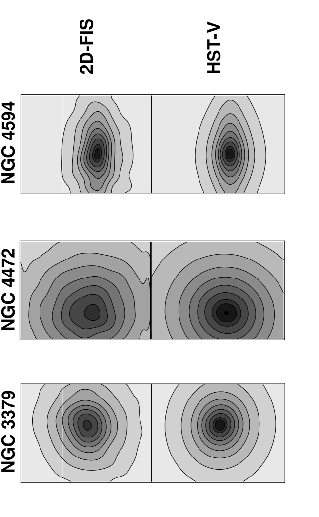
Figure 5: Comparison of our reconstructed continuum images in the blue with HST V-band images, convolved to a seeing of 1.2”. The intensities of both images have been scaled in the outer parts. Isophote levels are 0.2,0.3,0.4,0.5,0.6,0.7,0.8,0.9,0.95 and 1.00 times the maximum of the HST images. The size of the images is 8.2^′′ $\times$ 11.0^′′, the same as Fig. 3.

The agreement between the continuum images and the convolved HST V-band images is good. Their slope can be seen to be slightly shallower, which is what one expect from colour gradients, since the effective wavelength of our images is somewhat bluer than 5550 ${\rm\AA}$. The fact that the ellipticity profiles beyond 3” start diverging is due to the fact that here not the whole ellipse in included in our 2D-FIS images. Agreement in the red is not as good as in the blue, but still good. We conclude that the good agreement between our photometry and HST shows that stray light is not a problem in the analysis of our spectra.

4.2 Comparison with long-slit spectra

One of the main reasons why we are studying these 3 galaxies in such detail, is that accurate line strength profiles are available for most of the Lick indices from Paper II. In this paper the major axis of NGC 3379 and NGC 4472, and the minor axis of NGC 4594 were observed with the same spectrograph, ISIS, on the WHT, but using its regular long-slit mode. The seeing of those observations was not as good as for this paper - their effective seeing was about 2.5” - 3”. The spectra of Paper II were calibrated onto the Lick system and corrected for velocity dispersion in the same way as was done for the data in the current paper. For the comparison we turned the images of NGC 4472, NGC 3379 and NGC4594 by resp. -10, 75 and 0^o, and then extracted the line strength profiles in a column of width 1” through the center. The comparison is given in Fig. 6. In general the comparison is good, although some comments have to be made. The errorbars in the upper right corner take into the account the fiber-to-fiber errors and the error made by converting to the Lick system. One can see that most of the discrepancies can be explained by this error. One also can see that the seeing for our observations was much better - this is clear from e.g. H$\beta$, Mg₂ and Mg$b$ for the Sombrero galaxy, where the inner disk is now much better resolved. H_β and Fe 5015 in the center of the Sombrero galaxy are lower than elsewhere, because of contamination by emission; in case of the Fe 5015 line by the [OIII] line at 5007${\rm\AA}$. Agreement for well-studied indices, like $<$Fe$>$ and Mg₂ is excellent. Apart from these differences there appear to be some small global offsets, in Ca 4227, and maybe somewhat in the G-band. Our Ca 4227 is now in better agreement with the models of e.g. Worthey et al. (1994) than the data of Paper II, but the line strength is still not as large as one would expect (see Paper II).

Sometimes small ’jumps’ are seen in our index-profiles, like e.g. at -5” for the Sombrero galaxy, due to the problems described in Chapter 3. Apart from these, our index profiles are as good as most currently available profiles in the literature.

Figure 6: Comparison of our blue indices (filled symbols) with the long-slit spectra of Paper II (open symbols).

Figure 6: Comparison of our blue indices (filled symbols) with the long-slit spectra of Paper II (open symbols).

Figure 6: Comparison of our blue indices (filled symbols) with the long-slit spectra of Paper II (open symbols). The profiles corrected for [NII] emission are indicated by asteriscs.

4.3 Comparison with TIGER

The only observations of a similar kind available in the literature are those taken with TIGER, an instrument built in Lyon (Bacon et al. 1995). Tiger uses multilenslets, and compared to our current observations has a better sampling, but a much smaller wavelength range. Two detailed two-dimensional studies of the stars have been published (Emsellem et al. (1996) & Bacon et al. (1994)), of which the first deals with the Sombrero galaxy. The agreement with Emsellem’s figures 8 and 9 is good. In our study the same kinematic features are found. Although we will make a more detailed comparison in a next paper (Prada et al., in preparation), we show here that the radial velocitiy and the velocity dispersion along the major axis agree within 10 km/s (Fig. 7). In Emsellem et al. (1996) a comparison is made with Kormendy et al. (1988), which also is satisfactory.

Figure 7: Major axis cuts of radial velocity and velocity dispersion of the Sombrero galaxy, from the blue datacubes. See Emsellem et al. (1996) for a comparison with TIGER data.

To compare our Mg$b$ image with Emsellem et al. (1996)’s image, we first corrected it for emission lines. As explained in Goudfrooij & Emsellem (1996) one of the wings of this line includes an emission line of [NI] at 5199 ${\rm\AA}$, which has the effect of increasing the continuum and so also the feature’s strength. This emission is relatively strong in the Sombrero (Ho et al. 1997). We used the fact that this feature is very sharp, as compared to the wide stellar features, and removed it by interpolating across it, as one does for bad pixels. The results of this operation can be seen for Mg b and Mg₂ (which is also slightly affected) in Fig.  6. The agreement between our Mg$b$ map and Fig. 18 of Emsellem et al.  is good, reproducing in both cases the inner disk, which is strong in Mg$b$, and the peak in the center.

Since the strength of the emission line drops off quickly away from the center, it is possible to obtain an emission line spectrum by taking an average spectrum at about 2-3^′′ from the center, scaling the continuum, adjusting the velocity dispersion, and subtracting it from the central spectrum. Some emission was also found in the center of NGC 3379, but much fainter, and not strong enough to detect the [NI] 5199 ${\rm\AA}$ line, and less extended.

5 Results

5.1 Radially Averaged Profiles

In this section we present radially averaged profiles of the 3 galaxies. They have been averaged on the ellipses calculated on the continuum images. We see in Fig. 8 that the profiles of the three galaxies generally lie on top of each other, showing that the three galaxies have similar stellar populations (see also Paper II). An exception is the inner region of the Sombrero galaxy, not only because of the emission lines, but also because we see large colour gradients in lines like e.g. H$\gamma$ and Mg₂. In agreement with long slit studies most indices have non-zero radial gradients. These gradients are given in Table 4. In the red the Ca T indices seem to increase somewhat going outward, consistent between the three of them.

Figure 8: a: Radially averaged line indices in the blue. See Fig. 8b for the definition of the symbols.

Figure 8: b: Radially averaged line indices in the red.

Table 4: Line strength gradients. Results are given for simple linear fits of the line strengths as a function of the logarithm of the radius, using the radially average line strength profiles. Tabulated are the fitted line strength at r_eq = 1^′′ (a) and the gradient per dex (b).

Band	NGC 3379		NGC 4472		NGC 4594
	a	b	a	b	a	b
Ca 4227	1.078	0.036	1.359	-0.028	1.303	0.067
G 4300	6.086	-0.020	5.964	-0.170	5.932	0.158
Fe 4383	5.680	-0.410	6.114	-0.739	6.308	-1.208
Ca 4455	1.887	-0.277	2.208	-0.336	1.857	-0.275
Fe 4531	3.680	-0.251	3.965	0.204	3.531	-0.558
H$\beta$	1.150	0.421	1.286	-0.040	0.613	1.064
Fe 5015	5.300	-0.394	6.295	-0.894	5.347	-0.639
Mg b	5.110	-0.600	5.175	-0.228	5.543	-1.133
Fe 5270	3.126	-0.215	3.444	-0.193	3.231	-0.243
Fe 5335	2.624	-0.364	2.660	-0.170	2.715	-0.252
Fe 5406	1.923	-0.196	2.065	-0.199	2.109	-0.275
Mg1	0.169	-0.023	0.165	-0.009	0.184	-0.055
Mg2	0.330	-0.031	0.340	-0.014	0.352	-0.060
H$\gamma$a	-6.640	0.672	-6.734	0.630	-7.508	1.924
H$\gamma$f	-2.078	0.172	-1.815	0.254	-2.475	0.950
Ca 1	1.405	0.634	1.506	0.477	1.412	0.053
Ca 2	3.287	0.710	3.725	0.276	3.221	0.537
Ca 3	2.559	1.076	2.907	1.310	2.592	0.644
CaAZ1	1.294	-0.056	0.929	0.314	0.846	-0.046
CaAZ2	2.893	0.050	2.699	0.244	2.470	0.527
CaAZ3	2.418	0.329	2.562	0.221	2.363	0.393
CaAD1	3.247	0.037	3.397	-0.279	3.070	0.234
CaAD2	2.467	0.363	2.695	0.153	2.461	0.350
CaTP1	1.812	0.060	1.778	0.039	1.694	-0.115
CaTP2	3.589	0.004	3.740	-0.209	3.453	0.162
CaTP3	2.265	0.385	2.438	0.111	2.223	0.374

5.2 Two-Dimensional Features in the line strength maps

One of the main advantages of IFS is that one can rather easily make absorption line maps, and use them to derive conclusions about galaxy formation. In this paper we have found that the inner disk of the Sombrero is very well visible in the Mg maps (Mg₁, Mg₂ and Mgb), but is almost invisible in maps of Fe and Ca indices. This is mainly due to the fact the relative noise in the Fe and Ca maps is much larger than in the Mg features. To show this, we show in Fig. 9 a diagram of Mg₂ vs. $<$Fe$>$ that includes the nuclei of some well-observed ellipticals and spirals, some models of Vazdekis et al. (1996), and the radial profile of the Sombrero galaxy (see Section 5.1). The figure has been taken from Peletier (1999). One can see that the slope of the Sombrero is very similar to that of the models, indicating that in the Sombrero Mg/Fe remains constant, although [Mg/Fe] is larger than solar. This results appears surprising at first view. A much used explanation of overabundant Mg/Fe ratios is that the enrichment of Mg is mainly due to massive stars producing SN type II, while Fe is mainly produced in SN type Ia (see e.g. Worthey et al 1992). Since the latter originate in binaries, there is a time delay of a few times 10⁸ year between star formation and release of the Fe-peak elements in those SNe type Ia. Elliptical galaxies originally were thought to form their stars on very short timescales, as opposed to disks, and for that reason ellipticals would have enhanced Mg/Fe, while Mg/Fe in disks would be around solar. In an excellent review paper Worthey (1998), summarizing the current observational status of Mg/Fe in external galaxies, shows that this explanation is probably incorrect. Although giant ellipticals clearly have supersolar Mg/Fe ratios, this does not seem to be the case for fainter ellipticals (e.g. Davies et al. 1993), whose Mg/Fe are close to what is predicted by models with solar abundance ratios. Also, for spirals the situation is not so clear any more. Jablonka et al. (1996) find that their most luminous bulges have enhanced [Mg/Fe], but fainter ones do not. Sil’chenko (1993) finds that [Mg/Fe] is solar in most bulges of other spiral galaxies, although her sample contains very few massive galaxies. Based on these and other results Worthey concludes that the data seems to indicate that [Mg/Fe] is near zero in most galaxies of all types with velocity dispersion less than about 225 km/s, and that galaxies with velocity dispersions above that values are progressively more Mg-enhanced. Peletier (1999) slightly refines this for spirals, for which the potential is not determined only by random motions, replacing the words ’velocity dispersion’ by kinetic energy, or escape velocity.

Figure 9: Literature compilation of Mg₂ vs. $\langle$Fe$\rangle$. Plotted are central values. The meaning of the symbols is as follows: open circles are bulges of spiral galaxies (morphological type 3-5) from Jablonka et al. 1996, open triangles bulges of type 0-2 from the same paper, crosses galaxies from Carollo et al. (1993), asteriscs from Fisher et al. (1996), pentagons from Davies et al. (1993), filled circles from Halliday (1998), and plusses galaxies from Kuntschner (1998). Also added are models with solar abundance ratios of Vazdekis et al. (1996). The lines represent models of constant metallicity (resp. Z=0.008, 0.02 and 0.05 from left to right), along which age increases to the right. The line with thick symbols is the radial profile of the Sombrero galaxy (see Section 5.1).

For the Sombrero galaxy the potential well is determined by both random and ordered, rotational motion ((v/$\sigma$)_cen $\sim$ 1, Emsellem et al. 1996). Both $v$ and $\sigma_{cen}$ are larger than 225 km/s, implying, as is indeed observed, that Mg/Fe has to be larger than solar. Although the central region of the Sombrero is clearly dominated by a fast rotating disk, its Mg/Fe is much more similar to the centres of other giant early-type galaxies (for which Mg/Fe $>$ 0) than to large disks, like the disk of our Galaxy. If one believes that Mg/Fe only depends on the timescales of enrichment by SN type Ia and II, the fact that the range in observed central Mg/Fe amongst giant early-type galaxies is small would then imply that the timescale on which stars formed there would be independent on whether they are in a disk or not. Although we cannot measure these timescales at present, this could sound rather implausible, and it might be much more natural to assume that Mg/Fe depends on the IMF, which in turn would be dependent on the environment through the stellar potential. At present we don’t have any direct evidence that the IMF varies in this way, but it is much easier to explain the observations in this way, as opposed to invoking differences in timescales for enrichment by SN Ia and II.

The inner disk in the Sombrero is the only two-dimensional feature that we have found in these three galaxies. This shows that the stellar populations in the central regions of NGC 3379 and NGC 4472 are to a good approximation homogeneous.

5.3 Population Synthesis

In this section we compare the measured line-strengths with the stellar population synthesis model of Paper I. This comparison is very similar to the one performed in Paper II, apart from the fact that here we have a few extra lines (H$\gamma$ and the Ca T), and that our spatial resolution here is higher. In Paper II we showed that very good fits for the three galaxies could be obtained with single-age, single-metallicity models, SSP’s. Full evolutionary models provide solutions that are very similar, with small ranges in age and metallicity. The best fits yield good agreement for all broad band optical and near infrared colors as well as for many important line indices. Problems however are encountered when fitting Fe-dominated lines and the Ca4227 features.

To be able to use the higher spatial resolution of these observations, and to avoid too much duplication with Paper II, we have analyzed the light only in an inner aperture with a diameter of 1.7$\arcsec$ centered on the galaxy center. Best-fitting model solutions were found by minimizing a merit function M of the type described in Paper II. To calculate M, for each color or line index the square of the difference between the observed and synthetic color or index is divided by the estimated observational error and then multiplied by a certain assigned weight. To assign the weight to each index we have chosen to group them by their main contributing element, and given the same global weight to each group. These groups have been defined are as follows: Balmer indices (H$\beta$, H$\gamma_{A}$, H$\gamma_{F}$), Magnesium-dominated features (Mg₁, Mg₂, Mg_b), Iron-dominated features (Fe4383, Fe4531, Fe5015, Fe5270, Fe5335, Fe5406), Calcium-dominated features (Ca4227 and the three lines of the Ca T) and other features (G, Ca4455, C₂4668). The reason why Ca4455 is not included in the Ca group is because it is mainly a blend (Worthey et al. 1994). For that reason we have always given a low weight to this line. To survey the solution space we have defined 4 weighting functions: in the first one the same weight is assigned to each of the groups as a whole. To assess the influence of each group individually three other weighting functions were defined where the weight for one group was set to 0, while the other weights remained the same. All these weight functions are summarized in Table 5.

Relative Weights used for the Merit Function
H$\beta$	1.0	1.0	1.0	1.0
H$\gamma_{A}$	1.0	1.0	1.0	1.0
H$\gamma_{F}$	1.0	1.0	1.0	1.0
Mg1	1.0	0.0	1.0	1.0
Mg2	1.0	0.0	1.0	1.0
Mgb	1.0	0.0	1.0	1.0
Fe4383	0.5	0.5	0.0	0.5
Fe4531	0.5	0.5	0.0	0.5
Fe5015	0.5	0.5	0.0	0.5
Fe5270	0.5	0.5	0.0	0.5
Fe5335	0.5	0.5	0.0	0.5
Fe5406	0.5	0.5	0.0	0.5
Ca4227	0.5	0.5	0.5	0.0
CaII(1)	0.5	0.5	0.5	0.0
CaII(2)	1.0	1.0	1.0	0.0
CaII(3)	1.0	1.0	1.0	0.0
G	1.0	1.0	1.0	1.0
Ca4455	0.25	0.25	0.25	0.25
C24668	1.0	1.0	1.0	1.0

Table 5: Four different ways of defining the weights of the Merit Function

To fit the data, we have selected the models for three metallicities: Z=0.008, Z=0.02 (solar) andZ=0.05, and interpolated the output linearly to obtain results at Z=0.014 and 0.035. The age-range of the selected models was 1 to 17 Gyr. We preferred to use the bimodal IMF defined in Paper I, which is similar to the Salpeter IMF, but has fewer stars with mass below 0.6M_⊙, since it was shown in Paper II that this IMF provides slightly better fits to precisely the three galaxies to be analyzed here. Four IMF slopes were considered: $\mu$ = 1.0, 1.3 (Salpeter), 1.7 and 2.3.

We will now discuss the fits for the galaxies individually. The best fits were obtained for NGC 4472, giving a metallicity of Z=0.05, $\mu$=2.3 (steeper than Salpeter), and a most likely age of 8 Gyr. The same solution is found for all weight-functions, except for the case in which the Mg group is neglected, in which case an optimal age of 5 Gyr is found, with the same $\mu$ and metallicity. One should realize that we are not claiming here that with the Salpeter IMF no reasonable solutions can be found for this galaxy. Using however the bimodal IMF, which appears to be more realistic, at least for our Galaxy (Kroupa et al. 1993) it appears that we need more stars around the mass where the IMF changes slope. The fits show clearly that we cannot obtain at the same time good fits for the Mg group on one hand and the Fe+Ca groups on the other hand. This is the well known problem that giant ellipticals are overabundant in Mg (see Worthey 1998 and references therein for more details). Since the current theoretical models do not allow us to change the [$\alpha$/Fe] ratio, we will only continue with the uniform weight function for which no group has been neglected. This fit is summarized in Table 6. One sees that most of the features of the Ca group are much less strong than predicted by the model, and that these differences are clearly larger than the expected observational errors. This is the case for the lines of the Ca T, as well as for the Ca 4227 line, for which we already found in Paper II that it was much lower than expected. We would like to warn the reader that the Ca T predictions are based on an stellar library (Díaz et al. 1989) which does not properly cover all the theoretical atmospheric parameters. It is reassuring that the present observational values for the two main features of the Ca T are in agreement with the observational results of Terlevich et al. (1990): while we measure a total EW of 6.5Å  they measured 6.7Å.

The results for NGC 3379 are very similar as those for NGC 4472. Independent of the weight function the best solution is found for (Z=0.05, $\mu$=2.3, age=8 Gyr), except in the case in which the Mg group is ignored, which gives the best solution for Z=0.035, $\mu$=2.3, and age=8 Gyr. The best fit with uniform weight function is also tabulated in Table 6. For this galaxy, the Ca group features are lower than predicted, similar to NGC 4472. In general the fact that the residuals in general are larger shows that the quality of the obtained global fit is considerably worse than the fit for NGC 4472.

For the central region of the Sombrero galaxy we always obtain Z=0.05, $\mu$=2.3 and age=13 Gyr for all our weight functions except for the one where we neglect the Mg group. Here the best fit is obtained for the same IMF slope, Z=0.035 and a slightly larger age (15 Gyr). It seems that possibly better fits could be obtained with even higher metallicities. This can however not be investigated because of the lack of reliable theoretical models with Z $>$ 0.05. From the tabulated values we see that most of the features of the Ca and Fe groups show residuals much larger than the observed values and that the Mg/Fe overabundance is very pronounced. Apart from this, we also see that while the two H$\gamma$ indices are fairly well matched, this is not the case for H$\beta$ which is much lower than any model prediction. From the spectra it can be seen that this is the result of emission lines ’filling in’ the absorption line, and thereby reducing its equivalent width. Overall this galaxy yielded fits that were qualitatively the worst of the three galaxies.

To summarize our main, new results from this stellar population analysis: The strengths of the lines of the Ca T are lower than expected, confirming the result of Paper II purely on the basis of the Ca 4227 line. We find that [Ca/Fe] = 0 or slightly negative. This is peculiar, since Ca is thought to come primarily from explosive and normal oxygen burning, and is expected to follow Mg in these bright galaxies. Although our models seem to indicate that Ca is underabundant with respect to Fe (a result also confirmed by García-Vargas et al. 1998), this is not certain, as explained in Idiart et al. (1997). Because of the fact that the models of Paper I, like most currently available models, assume that [Ca/Fe] and [Ca/Mg] = 0 for the input stars that are used to calculate the fitting functions, the calculated integrated Ca T index will be too large if the stars in the input library that are used are overabundant in Ca, and vice-versa. Idiart et al. have determined Ca abundances, as well as Fe and Mg abundances, for a medium-sized input library of about 100 stars, and using individual Ca/Fe ratios for those stars they calculate models with much smaller values for the equivalent widths of the Ca T than Paper I or García-Vargas et al. (1998). Using models with solar abundance ratios we find that [Ca/Fe] for our three galaxies is about solar (see Fig. 10). Therefore, in spite of the fact that the Ca is an $\alpha$-element, the Ca-dominated features do not track Mg, but the Fe-dominated group.

		NGC 4472			NGC 3379			NGC 4594
		(Z=0.05,$\mu$=2.3,Age=8Gyr)			(Z=0.05,$\mu$=2.3,Age=8Gyr)			(Z=0.05,$\mu$=2.3,Age=13Gyr)
Index	Error	Observ.	Fit	Resid.	Observ.	Fit	Resid.	Observ.	Fit	Resid.
H$\beta$	0.262	1.325	1.273	0.2	1.048	1.273	-0.9	0.374	1.014	-2.4
H$\gamma_{A}$	0.808	-6.674	-7.811	1.4	-6.747	-7.811	1.3	-7.891	-8.549	0.8
H$\gamma_{F}$	0.342	-1.771	-2.359	1.7	-2.091	-2.359	0.8	-2.638	-2.803	0.5
Mg1	0.009	0.165	0.158	0.8	0.171	0.158	1.4	0.190	0.181	1.0
Mg2	0.010	0.339	0.331	0.8	0.333	0.331	0.2	0.371	0.365	0.6
Mgb	0.195	5.160	4.719	2.3	5.159	4.719	2.3	5.141	5.015	0.7
Fe4383	0.834	6.178	7.205	-1.2	5.692	7.205	-1.8	6.470	7.704	-1.5
Fe4531	0.455	4.067	4.181	-0.3	3.764	4.181	-0.9	3.548	4.433	-2.0
Fe5015	0.566	6.315	6.430	-0.2	5.401	6.430	-1.8	3.446	6.557	-5.5
Fe5270	0.317	3.564	3.627	-0.2	3.141	3.627	-1.5	3.231	3.818	-1.9
Fe5335	0.324	2.666	3.538	-2.7	2.701	3.538	-2.6	2.757	3.730	-3.0
Fe5406	0.228	2.056	2.293	-1.0	1.991	2.293	-1.3	2.101	2.439	-1.5
Ca4227	0.220	1.333	2.072	-3.4	1.059	2.072	-4.6	1.357	2.362	-4.6
CaII(1)	0.590	1.413	1.871	-0.8	1.178	1.871	-1.2	1.510	1.862	-0.6
CaII(2)	0.581	3.629	4.496	-1.5	3.042	4.496	-2.5	3.212	4.403	-2.1
CaII(3)	0.627	2.855	3.609	-1.2	2.368	3.609	-2.0	2.894	3.440	-0.9
G	0.395	6.048	6.005	0.1	6.136	6.005	0.3	5.966	6.112	-0.4
Ca4455	0.288	2.339	2.133	0.7	1.927	2.133	-0.7	1.890	2.264	-1.3
C24668	0.831	8.737	7.811	1.1	8.318	7.811	0.6	9.578	8.227	1.6

Table 6: Fits using uniform weighting (first column in Table 5). For each galaxy we have tabulated age, metallicity and IMF slope (for a bimodal IMF). For each index we have indicated the typical observational error for our measurements, the fitted values, and the residuals divided by the typical observational error. Note that for NGC 4594 Fe 5015 and H$\beta$ are severely affected by emission lines.

Figure 10: Models of the Ca T compared with the observations in the central aperture of 1.7^′′. The drawn lines are models of Paper II, with metallicities of Z=0.008, 0.02 and 0.05, with age ranging from 1 to 17 Gyr from left to right. The dashed lines are the models of Idiart et al. (1997) and Borges et al. (1995). In the upper figure the thick dashed lines indicate models with solar [Mg/Fe], while for the thin dashed line [Mg/Fe]=0.30.

Combining the fits obtained here with those of Paper II obtained at larger radii we can get an idea of the gradients in age, metallicity and IMF slope in these galaxies. To do this we summarize in Table 7 the fits at the 3 different positions. The table shows that the metallicity is the main parameter dominating the observed gradients. Although in the central regions of these galaxies a metallicity of more than 2 times solar is required, the metallicity decreases rapidly outward (being below solar at 15$\arcsec$), except for NGC 4472, for which the gradient is shallower. In Paper II we attributed this to the fact that this galaxy has a considerably larger effective radius than the other two. The age on the other hand does not seem to vary in an appreciable way with galactocentric radius. Only for NGC 3379 we see a slight age gradient, being somewhat younger in its center. For our understanding of these gradients it would be very useful if good observations could be obtained further away from the center.

Stellar Population Fits at various radii
Galaxy	Center (Ap. 1.7$\arcsec$)	5$\arcsec$	15$\arcsec$
NGC 4472	0.05, 2.3, 8	0.04, 2.3, 10	0.03, 2.3 10
NGC 3379	0.05, 2.3, 8	0.03, 1.5, 13	0.016, 2.3 12
NGC 4594	0.05, 2.3, 13	0.03, 2.3, 11	0.016, 2.0, 10

Table 7: The best fits at three different radii, from this paper and Paper II. Tabulated are mean metallicity, IMF slope and age in Gyr.

6 Conclusions

We have observed the well-studied galaxies the Sombrero, NGC 3379 and NGC 4594. We show that excellent two-dimensional absorption line strengths and stellar kinematics can be obtained with this instrument. We have extensively compared our results with the current literature. A detailed comparison with 2D multi-lenslet TIGER-spectroscopy of the Sombrero galaxy by Emsellem et al. (1996) shows that we can measure velocities and velocity dispersions to an accuracy of 10 km/s with our current setup, or about 0.1 pixel. We reproduce well the absorption line maps presented in that paper. An in-depth comparison with long-slit spectroscopy of Paper II shows in general good agreement between absorption line strength obtained using IFS and long-slit spectroscopy. A problem in our absorption line maps is that they contain peaks at random position which are not due to photon noise but probably to continuum variations from fiber to fiber, possibly induced by residual fringing or by variations in stress.

We show that Mg/Fe is enhanced in the whole inner disk of the Sombrero galaxy. [Mg/Fe] there is larger than in the rest of the bulge. The large values of Mg/Fe in the central disk are consistent with the centres of other early-type galaxies, and not with large disks, like the disk of our Galaxy, where [Mg/Fe] $\sim$ 0. We confirm with this observation a recent result of Worthey (1998) that Mg/Fe is determined by the central kinetic energy, or escape velocity, of the stars, only, and not by the formation time scale of the stars. In galaxies with regions with large escape velocities the IMF would have to be skewed more towards high-mass stars, which then will favor SNe type II as compared to SN type Ia, so that the Mg/Fe ratio will be enhanced.

We have obtained new observations of the Ca II IR triplet in the three galaxies, and compared them with our model predictions. We find that the observations of the Ca II IR triplet are lower than expected from the models. This result is in agreement with Paper II, where we found that the Ca 4227 line strength was lower than expected. The fact that it has been assumed in the Vazdekis models (and most others) that [Ca/Fe] and [Ca/Mg] for the stars in the stellar input libraries is solar, makes it difficult for our models to determine the [Ca/Fe] ratio in our galaxies. Using however the models of Idiart et al. (1997) who have taken these abundance ratios into account for individual stars, we find that Ca approximately tracks Fe for our three galaxies.

We find that H$\gamma$ agrees well with predictions based on other lines, including H$\beta$. Because of the fact that H$\beta$ is often severely contaminated by emission lines we confirm statements by e.g. Kuntschner & Davies (1998) that H$\gamma$ is often a very good alternative to H$\beta$ when measuring e.g. ages of galaxies.

Combining the data presented in this paper with the results of Paper II we find that the radial line strength gradients in the three galaxies are predominantly gradients in metallicity, in agreement with earlier work (e.g. Davies et al. 1993).

References

- [] Armandroff, T.E. & Zinn, R., 1988, AJ, 96, 92
- [] Armandroff, T.E. & da Costa, G.S., 1991, AJ, 101, 1329
- [] Arribas, S., Mediavilla, E. & Rasilla, J.L., 1991, ApJ, 369, 260
- [] Arribas, S., Mediavilla, E., García-Lorenzo, B. & del Burgo, C., 1997, ApJ, 490, 227
- [] Bacon, R., Emsellem, E., Monnet, G. & Nieto, J.L., 1994, A&A, 281, 691
- [] Bacon, R., Adam, G., Baranne, A., et al., 1995, A&AS, 113, 347
- [] Balcells, M. & Peletier, R.F., 1994, AJ, 107, 135
- [] Bender, R., 1990, A&A, 229, 441
- [] Borges, A.C. Idiart, T.P., de Freitas Pacheco, J.A. & Thevenin, F., 1995, AJ, 110, 2408
- [] Bruzual, G. & Charlot, S., 1993, ApJ, 405, 538
- [] Carollo, C.M., Danziger, I.J. & Buson, L., 1993, MNRAS, 265, 553
- [] Carter, D., Visvanathan, M. & Pickles, A.J., ApJ, 311, 637
- [] Davies, R.L., Sadler, E.M. & Peletier, R.F., 1993, MNRAS, 262, 650
- [] Díaz, A.I., Terlevich, E. & Terlevich, R., 1989, MNRAS, 239, 325
- [] Emsellem, E., Bacon, R., Monnet, G. & Poulain, P., 1996, A&A, 312, 777
- [] Faber, S.M., Friel, E.D., Burstein, D. & Gaskell, C.M., 1985, ApJS, 57, 711
- [] Fisher, D., Franx, M., & Illingworth, G. D. 1996, ApJ, 459, 110
- [] García, A., Rasilla, J. L., Arribas, S., & Mediavilla, E. 1994, in Instrumentation in Astronomy VIII, SPIE Vol. 2198, ed. D. L. Crawford & C. R. Craine (Hawaii: SPIE), 75
- [] García-Vargas, M.L., Mollá, M. & Bressan, A., 1998, A&A, 130, 513
- [] González, J.J., 1993, PhD Thesis, Univ. of California, Santa Cruz
- [] Gorgas, J., Faber, S.M., Burstein, D., González, J.J, Courteau, S. & Prosser, C., 1993, ApJS, 86, 153
- [] Goudfrooij, P. & Emsellem, E., 1996, A&A, 306, L45
- [] Halliday, C., 1998, Ph.D. Thesis, University of Durham
- [] Ho, L.C., Filippenko, A.V. & Sargent, W.W., 1997, ApJS, 112, 315
- [] Idiart, T.P., Thevenin, F., de Freitas Pacheco, J.A., 1997, AJ, 113, 1066
- [] Jablonka, P., Martin, P. & Arimoto, N, 1996, AJ, 112, 1415
- [] Jørgensen, I., Franx, M. & Kjaergaard, P., 1992, A&AS, 95, 489
- [] Kormendy, J., 1988, ApJ, 335, 40
- [] Kroupa, P., Tout, C.A. & Gilmore, G., 1993, MNRAS, 262, 545
- [] Kuntschner, H., 1998, Ph.D. Thesis, University of Durham
- [] Kuntschner, H. & Davies, R.L., 1998, MNRAS, 295, L29
- [] Nelson, C.H. & Whittle, M., 1995, ApJS, 99, 67
- [] Peletier, R.F., 1989, PhD Thesis, Univ. of Groningen
- [] Peletier, R.F., 1996, ING Technical Note 96
- [] Peletier, R.F., 1999, in The Evolution of Galaxies on Cosmological Timescales, eds. J.E. Beckman and T.J. Mahoney, ASP Conf. Ser, in press
- [] Peletier, R.F., Davies, R.L., Illingworth, G., Davis, L. & Cawson, M., 1990, AJ, 100, 1091
- [] Rutledge, G.A., Hesser, J.E., Stetson, P.B., Mateo, M., Simard, L., Bolte, M., Friel, E.D. & Copin, Y., 1997, PASP, 109, 883
- [] Sil’chenko, O.K., 1993, AZh Pis’ma, 19, 701
- [] Sil’chenko, O.K., Vlasyuk, V.V. & Burenkov, A.N.,, 1997, A&A, 326, 941
- [] Sil’chenko, O.K., Burenkov, A.N. & Vlasyuk, V.V., 1999, AJ, 117, 826
- [] Statler, T.S., 1991, AJ, 102, 882
- [] Terlevich, E., Díaz, A.I. & Terlevich, R., 1990, MNRAS, 242, 271
- [] Vazdekis, A., Casuso, E., Peletier, R.F. & Beckman, J.E., 1996, ApJS, 106, 307 (Paper I)
- [] Vazdekis, A., Peletier, R.F., Beckman, J. & Casuso, E., 1997, ApJS, 111, 203 (Paper II)
- [] Worthey, G., 1994, ApJS, 95, 107
- [] Worthey, G., Faber, S.M., González, J.J. & Burstein, D., 1994, ApJS, 94, 687
- [] Worthey, G., Faber, S.M. & González, J.J., 1992, ApJ, 398, 69
- [] Worthey, G. & Ottaviani, D.L., 1997, ApJS, 111, 377
- [] Worthey, G., 1998, PASP, 110, 888