Improved Treatment of Cosmic Microwave Background Fluctuations Induced by a Late-decaying Massive Neutrino

Abstract

A massive neutrino which decays after recombination ($t\geq 10^{13}$ sec) into relativistic decay products produces an enhanced integrated Sachs-Wolfe effect, allowing constraints to be placed on such neutrinos from present cosmic microwave background anisotropy data. Previous treatments of this problem have approximated the decay products as an additional component of the neutrino background. This approach violates energy-momentum conservation, and we show that it leads to serious errors for some neutrino masses and lifetimes. We redo this calculation more accurately, by correctly incorporating the spatial distribution of the decay products. For low neutrino masses and long lifetimes, we obtain a much smaller distortion in the CMB fluctuation spectrum than have previous treatments. We combine these new results with a recent set of CMB data to exclude the mass and lifetime range $m_{h}>100$ eV, $\tau>10^{12}$ sec. Masses as low as 30 eV are excluded for a narrower range in lifetime.

I Introduction

Anisotropies in the cosmic microwave background (CMB) contain an enormous amount of information about the universe. Data presently available has been used[1]-[11] to constrain from two up to eight cosmological parameters. With the promise of ever more precise measurements of these anisotropies, it has become possible to envision CMB fluctuations as a tool to go beyond this minimal set and constrain other areas of physics. Recent proposed constraints include limits on Brans-Dicke theories [12], constraints on time-variation in the fine-structure constant [13, 14], tests of finite-temperature QED [15], and limits on various models for both stable[16] and unstable [17, 18, 19] massive neutrinos. All of these additional constraints, with one exception, are based on the high-precision fluctuation spectra expected from the MAP and PLANCK satellites. The sole exception is reference [18], in which Lopez et al. pointed out that the radiation from a neutrino decaying into relativistic decay products could produce such a large integrated Sachs-Wolfe (ISW) effect, that a fairly large mass-lifetime range can be ruled out from current observations. Lopez et al. argued that a neutrino with a mass greater than 10 eV and a lifetime between $10^{13}$ and $10^{17}$ sec could be ruled out. (Although this calculation assumes nothing about the nature of the decay products other than that they are relativistic, this limit is most useful when applied to decay modes into “sterile” particles such as a light neutrino and a Majoron, since other, more restrictive limits apply to photon-producing decays). Hannestad [19] showed that the MAP and PLANCK experiments should produce an even larger excluded region in the neutrino mass-lifetime plane.

In this paper, we improve on a major approximation of references [18, 19]. In these papers, the relativistic decay products were simply added to the background neutrino energy density in the program CMBFAST [20]. However, when the massive neutrinos decay, the spatial distribution of the decay products is determined by the distribution of the non-relativistic decaying particles; it is not identical to the distribution of the background massless neutrinos. In fact, the approach of references [18, 19] violates energy-momentum conservation. Although in this approach energy and momentum are explicity conserved at zeroth order (the mean), the first order perturbations violate energy-momentum conservation. This may seem like a small effect, but it actually has significant consequences for the CMB fluctuation spectrum.

In the next section, we discuss the formalism for the Sachs-Wolfe effect in the presence of neutrinos decaying after recombination. In section III, we present our results, showing the effects of correctly incorporating the spatial distribution of the decay products, and provide a simple physical explanation of these effects. In section IV, we show how our revised calculation affects the excluded region in the neutrino mass-lifetime plane, and in section V we briefly summarize our conclusions. A comparison of our new results with current data leads to the excluded region $m_{h}>100$ eV, $\tau>10^{12}$ sec, although smaller masses can also be excluded for a smaller range of $\tau$.

II The ISW Effect with an Unstable Neutrino: Formalism

To calculate the CMB fluctuations in the presence of a decaying massive neutrino, we first review the basic precepts of the pertinent linear perturbation theory. The perturbed homogeneous, isotropic FRW metric can be parametrized as

$$ds^{2}=-a(\tau)^{2}\left[d\tau^{2}(1+2\psi)-d\vec{x}^{2}(1-2\phi)\right],$$ (1)

where $a$ is the scale factor normalized to unity today and $\tau~{}$is the conformal time defined by $d\tau=dt/a$, $t$ being the proper time of a comoving observer. This particular gauge is referred to as the conformal Newtonian gauge because the behavior of the potentials ($\phi$, $\psi$) is akin, loosely speaking, to that of the Newtonian potential. These potentials determine the large scale CMB behavior. In particular, the photon temperature perturbation decomposed into its Fourier and angular modes can be shown to be [21]

$$\Delta_{\ell}(k)=\int_{0}^{\tau_{0}}d\tau\,(\dot{\phi}(k,\tau)+\dot{\psi}(k,\tau))\exp(-\kappa(\tau))j_{\ell}(k\tau_{0}-k\tau),$$ (2)

where the subscript ‘0’ refers throughout to the present time and $\kappa$ is the optical depth from the present to some conformal time $\tau~{}$in the past. For the purpose of clarity, all the sources contributing to the anisotropy from inside the last scattering surface have been set to zero in Eq. 2. The effect of the sources contributing to the anisotropy between last scattering and the present (as given in Eq. 2) is called the Integrated Sachs-Wolfe (ISW) effect. The power in the $\ell^{th}$ multipole is normally defined as $\ell(\ell+1)C_{\ell}$ with [20]

$$C_{\ell}=(4\pi)^{2}\int_{0}^{\infty}dk\,k^{2}|\Delta_{\ell}(k)|^{2}.$$ (3)

The sources mentioned in connection with the ISW effect can be varied. At any time, the modes that are important to the ISW effect correspond to those scales which are smaller than the sound horizon of the whole fluid (matter+radiation) at that time. For these modes, the potentials can decay if there is radiation pressure or if the universe expands rapidly. In models with no cosmological constant, the main contribution to the ISW effect comes from just after recombination (since radiation redshifts faster than matter). Inclusion of a cosmological constant leading to a rapid expansion of the universe late in its history would boost the power on larger scales (small $\ell$). Any other astrophysical process which contributes to the radiation content of the universe between last scattering and the present will lead to an increase in the total ISW effect. One such scenario is that of a massive particle decaying around or after last scattering. We will consider the case of a massive neutrino decaying non-relativistically into (effectively) massless particles. The details of the daughter particles turn out to be irrelevant.

To quantify the evolution of the massive neutrino density, we will consider the Boltzmann equation for its distribution. In a homogeneous and isotropic universe, the distribution of the collisionless massive neutrino decaying non-relativistically into two massless particles follows [22]

$$\frac{\partial}{\partial\tau}f^{0}_{h}(q_{h},\tau)=-\frac{a^{2}m_{h}}{t_{d}\epsilon_{h}}f^{0}_{h}(q_{h},\tau),$$ (4)

where $t_{d}$ is the mean lifetime of the neutrino, and $\epsilon_{h}$ and $q_{h}$ are the comoving energy and momentum: $\epsilon_{h}^{2}=q_{h}^{2}+m_{h}^{2}a^{2}$, and a superscript ‘0’ will be used throughout to denote unperturbed quantities. We make the following simplifications throughout our treatment: (1) neglect inverse decays, (2) neglect spontaneous emission, (3) neglect Pauli blocking factor. The solution approaches the familiar $\exp(-t/t_{d})$ behavior as the neutrino becomes non-relativistic. The evolution equation for the energy density of the unstable neutrino is the integral of Eq. 4. It reads

$$\dot{\rho}^{0}_{h}+3\frac{\dot{a}}{a}(\rho^{0}_{h}+P^{0}_{h})=-\frac{am_{h}n^{0}_{h}}{t_{d}},$$ (5)

where overdots represent differentiation with respect to conformal time. It should be noted (as it is important if the decay is not completely non-relativistic) that the right hand side contains the product of $m_{h}$ and $n^{0}_{h}$ (number density) and not $\rho^{0}_{h}$.

We now turn on the perturbations in the metric. Although the conformal Newtonian gauge is the most useful in which to understand the ISW effect, for computational purposes we will define all our variables in the synchronous gauge. Thus, we will express the integrand in Eq. 2 in terms of perturbations in the synchronous gauge. The synchronous gauge has the property that the coordinate time and the proper time of a freely falling observer coincide. All the perturbations are in the spatial part of the metric ($g_{ij}=a^{2}\delta_{ij}+a^{2}h_{ij}$) in this gauge. The perturbation $h_{ij}$ can be Fourier transformed and broken up into its trace and a traceless part as [23]

$$h_{ij}(\vec{x},\tau)=\int d^{3}k\,\frac{\exp(i\vec{k}\cdot\vec{x})}{k^{2}}\left[h(\vec{k},\tau)k_{i}k_{j}+6\eta(\vec{k},\tau)\left(k_{i}k_{j}-\frac{k^{2}}{3}\delta_{ij}\right)\right].$$ (6)

Instead of working with the conjugate momentum in the perturbed space-time, we will use $q_{h}$ and $\epsilon_{h}$ as defined above [24] and in keeping with that, we will write out the perturbed massive neutrino distribution as

$$f_{h}(\vec{x},\vec{q}_{h},\tau)=f^{0}_{h}(q_{h},\tau)\left[1+\Psi_{h}(\vec{x},\vec{q}_{h},\tau)\right]\,.$$ (7)

Due to the fact that the decay term is linear in $f_{h}$, the form of the equation for the evolution of $\Psi_{h}$ is identical to that of the stable massive neutrino but with $f^{0}_{h}$ now given by Eq. 4. The stable massive neutrino case has been clearly worked out in Ref. [23].

The decay radiation rises exponentially from being negligible in the past to some maximum value at $\tau\sim\tau_{d}$ and then drops off as $a^{-4}$ like normal radiation. It is more informative therefore to follow the quantity $r_{rd}=\rho^{0}_{rd}/\rho^{0}_{\nu}$ where ‘rd’ denotes the decay radiation and $\rho_{\nu}^{0}$ is the cosmological density in a massless neutrino. The evolution equation for $r_{rd}$ is

$$\dot{r}_{rd}=\frac{m_{h}n^{0}_{h}}{\rho^{0}_{\nu}}\frac{a}{t_{d}}.$$ (8)

The treatment of the perturbations in the decay radiation will be analogous to that of the massless neutrino as worked out in Ref. [23]. To evolve the perturbations in the decay radiation, we will integrate out the momentum dependence in the distribution function by defining (in Fourier space)

$$F_{rd}(\vec{k},\hat{n},\tau)=\frac{\int dq\,q^{3}f^{0}_{rd}(q,\tau)\Psi_{rd}(\vec{k},q,\hat{n},\tau)}{\int dq\,q^{3}f^{0}_{rd}(q,\tau)}\;r_{rd},$$ (9)

where $\vec{q}=q\hat{n}$ and $\Psi_{rd}$ is defined analagously to Eq. 7. The equation governing the evolution of $F_{rd}$ can be worked out to give

$$\dot{F}_{rd}+ik\mu F_{rd}+4\left(\frac{\dot{h}}{6}+\frac{\dot{h}+6\dot{\eta}}{3}P_{2}(\mu)\right)r_{rd} = \dot{r}_{rd}\left(N_{0}-3iN_{1}P_{1}(\mu)-\frac{2}{3}N_{2}P_{2}(\mu)+\ldots\right),$$ (10)

$$N_{0}(k,\tau) = \frac{\int dq_{h}\,q_{h}^{2}f^{0}_{h}(q_{h},\tau)\Psi_{h}(k,q_{h},\tau)\left(1-\frac{8}{3}\left(\frac{q_{h}}{am_{h}}\right)^{2}+\ldots\right)}{\int dq_{h}\,q_{h}^{2}f^{0}_{h}(q_{h},\tau)},$$ (11)

where $\mu=\hat{k}\cdot\hat{n}$ and $P_{n}(\mu)$ are the Legendre polynomials of order $n$. The series of terms in these equations arises because the perturbed quantities depend on the direction of momentum and to get the contribution to a daughter particle with momentum $\vec{q}$, we need to integrate over all possible $\vec{q}_{h}$. Thus Eq. 10 depends on both $\mu$ and $\vec{q}\cdot\vec{q}_{h}$. The situation simplifies enormously for non-relativistic decays because each term $N_{p}$, which contributes to the $p^{th}$ multipole progressively, is of ${\cal O}(\langle q^{p}_{h}\rangle/a^{p}m^{p}_{h})$ or higher. In Eqs. 10 and 11, the series has been truncated by only keeping terms up to ${\cal O}(q^{2}_{h}/a^{2}m^{2}_{h})$ in the integrand. Similar equations for the evolution of perturbations in the decay radiation can be found in references [25], [27]. Apart from $N_{0}$, the terms on the right-hand side of Eq. (10) are completely negligible for non-relativistic decays.

The use of Eq. 10 is our only difference from the treatment in ref. [18]. In the latter paper, the relativistic decay products were simply added to the neutrino background in CMBFAST. This is equivalent to setting the right hand side of Eq. 10 to zero. Since the perturbations in the decay products are determined by the perturbations in both the metric and the decaying massive particles, they are correctly described by Eq. 10. Although this may seem like a minor difference, it produces very large effects, as we now show.

III The ISW Effect with an Unstable Neutrino: Results

The formalism outlined above for the evolution of an unstable neutrino and its decay products was integrated into the CMBFAST code [20]. We investigated a range of masses from 10 eV to $10^{4}$ eV and lifetimes from $10^{12}$ to $10^{18}$ seconds. The underlying cosmology was taken to be a standard ($\Omega=1$) CDM model with $h=0.5$ (with $H_{0}=100h$ km sec^-1 Mpc^-1); baryon density $\Omega_{B}h^{2}=.02$ and scale invariant isentropic initial conditions (the same model was used in ref. [18]). Our results are shown in Fig. 1 for several masses and lifetimes, along with the results obtained by simply adding the decay products to the relativistic background. As pointed out in Ref. [18] there is indeed an enhancement in the spectra at relatively large scales due to the ISW effect produced by the decaying neutrino. We will see in section IV that for many values of neutrino mass and lifetime, the spectrum produced is far from that observed today, and therefore a large region of parameter space is ruled out due to this effect.

FIG. 1.: The spectrum of CMB fluctuations for a standard CDM model ($\Omega_{b}=0.08$, $h=0.5$) in the presence of a decaying neutrino with the indicated mass and lifetime (solid curve). Shown for comparison is the spectrum obtained in Ref. [18] where the decay products were added to the background neutrinos (dashed curve). The dotted curve gives the fluctuation spectrum in the absence of a decaying neutrino.

The location of this ISW induced bump is determined by the lifetime of the neutrino. For lifetimes shorter than the age of the universe, inhomogeneities on scales $k$ project onto angular scales $\ell\sim k\tau_{0}$ where $\tau_{0}$ is the conformal time today, and we assume a flat universe. The potentials vary in time (and hence cause the ISW effect) most significantly at the time of decays on scales of order the sound horizon: $k_{sh}^{2}\simeq 3/(4\tau_{d}^{2}w)$ where $w=P/\rho$. Therefore, the bump in the spectrum is produced at $\ell\sim k_{sh}\tau_{0}\simeq(\tau_{0}/\tau_{d})(4w/3)^{-1/2}$. At these late times, the dominant contribution to $w$ comes from the decay radiation; hence $w\simeq\Omega_{rd}/3$ where $\Omega_{rd}$ is the fraction of critical density in decay radiation. Therefore, the ISW bump should be roughly at

$$\ell_{ISW}\simeq\frac{\tau_{0}}{\tau_{d}}\,\sqrt{\frac{9}{4\Omega_{rd}(\tau_{d})}}\,.$$ (12)

For a matter dominated universe the conformal time and time are related as follows: $\tau\propto t^{1/3}$. For a $m_{h}=10$ eV, $t_{d}=10^{15}$ sec neutrino, $\Omega_{rd}\simeq 0.15$ and $\tau_{0}/\tau_{d}\simeq(4\times 10^{17}\,\rm{sec}/10^{15}\,\rm{sec})^{1/3}\simeq 7.4$. Therefore, in this case we expect $\ell_{ISW}\simeq 29$. The actual peak occurs at a larger value of $l$, due to entropy fluctuations which decrease $w$, thereby increasing $k_{sh}$ and, finally, $\ell_{ISW}$.

Notice from Figure 1 that we find quantitative disagreement with the results of Lopez et al. [18] (dashed curves). The new results show that a more accurate treatment of the spatial distribution of the decay products produces a surprisingly large change in the CMB fluctuation spectrum compared to the results of reference [18]. This difference is larger for smaller masses as can be seen in the figure.

At least for low masses, the most obvious difference between the the old and new spectra is the smaller size of the ISW effect for the new case. This difference has a physical explanation: by not properly treating the perturbations in the decay radiation we overestimate an important source of the potential decays that drive the ISW effect. To see this we first expand the Boltzmann equation for decay radiation perturbations, Eq. 9, in multipole moments, $F_{rd}=\sum_{l}F_{rd,l}\,P_{l}$, to obtain the following hierarchy, shown here for $l\leq 2$:

$$\dot{\delta}_{rd}+\frac{2}{3}\left(\dot{h}+2\theta_{rd}\right) = \frac{\dot{r}_{rd}}{r_{rd}}\left(\delta_{h}-\delta_{rd}\right),$$ (13)

$$\dot{\theta}_{rd}-k^{2}\left(\frac{\delta_{rd}}{4}-\sigma_{rd}\right) = -\frac{\dot{r}_{rd}}{r_{rd}}\theta_{rd},$$ (14)

$$\dot{\sigma}_{rd}-\frac{2}{15}\left(2\theta_{rd}+\dot{h}+6\dot{\eta}\right) = -\frac{\dot{r}_{rd}}{r_{rd}}\sigma_{rd},$$ (15)

where $\delta_{rd}=F_{rd,0}/r_{rd}$, $\theta_{rd}=3kF_{rd,1}/4r_{rd}$ and $\sigma_{rd}=F_{rd,2}/2r_{rd}$. The treatment of Lopez et al. [18] is equivalent to neglecting the right hand sides of the equations above. This simplification breaks down near $\tau\sim\tau_{d}$, where $\dot{r}_{rd}/r_{rd}$ is not negligible.

Neglecting the $\dot{r}_{rd}/r_{rd}$ terms in the Boltzmann equations for the decay radiation perturbations results in errors in the perturbations. Let us focus on $\theta_{rd}$, which turns out to be primarily responsible for the big difference. Consider Eq. 14 for modes above the horizon at $\tau\sim\tau_{d}$, since for these modes the approximate treatment of Ref. [18] gives wrong results. For these modes the $k^{2}$ terms calculated in the approximate scheme can be shown (see Appendix) to be roughly similar to its exact value. Then the exact solution $\theta_{rd}$ is related to the approximate solution $\theta_{rd}^{a}$ by

$$\dot{\theta}_{rd}\simeq\dot{\theta}^{a}_{rd}-\frac{\dot{r}_{rd}}{r_{rd}}\,\theta_{rd}\,.$$ (16)

where the superscript here and in what follows denotes the solution to the set of equations 13-15 obtained in the approximate scheme by neglecting the feedback terms on the right hand side. The exact solution for $\theta_{rd}$ is therefore much smaller than the approximate one. Examples for several different modes are shown in Figure 2.

FIG. 2.: The difference in the variable $\theta_{rd}$ (dipole of the decay-produced radiation) between the correct and the approximate treatment in Ref. [18] is plotted for different modes: $k^{-1}=2.8\times 10^{4}$ Mpc (solid curve), $1.4\times 10^{3}$ Mpc (dotted curve), 73 Mpc (dot-dashed curve) and 23 Mpc (dashed curve).

These large overestimates of $\theta_{rd}$ lead to correspondingly large overestimates of the ISW effect and are primarily responsible for the differences between our spectra and those generated in Ref. [18]. The Appendix demonstrates precisely how the perturbations in the decay-produced radiation affect the potentials that govern the ISW effect, and how treating the decay products as identical to the massless neutrinos violates energy-momentum conservation. The bottom line is that the ISW effect depends significantly on the behavior of $\theta_{rd}$ and inaccuracies in it lead directly to inaccuracies in the $C_{l}$’s. Why does the approximation work better for higher mass neutrinos? The ISW effect is generated during times when the universe has appreciable radiation. For low-mass neutrinos whose decay radiation never dominates the energy density, the decay radiation redshifts away relative to the matter, and is only important near $\tau\sim\tau_{d}$. Therefore, neglecting the $\dot{r}_{rd}/r_{rd}$ terms creates errors in the decay radiation perturbations at the crucial time when they are driving the ISW effect. If the neutrino is massive enough, then its decay products are important for a range of times with $\tau\gg\tau_{d}$ when the approximation is good. So the approximate treatment works better for higher-mass neutrinos, like the $m_{h}=10$ keV, $t_{d}=10^{12}$ sec case.

There are other visible differences between the anisotropy spectra generated in reference [18] and our more accurate treatment. One difference, which exacerbates the rise in power at large scales, is a drop in the small-scale ISW effect. For modes which enter the horizon when there is significant radiation, the $\delta_{h}$ term in Eq. (13) is an important source term. This increases $\delta_{rd}$ relative to $\delta_{rd}^{a}$ and since $\delta_{rd}$ is a source for the evolution of $\theta_{rd}$, it implies that $\theta_{rd}^{a}<\theta_{rd}$. Thus there is a decrease in the ISW effect at small scales in the approximate scheme of ref [18]. This is not visible for the 10 eV unstable neutrino (in Fig. 1) because of the comparatively large signature of the first peak, but it is readily apparent for the 10 keV neutrino because of the large ISW effect at small scales.

IV Comparison with current CMB data

Since the detection of anisotropies in the CMB by COBE[28], there have been dozens of observations of anisotropies on a wide variety of angular scales (refs. [29]-[40]). We now use these observations to place more accurate limits on neutrino mass and lifetime.

In ref. [18], a very rough constraint was placed on decaying neutrino models: a model was excluded if the power at $l=200$ was greater than at $l=10$. As we have noted in the previous section, a more accurate treatment of the decaying neutrinos results in a much smaller distortion in the CMB spectrum for a certain range of neutrino masses and lifetimes. However, as we will see, consideration of all the data leads to constraints which are almost as stringent as the rough contours in ref. [18].

CMB experiments typically report an estimate of the band power

$$\hat{C}_{i}={1\over 4\pi}{\sum_{l}(2l+1)W_{i,l}C_{l}\over\sum_{l}W_{i,l}/l}$$ (17)

where $W_{i,l}$ is the window function which depends on beam size and chopping strategy of experiment $i$. Each of these comes with an error bar or, in the case of correlated measurements, an error matrix $M^{-1}$. The naive way to constrain parameters in a theory then is to form

$$\chi^{2}=\sum_{i,i^{\prime}}\left(\hat{C}_{i}-C_{i}(C_{l})\right)M_{ii^{\prime}}\left(\hat{C}_{i^{\prime}}-C_{i^{\prime}}(C_{l})\right).$$ (18)

Here we have explicitly written the dependence of $C_{i}$ on the theoretical $C_{l}$’s which in turn depend on the cosmological parameters. This naive statistic is useful only if the band power errors are Gaussian. In fact, the probability distribution is typically non-Gaussian, with a large tail at the high end and a sharp rise at the low end of the distribution. In recognition of this, and guided by some compelling theoretical arguments, Bond, Jaffe, and Knox [41] proposed forming an alternative statistic:

$$\chi^{2}=\sum_{i,i^{\prime}}\left(\hat{Z}_{i}-Z_{i}(C_{l})\right)M^{Z}_{ii^{\prime}}\left(\hat{Z}_{i^{\prime}}-Z_{i^{\prime}}(C_{l})\right)$$ (19)

where

$$Z_{i}\equiv\ln\left(C_{i}+x_{i}\right)$$ (20)

with $x_{i}$ an experiment dependent quantity, determined by the noise. The covariance matrix is now

$$M^{Z}_{ij}=\left(\hat{C}_{i}+x_{i}\right)M_{ij}\left(\hat{C}_{i}+x_{i}\right).$$ (21)

Bond, Jaffe, and Knox [41] have tabulated and made available the relevant data from the experiments in refs. [28]-[40]. We use this information and formalism to constrain the mass and lifetime of unstable neutrinos.

The $\chi^{2}$ in eq. 19 depends on the parameters of the cosmological model. In principle, it would be nice to allow as many parameters as possible to vary in addition to the mass and lifetime of the neutrino. This must be balanced against the constraints imposed by non-negligible time needed to run the modified version of CMBFAST. Our strategy is to vary the mass and lifetime of the neutrino; the overall normalization of the $C_{l}$’s; the primordial spectral index (equal to one for Harrison-Zel’dovich fluctuations); and the calibration of each experiment. For the other cosmological parameters, we make “conservative” choices. That is, we choose values likely to make the power on small scales $(l\sim 200)$ as large as possible compared with the power on large scales. This acts against the effect of the decaying neutrino, which boosts up power on large scales, and therefore leads to more conservative limits. At each point in $(m,\tau)$ space, we use a Levenberg-Marquardt algorithm (see e.g. [43, 44]) to find the values of normalization, spectral index, and calibration which minimize the $\chi^{2}$ defined in Eq. 19. The contours in Fig. 3 show these best fit $\chi^{2}$ in the $(m,\tau)$ plane.

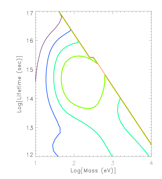
FIG. 3.: Contours of $\chi^{2}$ in neutrino mass/lifetime plane in $1-\sigma$ intervals. Inner contour is ruled out at $4\sigma$; outermost contour is $1\sigma$. The upper right part of the figure leads to $\Omega>1$ (the jaggedness at $\log\tau\simeq 15.5$ reflects the grid size used to explore the parameter space). Here $h=0.5;\Omega_{B}=0.08$.

Figure 3 shows the constraints on the neutrino mass and lifetime for a Hubble constant $h=0.5$ and $\Omega_{B}h^{2}=.02$ in a flat ($\Omega=1$) matter dominated ($\Omega_{\Lambda}=0$) universe. The high baryon content is above the favored value of Tytler and Burles [42] and serves to raise the power on small scales. Masses greater than $100$ eV are ruled out for almost all lifetimes we have explored ($\tau>10^{12}$ sec). For lifetimes between $10^{14}$ and $10^{15}$ sec, masses as low as $30$ eV are excluded at the two-sigma level. These results are similar to those of ref. [18], but more reliable because of the improvements in the calculated spectra and the more careful treatment of the data.

We checked that the contours for a different set of $(h,\Omega_{b})$ were similar to the contours in Fig 3. Fig. 4 shows the results for a cosmological constant-dominated universe. Again, a sizable region is ruled out, reflecting the robustness of the constraint.

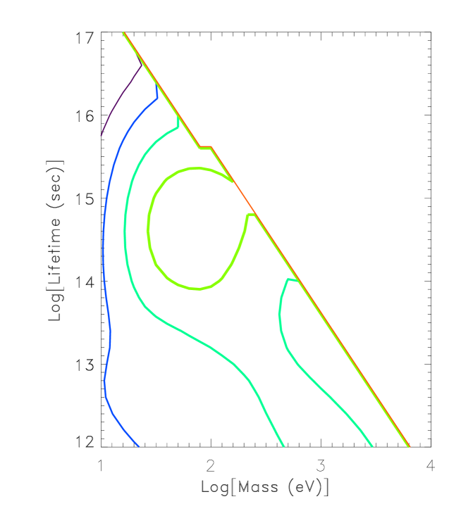
FIG. 4.: Same as Fig. 3, but now $\Omega_{\Lambda}=0.7,\Omega_{total}=1$.

Hannestad [19] performed a similar calculation, using future CMB experiments to rule out decaying neutrino models, but he used the same approximation as in reference [18]; the decay products were added into the background neutrino density. We expect that his excluded-region contours for low masses should shrink since ISW effect is the main discriminator for these masses.

It has been noted that the decay products from a very massive neutrino could keep the universe substantially populated with radiation or even radiation-dominated for most of its history. The presence of radiation has the effect of stopping the growth of density perturbations, which in a matter-dominated universe would grow as $\delta\sim a$. Since these density perturbations should (eventually) collapse into the structure we see today, it is clear that structure formation arguments can also provide constraints on the neutrino mass and lifetime. Very coarse constraints on the radiation density can placed by requiring that the scales relevant to structure formation are able to grow sufficiently (assuming of course, we know the initial perturbations), as is done in Ref. [26]. In fact, for a scale-invariant initial spectrum, the structure formation arguments of Ref. [26] also rule out a region at the bottom-right of our excluded region. A more detailed analysis yields more stringent constraints [27]. In light of this, it is important to understand that the constraints from CMB are most useful for low masses, i.e., for massive decaying neutrinos which do not affect the late-time growth of the density perturbations appreciably. Future experiments (MAP and PLANCK) have the potential to constrain neutrino masses as low as 1 eV and maybe even lower [19]. In the end, CMB and large scale structure constraints on massive decaying neutrinos both overlap and complement each other.

V Conclusions

Our results indicate that for calculations involving the effects of decaying particles on CMB fluctuations, exact conservation of energy-momentum (not just conservation of the mean energy-momentum) is crucial. When perturbations in the decay products are correctly treated as being determined by the perturbations in both the metric and the decaying massive particle, energy and momentum of the massive particle plus its decay products are conserved. The result is a much smaller change (when an unstable neutrino is added) in the CMB fluctuation spectrum than was noted in ref. [18]. However, by using a comparison with current data, rather than a simple constraint on $C_{200}/C_{10}$, we have been able to obtain an excluded region only slightly less restrictive than that obtained in ref. [18]. This excluded region will grow as more data becomes available, culminating potentially in very restrictive limits from MAP and PLANCK [19]. Our results, of course, can be generalized to arbitrary decaying particles.

The CMB spectra used in this work were generated with a modified version of CMBFAST [20]. We thank Lloyd Knox for providing the data used to generate the constraints in section IV. This work was supported by the DOE and the NASA grant NAG 5-7092 at Fermilab and by the DOE grant DE-FG02-91ER40690 at Ohio State.

A Source of Decaying Potentials

Here we show that the ISW effect in the decaying neutrino model is primarily driven by the dipole of the decay-produced radiation, $\theta_{rd}$. The ISW effect is driven by time changes to the potentials (eq. 2), which are determined from Einstein’s equations. In synchronous gauge, the source of these time changes is

$$\dot{\phi}+\dot{\psi}=t_{1}+t_{2}+t_{3}+t_{4}\,,$$ (A1)

where
$\displaystyle t_{1}$ $\displaystyle=$ $\displaystyle\left[2+\frac{3}{k^{2}}\left(\frac{\dot{a}}{a}\right)^{2}(5+3w)\right]\dot{\eta}\,,$ $\displaystyle t_{3}$ $\displaystyle=$ $\displaystyle-2\frac{\dot{a}}{a}\eta\,,$ $\displaystyle t_{2}$ $\displaystyle=$ $\displaystyle\frac{1}{2k^{2}}\left(\frac{\dot{a}}{a}\right)^{2}(5+3w)\dot{h}\,,$ $\displaystyle t_{4}$ $\displaystyle=$ $\displaystyle\frac{3}{k^{2}}\left(2\frac{\dot{a}}{a}D_{\sigma}-\dot{D}_{\sigma}\right)\,.$
The quantity $D_{\sigma}$ is related to the anisotropic stress of the fluid: $D_{\sigma}=-(3/2)\,(\dot{a}/a)^{2}\,(1+w)\,\sigma$, where $w=P/\rho$ is the equation of state of the universe. We will consider the behavior of superhorizon-scale perturbations, where $k\tau\ll 1$. We assume that the neutrinos decay well into the matter-dominated phase of the universe, and that the decay radiation never dominates the energy density of the universe, but does come to dominate the standard radiation, i.e., photons and massless neutrinos. Then the equation of state takes a simple form near neutrino decay: $w\simeq 1/3\,\Omega_{rd}$. In addition, the total fluid perturbation sources $\theta$ and $\sigma$ are dominated by the decay radiation, so that we can write $\theta\simeq 4w\,\theta_{rd}$, and $\sigma\simeq 4w\,\sigma_{rd}$. These assumptions are well motivated for $m_{h}=10$ eV, $t_{d}=10^{15}$ sec neutrinos which decay well into the matter dominated era, with $\Omega_{rd}\simeq 0.15$ at decay.

We first examine the behavior of $\dot{\phi}+\dot{\psi}~{}$in the approximation where we neglect the $\dot{r}_{rd}/r_{rd}$ terms in the Boltzmann equations for the decay radiation perturbations, i.e., we treat the decay radiation as massless neutrinos as in Lopez, et al [18]. We then consider the effect of relaxing the approximation and calculating the decay radiation perturbations correctly. We denote the use of the Lopez et al. [18] approximation in all quantities by the superscript-$a$.

The potentials do not decay in a completely matter-dominated universe; $\dot{\phi}+\dot{\psi}$ is sourced by the decay radiation and is therefore first order in $w$. The term $t^{a}_{4}$ is directly related to $\sigma$ and so is of order $w$. The linearized Einstein equations imply that $\dot{\eta}\propto\theta\propto w\,\theta_{rd}$, so that $t^{a}_{1}$ is also of order $w$. However, $t^{a}_{2}$ and $t^{a}_{3}$ are each zeroth order in $w$, so their sum must cancel to lowest order. Using the linearized Einstein equations and the continuity equation we find that

$$t^{a}_{2}+t^{a}_{3}\simeq 8\frac{w\eta}{\tau}\,,$$ (A3)

demonstrating the required cancellation. In our approximation, the decay radiation perturbations can be calculated from the Boltzmann equation for massless neutrinos, which admit analytic solutions for the superhorizon modes of $\theta^{a}_{rd}$ and $\sigma^{a}_{rd}$. Using these solutions, it can be shown that

$$t^{a}_{1}\simeq-29\frac{w\eta}{\tau}\,,\;t^{a}_{4}\simeq 12\frac{w\eta}{\tau}\,,$$ (A4)

so that $t^{a}_{1}$, $t^{a}_{2}+t^{a}_{3}$ and $t^{a}_{4}$ each contribute roughly comparable amounts to $\dot{\phi}+\dot{\psi}~{}$. In calculating the effect of the approximation on $\dot{\phi}+\dot{\psi}~{}$we will therefore have to separately consider each term. The quantities $D_{\sigma}$ and $\dot{\eta}$ are very much affected by the approximation, since they directly depend on the decay radiation perturbations, and the error in the decay radiation perturbations is of order the quantities themselves. This implies that $\delta\dot{\eta}\sim|\dot{\eta}|$ and $\delta D_{\sigma}\sim|D_{\sigma}|$, where $\delta x\equiv|x-x^{a}|$ is the absolute error in the variable $x$. The zeroth order quantities $\eta$ and $\dot{h}$ are much less affected by the approximation. For super-horizon modes, we do not expect $\eta$ to evolve much from its initial value, and so the error in it (determined by the error in $\dot{\eta}$) is naturally small. Following this line of reasoning, one can write

$$\delta\eta \sim \delta\dot{\eta}\,\tau\sim k^{2}\,\tau^{2}\,w\,\eta,$$ (A5)

$$\delta\dot{h} \sim k^{2}\,\tau\,\delta\eta\sim k^{4}\,\tau^{3}\,w\,\eta.$$ (A6)

Using these relations we find that

$$\delta t_{1}\sim\frac{w\,\eta}{\tau}\,,\;\delta t_{2}\sim(k\tau)^{2}\frac{w\,\eta}{\tau}\,,\;\delta t_{3}\sim(k\tau)^{2}\frac{w\,\eta}{\tau}\,,\;\delta t_{4}\sim\frac{w\,\eta}{\tau}\,,$$ (A7)

which makes it clear that for superhorizon modes, the errors in $t_{1}$ and $t_{4}$ dominate the error in $\dot{\phi}+\dot{\psi}~{}$. Numerically it is seen that the error in $t_{1}$ is the most important.

We can see why the error in $t_{1}$ is the most important in a simple way. The dominant source term (see eq. 14) for $\dot{\theta}^{a}_{rd}$ is $\delta_{rd}^{a}$. Now $\dot{\delta}_{rd}$ and $\dot{\delta}^{a}_{rd}$ differ only by the terms on the right-hand side of eq. 13 (since $\dot{h}$ is not much affected by the approximation and $\theta_{rd}\ll\dot{h}$ for super-horizon modes). But the right-hand side of eq. 13 contains the difference of $\delta_{h}$ and $\delta_{rd}$, and hence the fractional error in $\delta_{rd}$ is expected to be much smaller relative to that in $\theta_{rd}$ or $\sigma_{rd}$. So we can assume that $\delta_{rd}$ and $\delta_{rd}^{a}$ are roughly the same for the purpose of estimating the errors in $\theta_{rd}$ and $\sigma_{rd}$ in the approximate scheme. Therefore, for super-horizon modes (at $\tau\sim\tau_{d}$), we can write to a good approximation

$$\dot{\theta}_{rd}\simeq\dot{\theta}^{a}_{rd}-\frac{\dot{r}_{rd}}{r_{rd}}\,\theta_{rd}\quad\mbox{and}\quad\dot{\sigma}_{rd}\simeq\dot{\sigma}^{a}_{rd}-\frac{\dot{r}_{rd}}{r_{rd}}\,\sigma_{rd}\,.$$ (A8)

From this equation, we can gauge that the fractional errors in $\theta_{rd}$ and $\sigma_{rd}$ are roughly the same, and close to $-\tau\,\dot{r}_{rd}/r_{rd}$. But since the coefficient for $t_{4}$ in $\dot{\phi}+\dot{\psi}~{}$is much less than that for $t_{1}$ (see eq. A4), we expect that the error in $t_{1}$ dominates which implies that $\delta(\dot{\phi}+\dot{\psi})\propto\dot{\eta}\propto\theta_{rd}$. From eq. A8 we have that $\theta^{a}_{rd}>\theta_{rd}$ for super-horizon modes at $\tau\sim\tau_{d}$. Therefore for these modes,

$$\left|{\dot{\phi}}^{a}+{\dot{\psi}}^{a}\right|>\left|\dot{\phi}+\dot{\psi}\right|\,.$$ (A9)

This is the reason for the dramatic rise in power at large scales when we neglect the decay terms in the decay radiation Boltzmann equations.

Merely adding the decay radiation to the massless neutrino background causes large errors in the ISW effect. However, there exists a method of calculation that yields good results without introducing a separate Boltzmann hierarchy for the decay radiation. Since this method might be helpful for other late time processes which affect the CMB spectrum, and since it demonstrates that we really have isolated the source of our disagreement with Lopez et al. [18], we present it here.

The fix can be accomplished by explicitly evolving $\alpha=1/(2k^{2})(\dot{h}+6\dot{\eta})$, a quantity that contains the problematic $\dot{\eta}$, within CMBFAST in the following differential equation:

$$\dot{\alpha}+2\frac{\dot{a}}{a}\alpha=\eta-\frac{9}{2k^{2}}\,\left(\frac{\dot{a}}{a}\right)^{2}\,(1+w)\,\sigma$$ (A10)

The dominant quantity on the right-hand side is $\eta$, which is quite unaffected by the approximation (recall that $\delta\eta\sim k^{2}\,\tau^{2}\,w\,\eta$. In contrast, when $\alpha$ is set by the equation (the default in CMBFAST),

$$\alpha=\frac{a}{\dot{a}}\,\eta+\frac{3}{2k^{2}}\,\frac{\dot{a}}{a}\,\delta+\frac{9}{2k^{4}}\,\left(\frac{\dot{a}}{a}\right)^{2}\,(1+w)\,\theta\,,$$ (A11)

the $\theta$ term is important, and inaccuracies in the large scale behavior are generated. The condition that $\dot{\alpha}$ given by Eq. (A10) should match that obtained from Eq. (A11) is conservation of momentum for the massive neutrino and its decay products. In the approximate scheme, the unperturbed quantities for the decay radiation are calculated correctly while the perturbations in it are set equal to that of the massless neutrino. This violates the energy-momentum conservation conditions for the system of the massive neutrino plus its decay products, and this is the reason behind the fact that different combinations of the Einstein equations lead to different potential decay rates. It may be noted that the CMBFAST code [20] used to calculate the fluctuation spectrum implicitly assumes energy-momentum conservation. When this condition is violated, the code cannot produce internally consistent results. In Fig. 5, we have plotted the result of using Eq. A10 (in place of Eq. A11) with the approximate scheme and as expected, good agreement with the actual curves is obtained. This exercise clearly shows that it is important to check for energy-momentum conservation when using approximate methods to model any part of the energy-momentum tensor.

FIG. 5.: The spectrum of CMB fluctuations for a standard CDM model ($\Omega_{b}=0.08$, $h=0.5$) in the presence of a decaying neutrino with the indicated mass and lifetime (solid curve). The dashed curve is the spectrum obtained when the decay products are added to the background neutrinos and $\alpha$ is evolved as an explicit differential equation instead of being fixed as in the standard CMBFAST code. The dotted curve gives the fluctuation spectrum in the absence of a decaying neutrino.

REFERENCES

- [1] E. F. Bunn & M. White, ApJ480, 6 (1997).
- [2] P. de Bernardis et al., ApJ480, 1 (1997).
- [3] C. H. Lineweaver, ApJ505, L69 (1998).
- [4] S. Hancock et al., MNRAS 294, L1 (1998).
- [5] J. Lesgourgues et al., astro-ph/9807019 (1998).
- [6] J. Bartlett et al., astro-ph/9804158 (1998).
- [7] J. R. Bond & A. H. Jaffe, astro-ph/98089043 (1998).
- [8] A. M. Webster, ApJ509, L65 (1998).
- [9] M. White, ApJ506, 485 (1998).
- [10] B. Ratra et al., ApJ517, 549 (1999).
- [11] M. Tegmark, ApJ514, L69 (1999).
- [12] A. R. Liddle, A. Mazumdar & J. D. Barrow, Phys. Rev. D58, 027302 (1998); X. Chen & M. Kamionkowski, astro-ph/9905368 (1999).
- [13] S. Hannestad, astro-ph/9810102 (1998).
- [14] M. Kaplinghat, R.J. Scherrer & M.S. Turner, astro-ph/9810133 (1998).
- [15] R. E. Lopez, S. Dodelson, A. Heckler & M. S. Turner, Phys. Rev. Lett.82, 3952 (1999).
- [16] S. Dodelson, E.I. Gates, & A. Stebbins, ApJ467, 10 (1996); J.R. Bond, G. Efstathiou & M. Tegmark, MNRAS 291, L33 (1997).
- [17] M. White, G. Gelmini & J. Silk, Phys. Rev. D51, 2669 (1995); S. Hannestad, Phys. Lett. B431, 363 (1998); J.A. Adams, S. Sarkar & D.W. Sciama, MNRAS 301, 210 (1998); S. A. Bonometto & E. Pierpaoli, astro-ph/9806035 (1998); E. Pierpaoli & S. A. Bonometto, astro-ph/9806037 (1998).
- [18] R. E. Lopez, S. Dodelson, R. J. Scherrer & M. S. Turner, Phys. Rev. Lett.81, 3075 (1998).
- [19] S. Hannestad, Phys. Rev. D59, 125020 (1999).
- [20] U. Seljak & M. Zaldarriaga, ApJ469, 437 (1996).
- [21] W. Hu & N. Sugiyama, Phys. Rev. D50, 627 (1994).
- [22] M. Kawasaki, G. Steigman & H. Kang, Nucl. Phys. B 403, 671 (1993).
- [23] C.-P. Ma & E. Bertschinger, ApJ455, 7 (1995).
- [24] J. R. Bond & A. Szalay, ApJ276, 443 (1983).
- [25] J. R. Bond & G. Efstathiou, Phys. Lett. B 265, 245 (1991).
- [26] G. Steigman & M. Turner, Nuc. Phys. B 253, 375 (1985).
- [27] S. Bharadwaj & S. K. Sethi, ApJSupp. 114, 37 (1998).
- [28] C. Bennett et al., ApJ464, L1 (1996).
- [29] K. Ganga, L. Page, E. S. Cheng & S. S. Meyer, ApJ432, L15 (1994).
- [30] S. M. Gutteriez de la Cruz et al., ApJ442, 10 (1995); S. Hancock et al., Nature 367 333 (1994); R. Watson et al., Nature 357 660 (1992).
- [31] G. S. Tucker et al., ApJ475, L73 (1997)
- [32] T. Gaier et al., ApJ398, L1 (1992); J. Schuster et al., ApJ412, L47 (1993); J. O. Gundersen et al., ApJ413, L1 (1993); J. O. Gundersen et al., ApJ443, L57 (1995).
- [33] J. Ruhl et al., ApJ453, L1 (1995); S. R. Platt et al., ApJ475 L1 (1997).
- [34] M. Devlin et al., astro-ph/9808043 (1998); T. Herbig et al., astro-ph/9808044 (1998); A. de Oliveira-Costa et al.,astro-ph/9808045 (1998).
- [35] P. Meinhold & P. Lubin, ApJ370, L11 (1989).
- [36] S. Masi et al., ApJ463, L47 (1996); P. deBernardis et al., ApJ422, L33 (1994).
- [37] A. Clapp et al., ApJ433, L57 (1994); M. J. Devlin et al., ApJ430, L1 (1994); M. A. Lim et al., ApJ469, L69 (1996).
- [38] C. B. Netterfield et al., ApJ474, 47 (1995); E. Wollack et al., ApJ476, 440 (1995).
- [39] E. Cheng et al., ApJ422, L37 (1994); E. Cheng et al., ApJ488, L59 (1997); G. W. Wilson et al., astro-ph/9902047 (1999).
- [40] P. F. S. Scott et al., ApJ461, L1 (1996); J. C. Baker et al., astro-ph/9904415 (1999).
- [41] J.R. Bond, A.H. Jaffe & L.E. Knox, astro-ph/9808264 (1998).
- [42] S. Burles & D. Tytler, astro-ph/9803071 (1998).
- [43] W. H. Press, S. A. Teukolsky, W. T. Vetterling & B. P. Flannery, Numerical Recipes (Cambridge, 1992).
- [44] S. Dodelson & L. Knox, in preparation.