Chemo–Dynamical SPH code for evolution of star forming disk galaxies.

Abstract

A new Chemo–Dynamical Smoothed Particle Hydrodynamic (CD-SPH) code is presented. The disk galaxy is described as a multi–fragmented gas and star system, embedded in a cold dark matter halo with a rigid potential field. The star formation (SF) process, SNII, SNIa and PN events, and the chemical enrichment of gas, have all been considered within the framework of the standard SPH model, which we use to describe the dynamical and chemical evolution of triaxial disk–like galaxies. It is found that such approach provides a realistic description of the process of formation, chemical and dynamical evolution of disk galaxies over a cosmological timescale.

Key words: chemical and dynamical evolution of disk galaxies – CD-SPH – star formation in SPH

1 Introduction

The dynamical and chemical evolution of galaxies is one of the most interesting and complex of problems. Naturally, galaxy formation is closely connected with the process of large–scale structure formation in the Universe.

The main role in the scenario of large–scale structure formation seems to be played by the dark matter. It is believed that the Universe was seeded at some early epoch with low density fluctuations of dark non–baryonic matter, and the evolving distribution of these dark halos provides the arena for galaxy formation. Galaxy formation itself involves collapse of baryons within potential wells of dark halos ([White & Rees 1978]). The properties of forming galaxies depend on the amount of baryonic matter that can be accumulated in such halos and the efficiency of star formation. The observational support for this galaxy formation scenario comes from the recent COBE detection of fluctuations in the microwave background (e.g.[Bennett et al. 1993]).

The investigation of galaxy formation is a highly complex subject requiring many different approaches. The formation of self–gravitating inhomogeneities of protogalactic size, the ratio of baryonic and non–baryonic matter ([Bardeen et al. 1986]; [White & Silk 1979]; [Peebles 1993]; [Dar 1995]), the origin of the protogalaxy’s initial angular momentum ([Voglis & Hiotelis 1989]; [Zurek et al. 1988]; [Eisenstein & Loeb 1995]; [Steinmetz & Bartelmann 1995]), and the protogalaxy’s collapse and its subsequent evolution are all usually considered as separate problems. Recent advances in computer technology and numerical methods have allowed detailed modeling of baryon matter dynamics in the universe dominated by collisionless dark matter and, therefore, the detailed gravitational and hydrodynamical description of galaxy formation and evolution. The most sophisticated models include radiative processes, star formation and supernova feedback (e.g.[Katz 1992]; [Steinmetz & Muller 1994]; [Friedli & Benz 1995]).

The results of numerical simulations are essentially affected by the star formation algorithm incorporated into modeling techniques. The star formation and related processes are still not well understood on either small or large spatial scales, such that the star formation algorithm by which the gas material is converted into stars can only be based on simple theoretical assumptions or on empirical observations of nearby galaxies. The other most important effect of star formation on the global evolution of a galaxy is caused by a large amount of energy released in supernova explosions and stellar winds.

Among numerous methods developed for the modeling of complex three dimensional hydrodynamic phenomena, Smoothed Particle Hydrodynamics (SPH) is one of the most popular ([Monaghan 1992]). Its Lagrangian nature allows easy combination with fast N–body algorithms, making it suitable for simultaneous description of the complex dynamics of a gas–stellar system ([Friedli & Benz 1995]). As an example of such a combination, the TREE-SPH code ([Hernquist & Katz 1989]; [Navarro & White 1993]) was successfully applied to the detailed modeling of disk galaxy mergers ([Mihos & Hernquist 1996]) and of galaxy formation and evolution ([Katz 1992]). The second good example is a GRAPE-SPH code ([Steinmetz & Muller 1994]; [Steinmetz & Muller 1995]) which was successfully used to model the evolution of disk galaxy structure and kinematics.

In recent years, there have been excellent papers concerning the complex SPH modeling of galaxy formation and evolution ([Raiteri et al. 1996]; [Carraro et al. 1997]). Our code, proposes new ”energetic” criteria for SF, and suggest a more realistic account of returned chemically enriched gas fraction via SNII, SNIa and PN events.

The simplicity and numerical efficiency of the SPH method were the main reasons why we chose this technique for the modeling of the evolution of complex, multi–fragmented triaxial protogalactic systems. We used our own modification of the hybrid N–body/SPH method ([Berczik & Kravchuk 1996]; [Berczik 1998]), which we call the chemo–dynamical SPH (CD-SPH) code.

The ”dark matter” and ”stars” are included in the standard SPH algorithm as the N–body collisionless system of particles, which can interact with the gas component only through gravitation ([Katz 1992]). The star formation process and supernova explosions are also included in the scheme as proposed by Raiteri et al.(1996), but with our own modifications.

2 The CD-SPH code

2.1 The SPH code

Continuous hydrodynamic fields in SPH are described by the interpolation functions constructed from the known values of these functions at randomly positioned particles ([Monaghan 1992]). Following Monaghan & Lattanzio (1985) we use for the kernel function $W_{ij}$ the spline expression in the form of:

$$W_{ij}=\frac{1}{\pi h^{3}}\left\{\begin{array}[]{lllll}1-\frac{3}{2}u_{ij}^{2}+\frac{3}{4}u_{ij}^{3},&\mbox{ if $0\leq u_{ij}<1$},\\ \\ \frac{1}{4}(2-u_{ij})^{3},&\mbox{ if $1\leq u_{ij}<2$},\\ \\ 0,&\mbox{ otherwise }.\\ \end{array}\right.$$ (6)

Here $u_{ij}=r_{ij}/h$.

To achieve the same level of accuracy for all points in the fluid, it is necessary to use a spatially variable smoothing length. In this case each particle has its individual value of $h$. Following Hernquist & Katz (1989), we write:

$$<\rho({\bf r}_{i})>=\sum_{j=1}^{N}m_{j}\cdot\frac{1}{2}\cdot[W(r_{ij};h_{i})+W(r_{ij};h_{j})].$$ (7)

In our calculations the values of $h_{i}$ were determined from the condition that the number of particles $N_{B}$ in the neighborhood of each particle within the $2\cdot h_{i}$ remains constant ([Mihos & Hernquist 1996]). The value of $N_{B}$ is chosen such that a certain fraction of the total number of ”gas” particles $N$ affects the local flow characteristics ([Hiotelis & Voglis 1991]). If the defined $h_{i}$ becomes smaller than the minimal smoothing length $h_{min}$, we set the value $h_{i}=h_{min}$. For ”dark matter” and ”star” particles (with Plummer density profiles) we use, accordingly, the fixed gravitational smoothing lengths $h_{dm}$ and $h_{star}$.

If the density is computed according to Equation (7), then the continuity equation is satisfied automatically. Equations of motion for particle $i$ are

$$\frac{d{\bf r}_{i}}{dt}={\bf v}_{i},$$ (8)

$$\frac{d{\bf v}_{i}}{dt}=-\frac{\nabla_{i}P_{i}}{\rho_{i}}+{\bf a}^{vis}_{i}-\nabla_{i}\Phi_{i}-\nabla_{i}\Phi^{ext}_{i},$$ (9)

where $P_{i}$ is the pressure, $\Phi_{i}$ is the self gravitational potential, $\Phi^{ext}_{i}$ is a gravitational potential of possible external halo and ${\bf a}^{vis}_{i}$ is an artificial viscosity term ([Hiotelis et al. 1991]). The energy equation has the form:

$$\frac{du_{i}}{dt}=-\frac{P_{i}}{\rho_{i}}\nabla_{i}{\bf v}_{i}+\frac{\Gamma_{i}-\Lambda_{i}}{\rho_{i}}.$$ (10)

Here $u_{i}$ is the specific internal energy of particle $i$. The term $(\Gamma_{i}-\Lambda_{i})/\rho_{i}$ accounts for non adiabatic processes not associated with the artificial viscosity (in our calculations $\Gamma_{i}\equiv 0$). We present the radiative cooling in the form:

$$\Lambda_{i}=\Lambda_{i}(u_{i},\rho_{i})=\Lambda^{*}_{i}(T_{i})\cdot n^{2}_{i},$$ (11)

where $n_{i}$ is the hydrogen number density and $T_{i}$ the temperature. To follow its subsequent thermal behaviour in numerical simulations, we use an analytical approximation of the standard cooling function $\Lambda^{*}(T)$ for an optically thin primordial plasma in ionization equilibrium ([Dalgarno & McCray 1972]; [Katz & Gunn 1991]). Its absolute cutoff temperature is set equal to $10^{4}$ K.

The equation of state must be added to close the system.

$$P_{i}=\rho_{i}\cdot(\gamma-1)\cdot u_{i},$$ (12)

where $\gamma=5/3$ is the adiabatic index.

2.2 Time integration

To solve the system of Equations (8), (9) and (10) we use the leapfrog integrator ([Hernquist & Katz 1989]). The time step $\delta t_{i}$ for each particle depends on the particle’s acceleration ${\bf a}_{i}$ and velocity ${\bf v}_{i}$, as well as on viscous forces. To define $\delta t_{i}$ we use the relation from Hiotelis & Voglis (1991), and adopt Courant’s number $C_{n}=0.1$.

We carried out ([Berczik & Kolesnik 1993]) a large series of test calculations to check that the code is correct, the conservation laws are obeyed and the hydrodynamic fields are represented adequately, all with good results.

2.3 The star formation algorithm

It is well known that star formation (SF) regions are associated with giant molecular complexes, especially with regions that are approaching dynamical instability. The early phase of star formation does not seem to crucially affect the dynamics of a galaxy. From the beginning of the collapse, such a system decouples from its surroundings and evolves on a completely different timescale. When the chemically enriched gas content of the galaxy decreases, the heating by winds and supernova explosions ([Leitherer et al. 1992]) begins to play an important role in the dynamics of the galaxy. The overall picture of star formation seems to be understood, but the detailed physics of star formation and accompanying processes, on either small or large scales, remains sketchy ([Larson 1969]; [Silk 1987]).

All the above stated as well as computer constrains cause the using of simplified numerical algorithms of description of conversion of the gaseous material into stars, which are based on simple theoretical assumptions and/or on results of observations of nearby galaxies.

To describe of the process of converting of gaseous material into stars we modify the standard SPH star formation algorithm ([Katz 1992]; [Navarro & White 1993]), taking into account the presence of random motions in the gaseous environment and the time lag between the initial development of suitable conditions for star formation and star formation itself ([Berczik & Kravchuk 1996]; [Berczik 1998]). The first reasonable requirement incorporated into this algorithm allows selecting ”gas” particles that are potentially eligible to form stars. It states that in the separate ”gas” particle the SF can start if the absolute value of the ”gas” particle’s gravitational energy exceeds the sum of its thermal energy and the energy of random motions:

$$\mid E_{i}^{gr}\mid>E_{i}^{th}+E_{i}^{ch}.$$ (13)

Gravitational and thermal energies and the energy of random motions for the ”gas” particle $i$ in model simulation are defined as:

$$\left\{\begin{array}[]{lllll}E_{i}^{gr}=-\frac{3}{5}\cdot G\cdot m_{i}^{2}/h_{i},\\ \\ E_{i}^{th}=\frac{3}{2}\cdot m_{i}\cdot c_{i}^{2},\\ \\ E_{i}^{ch}=\frac{1}{2}\cdot m_{i}\cdot\Delta v_{i}^{2},\\ \end{array}\right.$$ (19)

where $c_{i}=\sqrt{\Re\cdot T_{i}/\mu}$ is the isothermal sound speed of particle $i$. We set $\mu=1.3$ and define the random or ”turbulent” square velocities near particle $i$ as:

$$\Delta v_{i}^{2}=\sum_{j=1}^{N_{B}}m_{j}\cdot({\bf v}_{j}-{\bf v}_{c})^{2}/\sum_{j=1}^{N_{B}}m_{j},$$ (20)

where:

$${\bf v}_{c}=\sum_{j=1}^{N_{B}}m_{j}\cdot{\bf v}_{j}/\sum_{j=1}^{N_{B}}m_{j}.$$ (21)

For practical reasons, it is useful to define a critical temperature for SF onset in particle $i$ as:

$$T^{crit}_{i}=\frac{\mu}{3\Re}\cdot(\frac{8}{5}\cdot\pi\cdot G\cdot\rho_{i}\cdot h_{i}^{2}-\Delta v_{i}^{2}).$$ (22)

Then, if the temperature of the ”gas” particle $i$, drops below the critical one, SF can proceed.

$$T_{i}<T^{crit}_{i}.$$ (23)

We think that requirement (13), or in another form (23), is the only one needed. It seems reasonable that the chosen ”gas” particle will produce stars only if the above condition hold over the interval that exceeds its free - fall time $t_{ff}=\sqrt{3\cdot\pi/(32\cdot G\cdot\rho)}$. This condition is based on the well known fact that, due to gravitational instability, all substructures of a collapsing system are formed on such a timescale. Using it, we exclude transient structures, that are destroyed by the tidal action of surrounding matter from consideration.

We also define which ”gas” particles remain cool, i.e.$t_{cool}<t_{ff}$. We rewrite this condition as presented in Navarro & White (1993): $\rho_{i}>\rho_{crit}$. Here we use the value of $\rho_{crit}=0.03$ cm^-3.

When the collapsing particle $i$ is defined, we create the new ”star” particle with mass $m^{star}$ and update the ”gas” particle $m_{i}$ using these simple equations:

$$\left\{\begin{array}[]{lll}m^{star}=\epsilon\cdot m_{i},\\ \\ m_{i}=(1-\epsilon)\cdot m_{i}.\\ \end{array}\right.$$ (27)

Here $\epsilon$, defined as the global efficiency of star formation, is the fraction of gas converted into stars according to the appropriate initial mass function (IMF). The typical values for SF efficiency in our Galaxy on the scale of giant molecular clouds are in the range $\epsilon\approx 0.01\div 0.4$ ([Duerr et al. 1982]; [Wilking & Lada 1983]). But it is still a little known quantity. In numerical simulation the model parameter has to be checked by comparison of numerical simulation results with available observational data. Here we define $\epsilon$ as:

$$\epsilon=1-(E_{i}^{th}+E_{i}^{ch})/\mid E_{i}^{gr}\mid,$$ (28)

with the requirement that all excess mass of the gas component in a star–forming particle, which provides the inequality $\mid E_{i}^{gr}\mid>E_{i}^{th}+E_{i}^{ch}$, is transformed into the star component. In the code we set the absolute maximum value of the mass of such a ”star” particle $m^{star}_{max}=2.5\;10^{6}\;M_{\odot}$ i.e.$\approx 5\%$ of the initial particle mass $m_{i}$.

At the moment of stellar birth, the position and velocities of new ”star” particles are equal to those of parent ”gas” particles. Thereafter these ”star” particles interact with other ”gas”, ”star” or ”dark matter” particles only by gravitation. The gravitational smoothing length for these (Plummer like) particles is set equal to $h_{star}$.

2.4 The thermal SNII feed–back

We try to include the events of SNII, SNIa and PN in the complex gasdynamic picture of galaxy evolution. But, for the thermal budget of the ISM, only SNII plays the main role. Following Katz (1992), we assume that the explosion energy is converted totally into thermal energy. The stellar wind action seems not to be essential in the energy budget ([Ferriere 1995]). The total energy released by SNII explosions ($10^{44}$ J per SNII) within a ”star” particle is calculated at each time step and distributed uniformly between the surrounding (i.e.$r_{ij}<h_{star}$) ”gas” particles ([Raiteri et al. 1996]).

2.5 The chemical enrichment of gas

Every ”star” particle in our SF scheme represents a separate, gravitationally closed star formation macro region (like a globular cluster). The ”star” particle is characterized by its own time of birth $t_{begSF}$ which is set equal to the moment of particle formation. After the formation, these particles return the chemically enriched gas into surrounding ”gas” particles due to SNII, SNIa and PN events. For the description of this process we use the approximation proposed by Raiteri et al.(1996). We consider only the production of ¹⁶O and ⁵⁶Fe, and try to describe the full galactic time evolution of these elements, from the beginning to present time (i.e.$t_{evol}\approx 13.0$ Gyr).

With the multi–power IMF law suggested by Kroupa et al.(1993), the distribution of stellar masses within a ”star” particle of mass $m^{star}$ is then:

$$\Psi(m)=m^{star}\cdot A\cdot\left\{\begin{array}[]{lllll}2^{0.9}\cdot m^{-1.3},&\mbox{ if $0.1\leq m<0.5$},\\ \\ m^{-2.2},&\mbox{ if $0.5\leq m<1.0$},\\ \\ m^{-2.7},&\mbox{ if $1.0\leq m$},\\ \end{array}\right.$$ (34)

where $m$ is the star mass in solar units. With adopted lower ($m_{low}=0.1\;M_{\odot}$) and upper ($m_{upp}=100\;M_{\odot}$) limits of the IMF, the normalization constant $A\approx 0.31$.

For the definition of stellar lifetimes we use the equation ([Raiteri et al. 1996]):

$$\log t_{dead}=a_{0}({\rm Z})-a_{1}({\rm Z})\cdot\log m+a_{2}({\rm Z})\cdot(\log m)^{2},$$ (35)

where $t_{dead}$ is expressed in years, $m$ is in solar units, and coefficients are defined as:

$$\left\{\begin{array}[]{lllll}a_{0}({\rm Z})=10.130+0.0755\cdot\log{\rm Z}-0.0081\cdot(\log{\rm Z})^{2},\\ \\ a_{1}({\rm Z})=4.4240+0.7939\cdot\log{\rm Z}+0.1187\cdot(\log{\rm Z})^{2},\\ \\ a_{2}({\rm Z})=1.2620+0.3385\cdot\log{\rm Z}+0.0542\cdot(\log{\rm Z})^{2}.\\ \end{array}\right.$$ (41)

These relations are based on the calculations of the Padova group ([Alongi et al. 1993]; [Bressan et al. 1993]; [Bertelli et al. 1994]) and give a reasonable approximation to stellar lifetimes in the mass range from $0.6\;M_{\odot}$ to $120\;M_{\odot}$ and metallicities Z $=7\cdot 10^{-5}\div 0.03$ (defined as a mass of all elements heavier than He). In our calculation following Raiteri et al.(1996), we assume that Z scales with the oxygen abundance as Z/Z${}_{\odot}=^{16}$O$/^{16}$O_⊙. For those metallicities exceeding available data we take the value corresponding to the extremes.

We can define the number of SNII explosions inside a given ”star” particle during the time from $t$ to $t+\Delta t$ using a simple equation:

$$\Delta N_{{\rm SNII}}=\int\limits_{m_{dead}(t+\Delta t)}^{m_{dead}(t)}\Psi(m)dm,$$ (42)

where $m_{dead}(t)$ and $m_{dead}(t+\Delta t)$ are masses of stars that end their lifetimes at the beginning and at the end of the respective time step. We assume that all stars with masses between $8\;M_{\odot}$ and $100\;M_{\odot}$ produce SNII, for which we use the yields from Woosley & Weaver (1995). The approximation formulae from Raiteri et al.(1996) defines the total ejected mass by one SNII - $m^{tot}_{ej}$, as well as the ejected mass of iron - $m^{{\rm Fe}}_{ej}$ and oxygen - $m^{{\rm O}}_{ej}$ as a function of stellar mass (in solar units).

$$\left\{\begin{array}[]{lllll}m^{tot}_{ej}=7.682\cdot 10^{-1}\cdot m^{1.056},\\ \\ m^{{\rm Fe}}_{ej}=2.802\cdot 10^{-4}\cdot m^{1.864},\\ \\ m^{{\rm O}}_{ej}=4.586\cdot 10^{-4}\cdot m^{2.721}.\\ \end{array}\right.$$ (48)

To take into account PN events inside the ”star” particle we use the equation, as for (42):

$$\Delta N_{{\rm PN}}=\int\limits_{m_{dead}(t+\Delta t)}^{m_{dead}(t)}\Psi(m)dm.$$ (49)

Following van den Hoek & Groenewegen (1997), Samland (1997) and Samland et al.(1997), we assume that all stars with masses between $1\;M_{\odot}$ and $8\;M_{\odot}$ produce PN. We define the average ejected masses (in solar units) of one PN event as ([Renzini & Voli 1981]; [van den Hoek & Groenewegen 1997]):

$$\left\{\begin{array}[]{lllll}m^{tot}_{ej}=1.63,\\ \\ m^{{\rm Fe}}_{ej}=0.00,\\ \\ m^{{\rm O}}_{ej}=0.00.\\ \end{array}\right.$$ (55)

The method described in Raiteri et al.(1996) and proposed in Greggio & Renzini (1983) and Matteuchi & Greggio (1986) is used to account for SNIa. In simulations, the number of SNIa exploding inside a selected ”star” particle during each time step is given by:

$$\Delta N_{{\rm SNIa}}=\int\limits_{m_{dead}(t+\Delta t)}^{m_{dead}(t)}\Psi_{2}(m_{2})dm_{2}.$$ (56)

The quantity $\Psi_{2}(m_{2})$ represents the initial mass function of the secondary component and includes the distribution function of the secondary’s mass relative to the total mass of the binary system $m_{B}$,

$$\Psi_{2}(m_{2})=m^{star}\cdot A_{2}\cdot\int\limits_{m_{inf}}^{m_{sup}}(\frac{m_{2}}{m_{B}})^{2}\cdot m_{B}^{-2.7}dm_{B},$$ (57)

where $m_{inf}=\max(2\cdot m_{2},\;3\;M_{\odot})$ and $m_{sup}=m_{2}+8\;M_{\odot}$. Following van den Berg & McClure (1994) the value of normalization constant we set, equal to $A_{2}=0.16\cdot A$.

The total ejected mass (in solar units) is ([Thielemann et al. 1986]; [Nomoto et al. 1984]):

$$\left\{\begin{array}[]{lllll}m^{tot}_{ej}=1.41,\\ \\ m^{{\rm Fe}}_{ej}=0.63,\\ \\ m^{{\rm O}}_{ej}=0.13.\\ \end{array}\right.$$ (63)

In summary, a new ”star” particle (with metallicity Z $=10^{-4}$) with mass $10^{4}\;M_{\odot}$ during the total time of evolution $t_{evol}$ produces:

$$\Delta N_{{\rm SNII}}\approx 52.5,\;\Delta N_{{\rm PN}}\approx 1770.0,\;\Delta N_{{\rm SNIa}}\approx 8.48.$$

Fig.1. presents the number of SNII, SNIa and PN events for this ”star” particle.

Fig. 1.: The number of SNII, SNIa and PN events

In Fig.2. and Fig.3. we present the returned masses of ⁵⁶Fe and ¹⁶O. We can estimate the total masses (H, He, ⁵⁶Fe, ¹⁶O) (in solar masses) returned to the surrounding ”gas” particles due to these processes as:

$$\left\{\begin{array}[]{lllllll}\Delta m^{{\rm H}}_{{\rm SNII}}=477,\;\;\;\Delta m^{{\rm H}}_{{\rm PN}}=2164,\;\;\;\;\Delta m^{{\rm H}}_{{\rm SNIa}}=4.14,\\ \\ \Delta m^{{\rm He}}_{{\rm SNII}}=159,\;\;\;\Delta m^{{\rm He}}_{{\rm PN}}=721.3,\;\;\;\Delta m^{{\rm He}}_{{\rm SNIa}}=1.38,\\ \\ \Delta m^{{\rm Fe}}_{{\rm SNII}}=3.5,\;\;\;\Delta m^{{\rm Fe}}_{{\rm PN}}=0.000,\;\;\;\Delta m^{{\rm Fe}}_{{\rm SNIa}}=5.35,\\ \\ \Delta m^{{\rm O}}_{{\rm SNII}}=119,\;\;\;\Delta m^{{\rm O}}_{{\rm PN}}=0.000,\;\;\;\Delta m^{{\rm O}}_{{\rm SNIa}}=1.10.\\ \end{array}\right.$$ (71)

Fig. 2.: The returned mass of ⁵⁶Fe

Fig. 3.: The returned mass of ¹⁶O

2.6 The cold dark matter halo

In the literature we have found some profiles, sometimes controversial, for the galactic Cold Dark Matter Haloes (CDMH) ([Burkert 1995]; [Navarro 1998]). For resolved structures of CDMH: $\rho_{halo}(r)\sim r^{-1.4}$ ([Moore et al. 1997]). The structure of CDMH high–resolution N–body simulations can be described by: $\rho_{halo}(r)\sim r^{-1}$ ([Navarro et al. 1996]; [Navarro et al. 1997]). Finally, in Kravtsov et al.(1997), we find that the cores of DM dominated galaxies may have a central profile: $\rho_{halo}(r)\sim r^{-0.2}$.

In our calculations and as a first approximation, it is assumed that the model galaxy halo contains the CDMH component with Plummer - type density profiles ([Douphole & Colin 1995]):

$$\rho_{halo}(r)=\frac{M_{halo}}{\frac{4}{3}\pi b_{halo}^{3}}\cdot\frac{b_{halo}^{5}}{(r^{2}+b_{halo}^{2})^{\frac{5}{2}}},$$ (72)

Therefore for the external force acting on the ”gas” and ”star” particles we can write:

$$-\nabla_{i}\Phi^{ext}_{i}=-G\cdot\frac{M_{halo}}{({\bf r}^{2}_{i}+b^{2}_{halo})^{\frac{3}{2}}}\cdot{\bf r}_{i}.$$ (73)

3 Results and discussion

3.1 Initial conditions

After testing our code demonstrated that simple assumptions can lead to a reasonable model of a galaxy. The SPH calculations were carried out for $N_{gas}=2109$ ”gas” particles. According to Navarro & White (1993) and Raiteri et al.(1996), such a number seems adequate for a qualitatively correct description of the systems behaviour. Even this small a number of ”gas” particles produces $N_{star}=31631$ ”star” particles at the end of the calculation.

The value of the smoothing length $h_{i}$ was chosen to require that each ”gas” particle had $N_{B}=21$ neighbors within $2\cdot h_{i}$. Minimal $h_{min}$ was set equal to $1$ kpc, and the fixed gravitational smoothing length $h_{star}=1$ kpc was used for the ”star” particles. Our results show that a value of $N_{B}\approx 1\%\;N_{gas}$ provides qualitatively correct treatment of the system’s large scale evolution.

As the initial model (relevant for CDM - scenario) we took a constant–density homogeneous gaseous triaxial configuration ($M_{gas}=10^{11}\;M_{\odot}$) within the dark matter halo ($M_{halo}=10^{12}\;M_{\odot}$). We set $A=100$ kpc, $B=75$ kpc and $C=50$ kpc for semiaxes of system. Such triaxial configurations are reported in cosmological simulations of the dark matter halo formation ([Eisenstein & Loeb 1995]; [Frenk et al. 1988]; [Warren et al. 1992]). Initially, the centers of all particles were placed on a homogeneous grid inside this triaxial configuration. We set the smoothing parameter of CDMH: $b_{halo}=25$ kpc. These values of $M_{halo}$ and $b_{halo}$ are typical for CDMH in disk galaxies ([Navarro et al. 1996]; [Navarro et al. 1997]; [Burkert 1995]).

The gas component was assumed to be cold initially, $T_{0}=10^{4}$ K. As we see in our calculations, the influence of random motions essentially reduces the dependence of model parameters on the adopted temperature cutoff and, therefore, on the adopted form of the cooling function itself.

The gas was assumed to be involved in the Hubble flow ($H_{0}=65$ km/s/Mpc) and the solid - body rotation around $z$ - axis. We added small random velocity components ($\Delta\mid{\bf v}\mid=10$ km/s) to account for the random motions of fragments. The initial velocity field was defined as:

$${\bf v}(x,y,z)=[{\bf\Omega}(x,y,z)\times{\bf r}]+H_{0}\cdot{\bf r}+\Delta{\bf v}(x,y,z),$$ (74)

where ${\bf\Omega}(x,y,z)$ is the angular velocity of an initially rigidly rotating system.

The spin parameter in our numerical simulations is $\lambda\approx 0.08$, defined in Peebles (1969) as:

$$\lambda=\frac{\mid{\bf L}_{0}\mid\cdot\sqrt{\mid E_{0}^{gr}\mid}}{G\cdot(M_{gas}+M_{halo})^{5/2}},$$ (75)

${\bf L}_{0}$ is the total initial angular momentum and $E_{0}^{gr}$ is the total initial gravitational energy of a protogalaxy. It is to be noted that for a system in which angular momentum is acquired through the tidal torque of the surrounding matter, the standard spin parameter does not exceed $\lambda\approx 0.11$ ([Steinmetz & Bartelmann 1995]). Moreover, its typical values range between $\lambda\approx 0.07^{+0.04}_{-0.05}$, e.g.$0.02\leq\lambda\leq 0.11$.

3.2 Dynamical model

In Fig.4. we present the ”XY”, ”XZ” and ”YZ” distributions of ”gas” particles at the final time step ($t_{evol}\approx 13.0$ Gyr). The box size is $50$ kpc. In Fig.5. we present the distributions of ”star” particles. The ”star” distributions have dimensions typical of a disk galaxy. The radial extension is approximately $25-30$ kpc. The disk height is around $1-2$ kpc. In the center the ”bar -like” structure is developed as a result of strong initial triaxial structure whole in the plane of the disk we can see the ”spiral - like” distribution of particles, with extended arm filaments. The ”gas” particles are located within central $5-10$ kpc.

Except for the central region ($<2$ kpc), the gas distribution has a exponential form with radial scale length $\approx 2.8$ kpc. The column density distributions of gas $\sigma_{gas}(r)$ and stars $\sigma_{*}(r)$ are presented in Fig.6. The total column density is defined as: $\sigma_{tot}(r)=\sigma_{gas}(r)+\sigma_{*}(r)$. The total column density distribution $\sigma_{tot}(r)$ is well approximated (in the interval from $5$ kpc to $15$ kpc) with an exponential profile characterized by a $\approx 3.5$ kpc radial scale length. This value is very close to one a reported recently ($3.5$ kpc) for the radial scale length of the total disk mass surface density distribution obtained for our Galaxy ([Mera et al. 1998b]). The value of $\sigma_{tot}\approx 55\;M_{\odot}$ pc^-2 near the location of the Sun ($r\approx 9$ kpc) is close to a recent determination of the total density $52\pm 13\;M_{\odot}$ pc^-2 ([Mera et al. 1998a]).

Fig.7. shows both the rotational velocity distribution of gas $V_{rot}(r)$ resulting from the modeled disk galaxy calculation and the rotational curve for our Galaxy ([Vallee 1994]), both of which are very close.

The gaseous radial $V_{rad}(r)$ and normal $V_{z}(r)$ velocity distributions are in Fig.8. and Fig.9. The radial velocity dispersion has a maximum value $\approx 60$ km/s in the center, a high value mainly caused by the central strong bar structure. Near the Sun this dispersion drops down to $\approx 20$ km/s. Such radial dispersion is reported in the kinematic study of the stellar motions in the solar neighborhood ([Bienayme 1998]), while the normal dispersion is near $\approx 20$ km/s in the whole disk. This value also coincides with the vertical dispersion velocity near the Sun ([Bienayme 1998]).

We present the temperature distribution of gas $T(r)$ in Fig.10. As seen the distribution of $T(r)$ has a very large scatter from $10^{4}$ K to $10^{6}$ K. In our calculation we set the cutoff temperature for the cooling function at $10^{4}$ K, the gas can’t cool to lower temperatures.

The modeled process of SNII explosions injects to a great amount of thermal energy into the gas and generates a very large temperature scatter, also typical of our Galaxy’s ISM. At each point even with crude numerical approximations a good fit can be reached for all dynamical and thermal distributions of gas and stars in a typical disk galaxy like our Galaxy.

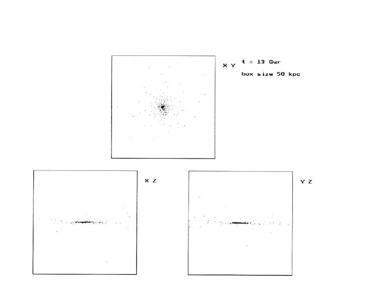
Fig. 4.: The distribution of ”gas” particles in the final step

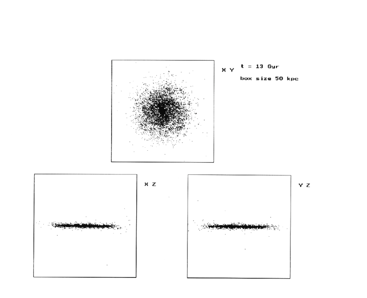
Fig. 5.: The distribution of ”star” particles in the final step

Fig. 6.: $\sigma_{gas}(r)$,$\sigma_{*}(r)$ and $\sigma_{tot}(r)=\sigma_{gas}(r)+\sigma_{*}(r)$. The column density distribution in the disk of gas and stars in the final step

Fig. 7.: $V_{rot}(r)$. The rotational velocity distribution of gas in the final step

Fig. 8.: $V_{rad}(r)$. The radial velocity distribution of gas in the final step

Fig. 9.: $V_{z}(r)$. The perpendicular to disk normal velocity distribution of gas in the final step

Fig. 10.: $T(r)$. The temperature distribution of gas in the final step

3.3 Chemical characteristics

Fig.11. shows the time evolution of the SFR in galaxy $SFR(t)=dM_{*}(t)/dt$. Approximately $90\%$ of gas is converted into stars at the end of calculation. The most intensive SF burst happened in the first $\approx 1$ Gyr, with a maximal SFR $\approx 35\;M_{\odot}/yr$. After $\approx 1.5-2$ Gyr the SFR is decreases like an ”exponential function” until it has a value $\approx 1\;M_{\odot}/yr$ at the end of the simulation. To check the SF and chemical enrichment algorithm in our SPH code, we use the chemical characteristics of the disk in the ”solar” cylinder ($8$ kpc $<\;r\;<\;10$ kpc).

The age–metallicity relation of the ”star” particles in the ”solar” cylinder, [Fe/H]$(t)$, is shown in Fig.12., with observational data taken from Meusinger et al.(1991) and Edvardsson et al.(1993), while in Fig.13. we presented the metallicity distribution of the ”star” particles in the ”solar” cylinder $N_{*}($[Fe/H]$)$. The model data are scaled to the observed number of stars ([Edvardsson et al. 1993]). In Fig.12. each model point represents the separate ”star” particle. The mass of each ”star” particle is different (from $\sim 10^{4}\;M_{\odot}$ up to $\sim 2.5\;10^{6}\;M_{\odot}$), because the star formation efficiency - $\epsilon$ is different in each star forming region. The model point is systematically higher than the observations (especially near the $t\approx 5$ Gyr), but if we also analyze the mass of each ”star” particle we see that the more massive particles systematically show lower metallicity than the observations. If one divides the metallicity to equal zone and calculate the sum of the mass in each metallicity zone in Fig.12. we get the results in Fig.13. and in this figure we see what the model mass distribution has shifted to the lower metallicities.

The [O/Fe] vs. [Fe/H] distribution of the ”star” particles in the ”solar” cylinder one found in Fig.14. In this figure we also present the observational data from Edvardsson et al.(1993) and Tomkin et al.(1992). All these model distributions are in good agreement, not only with presented observational data, but also with other data collected from Portinari et al.(1997).

The [O/H] radial distribution [O/H]$(r)$ is shown in Fig.15. The approximation presented in the figure is obtained by a least - squares linear fit. At distances $5$ kpc $<\;r\;<\;11$ kpc the models radial abundance gradient is $-0.06$ dex/kpc. In the literature we found different values of this gradient defined in objects of different types. From observations of HII regions ([Peimbert 1979]; [Shaver et al. 1983]) we obtained oxygen radial gradient $-0.07$ dex/kpc. From observations of PN of different types ([Maciel & Koppen 1994]) we obtained the values: $-0.03$ dex/kpc for PNI, $-0.069$ dex/kpc for PNII, $-0.058$ dex/kpc for PNIII, $-0.062$ dex/kpc for PNIIa, and $-0.057$ dex/kpc for PNIIb. All this agrees well with the oxygen radial gradient in our Galaxy.

Fig. 11.: $SFR(t)=dM_{*}(t)/dt$. The time evolution of the SFR in galaxy

Fig. 12.: [Fe/H]$(t)$. The age metallicity relation of the ”star” particles in the ”solar” cylinder ($8$ kpc $<\;r\;<\;10$ kpc)

Fig. 13.: $N_{*}($[Fe/H]$)$. The metallicity distribution of the ”star” particles in the ”solar” cylinder ($8$ kpc $<\;r\;<\;10$ kpc)

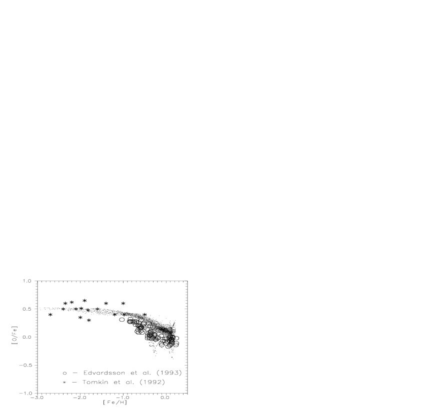
Fig. 14.: The [O/Fe] vs. [Fe/H] distribution of the ”star” particles in the ”solar” cylinder ($8$ kpc $<\;r\;<\;10$ kpc)

Fig. 15.: [O/H]$(r)$. The [O/H] radial distribution

3.4 Conclusion

This simple model provides a reasonable, self–consistent picture of the processes of galaxy formation and star formation in the galaxy. The dynamical and chemical evolution of the modeled disk–like galaxy is coincident with observations for our own Galaxy. The results of our modeling give a good base for a wide use of the proposed SF and chemical enrichment algorithm in other SPH simulations.

Acknowledgments. The author is grateful to S.G. Kravchuk, L.S. Pilyugin and Yu.I. Izotov for fruitful discussions during the preparation of this work. It is a pleasure to thank Pavel Kroupa and Christian Boily for comments on an earlier version of this paper. The author also thanks the anonymous referee for a helpful referee’s report which resulted in a significantly improved version of this paper. This research was supported by a grant from the American Astronomical Society.

References

- Alongi et al. 1993 Alongi M., Bertelli G., Bressan A., et al., 1993, Astron. & Astrophys. Suppl., 97, 851
- Bardeen et al. 1986 Bardeen J.M., Bond J.R., Kaiser N. & Szalay A.S., 1986, Astrophys. J., 304, 15
- Bennett et al. 1993 Bennett C.L., Boggess N.W., Hauser M.G., Mather J.C., Smoot G.F. & Wright E.L., 1993, in ”The Environment and Evolution of Galaxies”, Eds. Shull M.J., Thronson H.A.Jr., Kluwer Acad. Publ., 27
- Berczik & Kolesnik 1993 Berczik P. & Kolesnik I.G., 1993, Kinematika i Fizika Nebesnykh Tel, 9, No. 2, 3
- Berczik & Kravchuk 1996 Berczik P. & Kravchuk S.G., 1996, Astrophys. & Sp. Sci., 245, 27
- Berczik 1998 Berczik P., 1998, Presented as a poster in the Isaac Newton Institute Workshop: ”Astrophysical Discs”, June 22 - 27, 1998, Cambridge, UK. (astro-ph/9807059)
- Bertelli et al. 1994 Bertelli G., Bressan A., Chiosi C., Fagotto F. & Nasi E., 1994, Astron. & Astrophys. Suppl., 106, 275
- Bienayme 1998 Bienayme O., 1998, Astron. & Astrophys., 341, 86
- Burkert 1995 Burkert A., 1995, Astrophys. J., 447, L25
- Bressan et al. 1993 Bressan A., Fagotto F., Bertelli G. & Chiosi C., 1993, Astron. & Astrophys. Suppl., 100, 647
- Carraro et al. 1997 Carraro G., Lia C. & Chiosi C., 1997, Mon. Not. Roy. Astr. Soc., 297, 1021
- Dalgarno & McCray 1972 Dalgarno A. & McCray R.A., 1972, Annu. Rev. Astron. & Astrophys., 10, 375
- Dar 1995 Dar A., 1995, Astrophys. J., 449, 550
- Douphole & Colin 1995 Douphole B. & Colin J., 1995, Astron. & Astrophys., 300, 117
- Duerr et al. 1982 Duerr R., Imhoff C.L. & Lada C.J., 1982, Astrophys. J., 261, 135
- Edvardsson et al. 1993 Edvardsson B., Andersen J., Gustaffson B., et al.1993, Astron. & Astrophys., 275, 101
- Eisenstein & Loeb 1995 Eisenstein D.J. & Loeb A., 1995, Astrophys. J., 439, 520
- Ferriere 1995 Ferriere K.M., 1995, Astrophys. J., 441, 281
- Frenk et al. 1988 Frenk C.S., White S.D.M., Davis M. & Efstathiou G., 1988, Astrophys. J., 327, 507
- Friedli & Benz 1995 Friedli D. & Benz W., 1995, Astron. & Astrophys., 301, 649
- Greggio & Renzini 1983 Greggio L. & Renzini A., 1983, Astron. & Astrophys., 118, 217
- Hernquist & Katz 1989 Hernquist L. & Katz N., 1989, Astrophys. J. Suppl. Ser., 70, 419
- Hiotelis et al. 1991 Hiotelis N., Voglis N. & Contopoulos G., 1991, Astron. & Astrophys., 242, 69
- Hiotelis & Voglis 1991 Hiotelis N. & Voglis N., 1991, Astron. & Astrophys., 243, 333
- Katz & Gunn 1991 Katz N. & Gunn J.E., 1991, Astrophys. J., 377, 365
- Katz 1992 Katz N., 1992, Astrophys. J., 391, 502
- Kravtsov et al. 1997 Kravtsov A.V., Klypin A.A, Bullock J.S. & Primack J.R., 1997, Astrophys. J., 502, 48
- Kroupa et al. 1993 Kroupa P., Tout C. & Gilmore G., 1993, Mon. Not. Roy. Astr. Soc., 262, 545
- Larson 1969 Larson R.B., 1969, Mon. Not. Roy. Astr. Soc., 145, 405
- Leitherer et al. 1992 Leitherer C., Robert C. & Drissen L., 1992, Astrophys. J., 401, 596
- Lucy 1977 Lucy L.B., 1977, Astron. J., 82, 1013
- Maciel & Koppen 1994 Maciel W.J. & Koppen J., 1994, Astron. & Astrophys., 282, 436
- Matteucci & Greggio 1986 Matteucci F. & Greggio L., 1986, Astron. & Astrophys., 154, 279
- Mera et al. 1998a Mera D., Chabrier G. & Schaeffer R., 1998a, Astron. & Astrophys., 330, 937
- Mera et al. 1998b Mera D., Chabrier G. & Schaeffer R., 1998b, Astron. & Astrophys., 330, 953
- Meusinger et al. 1991 Meusinger H., Reimann H.G. & Stecklum B., 1991, Astron. & Astrophys., 245, 57
- Mihos & Hernquist 1996 Mihos J.C. & Hernquist L., 1996, Astrophys. J., 464, 641
- Monaghan & Lattanzio 1985 Monaghan J.J. & Lattanzio J.C., 1985, Astron. & Astrophys., 149, 135
- Monaghan 1992 Monaghan J.J., 1992, Annu. Rev. Astron. & Astrophys., 30, 543
- Moore et al. 1997 Moore B., Governato F., Quinn T., Stadel J. & Lake G., 1997, Astrophys. J., 499, L5
- Nomoto et al. 1984 Nomoto K., Thielemann F.-K. & Yokoi K., 1984, Astrophys. J., 286, 644
- Navarro et al. 1996 Navarro J.F., Frenk C.S. & White S.D.M., 1996, Astrophys. J., 462, 563
- Navarro et al. 1997 Navarro J.F., Frenk C.S. & White S.D.M., 1997, Astrophys. J., 490, 493
- Navarro 1998 Navarro J.F., 1998, Astrophys. J., submitted, (astro-ph/9801073)
- Navarro & White 1993 Navarro J.F. & White S.D.M., 1993, Mon. Not. Roy. Astr. Soc., 265, 271
- Peebles 1969 Peebles P.J.E., 1969, Astron. & Astrophys., 155, 393
- Peebles 1993 Peebles P.J.E., 1993, in ”Principles of Physical Cosmology”, Princeton Univ. Press
- Peimbert 1979 Peimbert M., 1979, in ”The Large Scale Characteristic of the Galaxy”, Ed. Burton W.B., Reidel, Dordrecht, p. 307
- Portinari et al. 1997 Portinari L., Chiosi C. & Bressan A., 1997, Astron. & Astrophys., 334, 505
- Raiteri et al. 1996 Raiteri C.M., Villata M. & Navarro J.F., 1996, Astron. & Astrophys., 315, 105
- Renzini & Voli 1981 Renzini A. & Voli M., 1981, Astron. & Astrophys., 94, 175
- Samland et al. 1997 Samland M., Hensler G. & Theis Ch., 1997, Astrophys. J., 476, 544
- Samland 1997 Samland M., 1997, Astrophys. J., 496, 155
- Shaver et al. 1983 Shaver P.A., McGee R.X., Newton L.M., Danks A.C. & Pottasch S.R., 1983, Mon. Not. Roy. Astr. Soc., 204, 53
- Silk 1987 Silk J., 1987, in IAU Symp. No. 115 ”Star Forming Regions”, Eds. Peimbert M., Jugaku J., Reidel, Dordrecht, p. 557
- Steinmetz & Muller 1994 Steinmetz M. & Muller E., 1994, Astron. & Astrophys., 281, L97
- Steinmetz & Muller 1995 Steinmetz M. & Muller E., 1995, Mon. Not. Roy. Astr. Soc., 276, 549
- Steinmetz & Bartelmann 1995 Steinmetz M. & Bartelmann M., 1995, Mon. Not. Roy. Astr. Soc., 272, 570
- Thielemann et al. 1986 Thielemann F.-K., Nomoto K. & Yokoi K., 1986, Astron. & Astrophys., 158, 17
- Tomkin et al. 1992 Tomkin J., Lemke M., Lambert D.L. & Sneden C., 1992, Astron. J., 104, 1568
- Vallee 1994 Vallee J., 1994, Astrophys. J., 437, 179
- van den Bergh & McClure 1994 van den Bergh S. & McClure R.D., 1994, Astrophys. J., 425, 205
- van den Hoek & Groenewegen 1997 van den Hoek L.B. & Groenewegen M.A.T., 1997, Astron. & Astrophys. Suppl., 123, 305
- Voglis & Hiotelis 1989 Voglis N. & Hiotelis N., 1989, Astron. & Astrophys., 218, 1
- Warren et al. 1992 Warren M.S., Quinn P.J., Salmon J.K. & Zurek W.H., 1992, Astrophys. J., 399, 405
- Wilking & Lada 1983 Wilking B.A. & Lada C.J., 1983, Astrophys. J., 274, 698
- White & Rees 1978 White S.D.M. & Rees M.J., 1978, Mon. Not. Roy. Astr. Soc., 183, 341
- White & Silk 1979 White S.D.M. & Silk J., 1979, Astrophys. J., 231, 1
- Woosley & Weaver 1995 Woosley S.E. & Weaver T.A., 1995, Astrophys. J. Suppl. Ser., 101, 181
- Zurek et al. 1988 Zurek W.H., Quinn P.J. & Salmon J.K., 1988, Astrophys. J., 330, 519