The correct analysis and explanation of the Pioneer-Galileo anomalies

Abstract

Tidal distension of spacecraft electronics due to spin and solar and galactic gravitation elegantly explains all variations in the anomaly reported by Anderson et al. Contrary to their conclusion, a constant residue seems to be present in lunar, terrestrial, and possibly planetary measurements, posing a problem of wider, more fundamental significance.

• 95.55.Pe, 95.30.Sf, 96.35.Fs, 95.10.Km

• Pioneer-10/11 anomaly, planetary ranging

I Introduction and overview

The Pioneer and other deep space missions employing spin-stabilised spacecraft have revealed an anomaly with characteristics that have defied a simple explanation [4]. What has been measured is a residual Doppler shift $\delta z$ in the telemetry signal, which has been generally interpreted as an acceleration by the gravitational redshift analogy

$$\delta g\sim r^{-1}\,c^{2}\,\delta z,$$ (1)

$r$ being the distance from the sun. Numerous mechanisms have been examined that could yield this force, including helium leakage and the reaction from power dissipation and radiation [5] [6], but to no avail [7] [8]. It has been noted that the anomaly is of the same order as the Hubble constant [9], or the cosmological time dilation (CTD) [10], but the standard model prohibits either on the planetary scale of distances: the hypothesis of expansion on smaller scales as such presents a logical difficulty [11, p.619] and matter appears to be gravitationally bound all the way up to the galactic scale. A modified theory of gravitation has also been considered hypothesising a changeover from $r^{-2}$ to $r^{-1}$ character that could produce this anomalous force, but it fails to explain the absence of the anomaly in the planetary ranging data [4]. The Pioneers also display an almost constant residual anomaly beyond $40$ AU, but with a persistent difference that again defies the equivalence principle [4], questioning the adequacy of any relativistic model whatsoever. Furthermore, even the residual value exhibits oscillations that display synchronicity with the earth’s orbital period, though measurement and analysis errors are stated to be ironed out.

These experiences indicate that the previous attempts have been simplistic in seeking a single cause for the anomaly and in viewing it as an actual acceleration, given the lack of visual or quadrature evidence to verify the inference. The frequency shift is not sufficient to imply a Doppler or gravitational cause, as any means to cause the onboard tuning devices and circuits to drop, or appear to drop, in frequency would lead to the same observation. Thermal and structural stresses can be presumably ruled out, since they would have been already considered in the design and the testing phases of the missions, but not mechanisms that would be ordinarily absent or too small to be routinely dealt with on earth. Such a mechanism cannot explain the constant remaining anomaly of either Pioneer, so a relativistic cause is still needed, but the latter cannot be sufficient by itself because of the violation of the equivalence principle, as mentioned.

Accordingly, we must consider a combination of such causes, thereby partitioning the anomaly into a constant part of the order of the Hubble constant, for which a relativistic explanation may yet be possible, and a variable part, whose path-dependence and oscillations, together with the fact that the anomaly has been observed only in spinning spacecraft, suggest a connection to the gravitational tidal forces due to the spin. This variable component is therefore attributed to an actual, physical expansion of the onboard electronics, in proportion to the tidal forces, making the transponder response frequency decrease without causing dynamical acceleration. Its analysis exclusively concerns the equivalent time dilation of the onboard clocks [4], which not only avoids the detracting notion of acceleration, but is factually closer to the actually measured quantity $\delta z$. It is convenient for this purpose, therefore, to define a “Hubble measure” for the acceleration,

$$h=c^{-1}\,\delta g,$$ (2)

having the same dimensions [$T^{-1}$] as the Hubble constant $H$, which describes the anomaly as if it were CTD, as explained in §III. We thus have the decomposition

$$h=h_{s}(r,\mathbf{\hat{\omega}})+h_{c}.$$ (3)

$h_{s}$ denoting the variable part due to tidal action, $\mathbf{\omega}$, the spin, and $h_{c}$, the constant part.

The possibility of tidal action stems from the smallness of the anomaly, $\sim 2.8\times 10^{-18}$ s^-1 [4], taking about $30$ y to stretch the spacecraft by $1$ nm, which explains why the electronic circuits have continued to function, albeit at gradually diminishing frequencies. It also explains, as we shall see, the proportionality of $\delta z$ to the expected tidal forces, which requires a notion of linearity; a larger rate of expansion would have caused non-linear variations in the behaviour of the circuits, disrupting their operation. We ordinarily expect the molecular bonding forces to prevent such a process, but we do have the example of glasses that “flow” slowly even under constant gravitational stress, and the repetitive shear stress due to the spin should cause a more rapid buildup of the microscopic fractures. Rheological degradation is allowed for in most component tolerances, but is too small to be modelled in engineering studies and very unlikely to have been considered in the spacecraft simulations. The tidal buildup also explains the manifestation of the anomaly in deep space, where gravity is much weaker than on the earth’s surface, and seems to correctly fit the oscillatory pattern in the Pioneer 10 anomaly. In any case, the possibility can be readily verified by spinning a test spacecraft on earth in powered-on state and continuously “ranging” it using telemetry.

Assuming these ideas to be correct, we would expect $h_{s}$ would be maximum when the spin $\mathbf{\omega}$ is perpendicular to the total gravitational force $\mathbf{g}$, and should vanish while inline, yielding three degrees of freedom in the model:

$$h_{s}=k_{s}(\phi)\,\omega^{\alpha}g^{\beta}\;|\mathbf{\hat{\omega}\wedge\hat{g}}|,$$ (4)

where $\phi$ denotes the angle of rotation and $k_{s}$, $\alpha$ and $\beta$ may vary between spacecraft (Fig. 1). The $\phi$-variation is expected because of the mechanical anistropy due to the rectangular layout of components on electronic circuit boards (Fig. 2), and is a prediction of the model. The earth-synchronism of Pioneer 10 oscillations is explained by the fact that the spin axis $\mathbf{\hat{\omega}}$ is generally made to follow the earth for the telemetry to be possible at all (Fig. 3). The persistent remaining difference in the Pioneer anomalies seems to fit the asymmetric vector contribution expected from the galactic gravitational field (Fig. 4). A determination of $k_{s}(\phi)$, $\alpha$ and $\beta$ in the laboratory would therefore provide a useful tool for analysing the galactic gravitational field. The detailed application of $h_{s}$ to the reported characteristics of the anomaly is given in §II.

The absence of the anomaly in planetary data is partly explained by the lack of a transponder to reproduce $h_{s}$ and its variations. The constant portion $h_{c}$ presents some difficulty, as it implies a uniform slowing of clocks, like the CTD, in the planetary space, questioning the standard model assumptions, as already mentioned. Its similarity to the CTD implies, however, that $h_{c}$ could manifest as a Hubble flow, i.e. in proportion to the range, rendering Anderson et al’s consideration of the inner planet ranging data insufficient for claiming the absence of the anomaly in planetary motion, especially given that all six missions specifically involve $r>1.3$ AU [4]. A search for Hubble flow-like evidence in planetary, lunar and terrestrial data does turn out to be positive (§III).

A complete explanation of the anomaly is thus claimed in the context of the deep space missions. It is further concluded that $h_{c}$ can and should be explained in a wider context, on grounds that we are otherwise able to account for all of the discernible details in the NASA-JPL reports, as explained in the next section, and that the deep space ranging appears to be the first means capable of verifying the absence of planetary CTD or Hubble flow in the first place, and may be indicative of new physics.

II Application of the model

Accordingly, the following principal characteristics of the anomaly are sought to be explained by the model:

1. Differs from planetary ranging [4] and between the spacecraft and missions [7]:

   1. Does not manifest in planetary ranging.

   2. Earth clock drift fits Doppler but not range.

   3. Fitting a line-of-sight acceleration leads to sign inconsistency.

   4. Speed of light correction to the planetary forces does not fit Galileo.

   (A1) has been partly explained by the fact that the ranging procedure is indeed different from that of planetary ranging, as it employs a generated return and not an actual reflection. Completeness of (A1) is questioned since only inner planet range data has been used in arriving at the conclusion, whereas the spacecraft displaying the anomaly are invariably at $r>1.3$ AU and generally about or beyond the outer planet distances.

   (A2-A4) are the reasons for the present view that the variable part $h_{s}$ cannot mean actual acceleration and must be explained as a slowing down of the spacecraft clocks, which can depend on the composition and motion parameters of the individual spacecraft.

2. Fluctuations and periodicities [7]:

   1. Sinusoidal variation with earth-year periodicity (Pioneer 10: 1987-1994).

   2. Maxima larger than minima, data points wilder near the minima (Pioneer 10).

   3. More fluctuations later (Pioneer 10: mid-year after 1993, more frequent after 1996).

   These cannot be explained by modified gravitational field theories [4], and force-generating mechanisms like leakage and radiation have already been ruled out as unlikely, along with systematic observation error that might be inferred from (B1) [7]. These features are well explained in the present model by the targeting of the spin axis $\mathbf{\hat{\omega}}$ towards the earth.

3. Range dependence:

   1. Higher in nearer orbits (Ulysses vs. Pioneers), not matching $r^{-2}$ [4].

   2. Linear weakening from Jupiter to somewhere $>40$ AU (Pioneer 10: 1987-1994) [7].

   3. Eventually levels off (both Pioneers) [4] [7].

   4. Continues to differ between the two Pioneers as they head out of the solar system [4] [7].

   5. Remains larger than $H$, at $\sim 84$ km/s-Mpc.

   (C5) parallels other data that seem to confirm the general occurrence of $h_{c}\approx H$ on the planetary scale, to be discussed in §III.

Fig. 1 illustrates the basic quantities in the model (eq. 4). Each spacecraft is approximately cylindrical, and carries the main antenna on one end, which is generally kept pointing towards the earth by spin stabilisation and correcting manoeuvres. For this, the spin axis must point towards the earth, so that it subtends the angle $\theta$ to the net gravitational force $\mathbf{g}$, presumably due to the sun. As the spacecraft moves, the value of $\theta$ changes, causing $h_{s}$ to vary even if $\omega$ were constant, as likely in the closed orbit missions, and differently from the $r^{-2}$ nature of $\mathbf{g}$. Additionally, the construction must invariably result in a mechanical anisotropy, illustrated in Fig. 2, which should cause $h_{s}$ to vary with the spin rotation angle $\phi$, tracing out a hysterisis loop along each of the tranverse principal axes. The Pioneer 10 plots given by Turyshev et al show only $50$ day averages [7], but continuous telemetry may have occurred during Galileo’s earth fly-by, and might reveal high frequency oscillations due to this anisotropy.

Fig. 3 illustrates the orbital variation of $\theta$ that explains (B1)-(B3), (C1), (C2) and (C4). $S$ denotes the sun and $A$, $B$, $C$ and $D$, successive positions of the earth along its orbit. If the spacecraft stays in the plane of the ecliptic, as indicated by point $P_{0}$, its spin axis would be pointing directly towards the sun when the earth is at $A$ or $C$, so that $\theta=0$ and there would be no $h_{s}$ contribution at these times. $|\theta|$ reaches its maximum $\theta_{0}=\angle BP_{0}S=\angle DP_{0}S$, when the earth is at $B$ or $D$, so that $h_{s}$ should peak twice a year. In the case of non-ecliptic spacecraft, as indicated by point $P_{1}$, $\theta$ would again have two maxima, $\theta_{1}$ and $\theta_{2}$, but they would be now unequal and occur at different times, $A$ and $C$. At points inbetween $P_{0}$ and $P_{1}$, however, the spacecraft would be seasonally occluded by the sun when the earth is near $A$, in which case, earth-targeting manoeuvres and measurements are both impossible. This difference between ecliptic and non-ecliptic paths may be responsible for the sign difference in (A3).

The model clearly has adequate degrees of freedom to explain the details of the anomaly. For instance, it is about $400\times 10^{-18}$ s^-1 ($12\times 10^{-8}$ cm/s^-2) for Ulysses, which orbits the sun at $1.3<r<5.2$ AU, and is larger than in the case of the Pioneers. (C1). As $\theta$ is small at $r\gg 1$ AU, it can contribute a linear ($r^{-1}$) variation. For example, between $5$ AU (Jupiter) and $40$ AU (Neptune and Pluto), $\max(\theta)$ drops from $11.32\hbox{${}^{\circ}$}$ to $1.43\hbox{${}^{\circ}$}$, yielding a factor of $7.8\approx 40/5$ in $\sin(\theta)$ and thence in $h_{s}$, all other factors remaining the same. In the case of Pioneer 10, the spin rate $\omega$ was also decreasing upto mid-1990 (C2), and $\alpha$ is very likely to be $1$, the $\theta$ variation cannot be the sole cause of this decrease. In any case, $\beta$ is likely to be fractional, and the smallness of $|k_{s}|$ relative to $h_{c}$ may be sufficient to mask out non-linear details. Additionally, since $|\sin(\theta)|$ is at most $1$, the anomaly is rendered incapable of rising much further at perihelions closer than $1$ AU to the sun.

(C3) and (C4) are elegantly explained by considering the vector sum of the solar and the galactic gravitational forces $\mathbf{g}=\mathbf{g}_{s}+\mathbf{g}_{g}$ acting on the spacecraft (Fig. 4). As the spacecraft are headed in opposite directions from the sun, their spins must be approximately in line with the sun, at least so long as their signals were being received. Had their headings been also perpendicular to the galactic centre, $\mathbf{g}$ would have been symmetrical with respect to the sun, and the expansion rates would have been equal in that case. Pioneer 10 is, however, headed in the direction of the galactic centre, so the vector sum $\mathbf{g}$ is neither equal nor symmetric about the spin axis. The galactic component $\mathbf{g_{g}}$ is shown greatly exaggerated: in the limit of small $\mathbf{g_{g}}$, where $\theta\approx\pi/4$, the magnitude of the sum, $|\mathbf{g}|$, varies more rapidly than $\sin(\theta)$, explaining the larger anomaly of Pioneer 11. This not only explains the disparity, but confirms that the spacecraft are indeed still expanding, since $h_{c}$ may not be due to expansion.

As remarked by Turyshev et al, the spin deceleration of $4.73\times 10^{-6}$ s^-2 ($0.065$ rev/day/day) would have contributed to the linear decrease seen in the Pioneer 10 graphs [7], but we do not have the data to determine $\omega$ at any point, in order to determine the exact contribution, from which $\beta$ could have been determined, assuming $k_{s}(\phi)\approx\alpha=1$. The absence of a semi-annual maximum upto mid-1996 (B1) is generally explained by occlusion by the sun (point $A$ in Fig. 3), given that Pioneer 10 has not been too far from the ecliptic. Being cumulative, (eq. 1 in [7]), the anomaly would continue to grow at the rate set by the last targeting manoeuvre during the occlusion. We do not know how frequently the targeting manoeuvres were being performed, but it seems less likely that they would have been needed from near $A$, where $\theta$ changes the least, than from points $E$ and $F$, before and after the occlusion, respectively, and is most likely around $C$, where $\theta$ varies most rapidly. This would explain why the maxima are larger, and the lower data points are more scattered (B2) because the spin is allowed to drift on the side of $A$. There are a few data points very close to the best-fit minima (mid-1987, mid-1988), which at first sight seem to contradict the occlusion idea, but these too can be attributed to the cumulative nature of the anomaly.

Changes in the spin rate have clearly contributed to the variations between mid-1990 and mid-1992. The gradual appearance of more humps thereafter is probably due to drift of the spin axis, as a re-targeting was needed in Jan 1997. The spin has been otherwise steady, explaining the levelling out of the anomaly (C3).

III Constant part of the anomaly

As already remarked, the ranging data from the two nearest planets Venus and Mars [4] is not sufficient for concluding that the (constant part $h_{c}$ of the) anomaly is absent in the planetary data, because

1. the measured anomalous quantity is the frequency shift $\delta z$, not an actual acceleration unambiguously determined by visual or quadrature means;

2. interpretation as actual acceleration does not fit the data (A2-A4), regardless of whether it is ascribed to leaking and dissipation or to modified gravity; and

3. the anomaly has been observed exclusively in deep space beyond Mars, not in near space missions.

Items (a) and (b) particularly imply that the true nature of the anomaly lies only in the spacecraft time dilation, or an equivalent expansion of onboard clocks, which is how the tidal expansion $h_{s}$ was deduced. The expansion of clocks does not imply a uniform expansion of space, as $h_{s}$ itself illustrates, but a uniform expansion, if present, would include the expansion of clocks, yielding a redshift. The associated Hubble’s law recession

$$\dot{r}_{c}=h_{c}\,r$$ (5)

implies an increasing optical path $r\sim ct$, hence, if we did not know the cause, we would only observe the apparent acceleration

$$\ddot{r}=\frac{d}{dt}\{h_{c}\,ct\}=h_{c}\,c,$$ (6)

equivalent to eq. (2), in this case. This is substantially the derivation used by Rosales and Sanchez-Gomez [9].

Anderson et al looked for a radial acceleration, which would have measurably perturbed the orbital radius and period [4], but this is insufficient in the context, as the anomaly could have been caused, according to eq. (6), by an unmodelled recession instead of static perturbations. The absence of recession cannot be verified by a one-time observation because of the smallness of $h_{c}\approx H$ (C5): the expectable recession velocities would be only $1.6$ $\mu$m/s for Jupiter $5$ AU) and $12.5$ $\mu$m/s for Neptune/Pluto ($40$ AU), too small to be detected by Doppler measurement. The only way to detect the ongoing recession, if any, is to look for cumulative displacements over a long enough period, say a year, as listed in Table I below. The fact that the standard model does not support this possibility is not relevant to this test, in part because this notion of the standard model has itself never been empirically verified, $H$ being too small to have inadvertently shown up on any scale short of the galactic.

The table further shows why it is incorrect to compare with Venus or Mars - even their annual recessions with respect to earth would be only about $2$-$6$ m, less than a twentieth of the precision, $100$-$150$ m, available for the earth and Mars orbital radii from the Viking data [4]. One would ordinarily expect that by now, the measurements would have been repeated, with a gap of at least three years, so that the recession, if present, would have been noticed already. Our research reveals that such differences have been reported at least twice, once for Mercury, but were treated both times as systematic error. The recent instance is finding Jupiter $11$ km farther, in 1992, than predicted, presumably from data acquired in the 1970s [18], indicating a recession of $611$ m/y, or $H\approx 770$ km/s-Mpc, about $10$ times the possible Hubble flow. Incidentally, due to its angular limit of resolution, the ranging precision follows a “Hubble’s law” of its own

$$\delta r\sim h_{\mu}\,r,$$ (7)

where $h_{\mu}$ is characteristic of the measuring technique. As a result, the presence or absence of Hubble flow can be decided only by improving the sensitivity by at least two orders of magnitude. Since this is precisely the capability in effect achieved by the spacecraft ranging technique used in the deep space missions, the indication of $h_{c}$ may verily mean the presence of a planetary Hubble flow.

It is of paramount importance, therefore, to look for it at even smaller scales, using more precise means that are generally available because of proximity. The logical difficulty referred to earlier should prevent the flow from manifesting on the scale of the internal structure of matter, but since physics cannot rest on logic alone, this too needs to be empirically verified. We do find positive indications on lunar and geophysical scales, as follows.

The moon is known, from very precise measurements, to be receding at $3.84$ cm/y [12], which is large enough to accomodate the anomaly along with the known tidal cause for the recession, there being no independent means of measuring the tidal contribution. The tidal action is also responsible for the slowing down of earth’s rotation, and remarkably, this and other geological evidence have indicated that the earth may have been expanding in the past [13] [14] [15] [16]. The indictated values of $0.4$-$0.6$ mm/y correspond to the range $61$-$92$ km/s-Mpc for $H$ [17], of which a small part could still account for the tidal action, so that the anomaly cannot be easily ruled out even in this case.

IV Conclusion

We have essentially established that there could be two distinct causes underlying the anomaly, one of which ($h_{s}$) is associable with an actual stretching of the spacecraft and its electronics due to gravitational tidal action from its spin, and is dependent on the individual spacecraft and its motion. The presence of $h_{s}$ may be responsible for the contradictory results obtained when various models to explain the constant acceleration ($h_{c}$) are applied to the data. It has been further shown that $h_{s}$ fits the anomaly in greater detail than any of the uniform gravitational and other force models previously attempted.

It has been also shown that Anderson et al’s conclusion that $h_{c}$ is absent in planetary data, is premature, as a uniform expansion of space could cause the time dilation and give the appearance of acceleration, without showing up even cumulatively in planetary ranging data, let alone manifest in the Doppler residuals. The possibility appears to be no more offbeat or remote than the modifications to gravitation theory they have considered. More importantly, our analysis shows that the anomaly may itself be the first tool precise enough to measure the planetary flow and the galactic gravitation, and may yet be pointing to significant new physics.

An illustrative potential application is the resolution of Arp’s quasars and galaxies that exhibit redshifts in excess of the Hubble flow and in quantised increments [19]. Every such object appears to be (a) spinning and (b) in intimate proximity of a much larger galactic body, like the Galileo and Pioneer spacecraft in relation to the sun, suggesting that $h_{s}$ may be responsible for these anomalies as well.

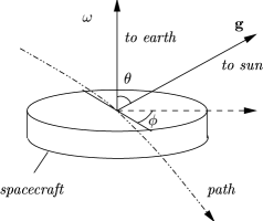
FIG. 1.: Geometry of the anomaly

FIG. 2.: Spacecraft construction schematic

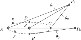
FIG. 3.: Orbital geometry

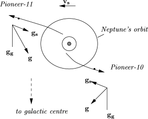
FIG. 4.: Galactic contribution geometry

Body	Distance			Recession (m/y)
	(AU)			$h_{c}=50^{\dagger}$	$h_{c}=75^{\dagger}$
Moon‡	$2.57\times$		$10^{-4}$	0.0197	0.0295
Mercury	0	.	40	30	44
Venus	0	.	72	55	83
Earth	1	.	00	77	115
Mars	1	.	52	117	175
Jupiter	5	.	20	398	597
Saturn	9	.	56	731	1,096
Uranus	19	.	19	1,468	2,202
Neptune	30	.	11	2,303	3,455
Pluto	39	.	53	3,024	4,535

TABLE I.: Planetary Hubble flow

REFERENCES

- [1]
- [2]
- [3]
- [4] J D Anderson et al, Indication from Pioneer 10/11, Galileo and Ulysses Data of an Apparent Anomalous, Weak, Long-Range Acceleration, Phys Rev Lett, Oct 1998.
- [5] E M Murphy, A Prosaic Explanation for the Anomalous Acceleration…, gr-qc/9810015, Oct 1998.
- [6] J I Katz, Comment on “Indication from Pioneer 10/11…” gr-qc/9809070, Dec 1998.
- [7] S G Turyshev et al, The Apparent Anomalous…, XXXIV Rencontres de Moriond, France, Jan 1999, gr-qc/9903024, Mar 1999.
- [8] J D Anderson et al, replies to [5], gr-qc/9906113, and to [6], gr-qc/9906112, Jun 1999.
- [9] J L Rosales and J L Sanchez-Gomez, A Possible Cosmological Origin of the Indicated Anomalous Acceleration…, gr-qc/9810085, Oct 1998.
- [10] R Ellman, An Interpretation of the Pioneer 10/11 …, Phys Rev Lett, Vol 81, No 14, 5 Oct 1998.
- [11] C W Misner, K S Thorne and J A Wheeler, Gravitation (W H Freeman and Co, 1973).
- [12] J O Dickey et al, Lunar Laser Ranging: A Continuing Legacy of the Apollo Program, Science, Vol 265, 22 July 1994.
- [13] P S Wesson, The implications for geophysics of modern cosmologies in which is variable, Quarterly J of Roy Astro Soc, 9-64, 1973.
- [14] K M Creer, An expanding earth?, Nature, 205, 539, 1965.
- [15] S K Runcorn, Earth, possible expansion of, p383-389, Intl Dict of Geophysics, Pergamon, 1967.
- [16] P S Wesson, private communication, 13 Sep 1999.
- [17] J MacDougall et al, A comparison of terrestrial and universal expansion, Nature, 199, 1080, 1963.
- [18] J K Harmon et al, Radar ranging to Ganymede…, Astro J, Vol 107, No 3, 1175-1181, March 1994.
- [19] H C Arp, Quasars, Redshifts and Controversies, Interstellar Media, Berkeley, CA 94705, 1988.