SN 1994D in NGC 4526: a normally bright type Ia supernova

Abstract

SN 1994D of type Ia has been suspected not to fit into the relation between decline rate, colour, and brightness. However, an individual distance of its host galaxy, NGC 4526, other than that of the Virgo cluster, has not yet been published. We determined the distance by the method of globular cluster luminosity functions on the basis of HST archive data. A maximum-likelihood fit returns apparent turn-over magnitudes of $23.16\pm 0.16$ mag in $V$ and $21.96\pm 0.09$ mag in $I$. The corresponding distance modulus is $30.4\pm 0.3$ mag, where the error reflects our estimation of the absolute distance scale. The absolute magnitudes (not corrected for decline rate and colour) are $-18.67\pm 0.30$ mag, $-18.62\pm 0.30$ mag, and $-18.40\pm 0.30$ mag for $B$, $V$, and $I$, respectively. The corrected magnitudes are $-18.69\pm 0.31$ mag, $-18.69\pm 0.31$ mag, and $-18.44\pm 0.31$ mag.

Compared with other supernovae with reliably determined distances, SN 1994D fits within the errors. It is therefore not a counter-example against a uniform decline-rate–colour–brightness relation.

1 Introduction

Supernovae (SNe) of type Ia are the best standard candles in the universe. Hamuy et al. (hamuy:96 (1996)) showed how remarkably small the brightness dispersion among SNe Ia is, for a sample of high observational quality. Moreover, decline rate and colour at maximum phase can be used to introduce corrections and to squeeze the dispersion even below $0.15$ mag in $B$, $V$, and $I$ (Tripp tripp:98 (1998); Richtler & Drenkhahn richtler:99a (1999)). But a few SNe have been observed which apparently do not fit with the Calán/Tololo sample of Hamuy et al.; the prominent cases being SN 1991bg in NGC 4347, SN 1991T in NGC 4527, and SN 1994D in NGC 4526, which are too bright/faint/red etc. However, checking the literature, one finds that the claim for anomaly often relies on indirect arguments, i.e. without a reliable knowledge of the distance of the host galaxy. For example, SN 1994D was labelled “anomalous” by Richmond et al. (richmond:95 (1995)), based on a comparison with SN 1989B in M66 and SN 1980N in NGC 1316, which made SN 1994D appear too bright by $0.5$ mag. A disadvantages is that M66 only has a Tully-Fisher distance, for which it is known that large residuals to the mean relation exist for individual galaxies. Moreover, this method suffers from uncertain extinction, which, together with the dispersion in the Tully-Fisher relation, results in an error in the absolute magnitude of the order $0.25$ mag (Jacoby et al. jacoby:92 (1992)). On the other hand, the distance modulus of NGC 1316 was adopted as $31.02$ mag while globular clusters (GCs), Cepheids, and surface brightness fluctuation (SBF) measurements (Kohle et al. kohle:96 (1996), Della Valle et al. dellavalle:98 (1998), Madore et al. madore:98 (1998), Jensen et al. jensen:98 (1998)) now agree on a value of $\sim 31.35$ mag for the Fornax Cluster distance modulus. Due to the cluster’s compactness we identify the distance to NGC 1316 with the cluster distance. An up-to-date discussion of the Fornax Cluster distance can be found in Richtler et al. (richtler:99b (1999)).

Sandage & Tammann (sandage:95 (1995)) also found SN 1994D too bright by 0.25 mag. They used the fact that NGC 4526 is a member of the Virgo cluster and based their comparison on other Virgo SNe. While the difference may be marginal, any correction for the decline rate would increase the discrepancy, hence rendering the decline-rate–luminosity relation not generally valid. However, no individual distance for NGC 4526 has yet been published. The distance value used by Richmond (richmond:95 (1995)) and Patat (patat:96 (1996)) is an unpublished SBF distance modulus of $30.68\pm 0.13$ mag from Tonry. In this paper, we shall give a distance for NGC 4526, derived by the method of globular cluster luminosity functions (GCLFs) (e.g. Whitmore whitmore:97 (1997)), and we want to demonstrate that the brightness of SN 1994D fits reasonably well to the Fornax SNe.

2 Data and reduction

2.1 Data

Our data consist of HST-WFPC2 images and have been taken from the HST archive of the European Coordinating facility at ESO. Table 1 lists the exposure times and filters associated with the data. The date of the observation was May 8th, 1994 (Rubin rubin:94 (1994)). Pipe-line calibration was done with the most recent calibration parameters according to Biretta et al. (biretta:96 (1996)). All frames were taken with the same pointing and the photometry was performed on averaged frames with an effective exposure time of 520 s each.

Hot pixels were removed with the IRAF task WARMPIX. The limited Charge Transfer Efficiency was corrected for with the prescriptions given by Whitmore & Heyer (whitmore_heyer:97 (1997)). Cosmics were identified with the IRAF task CRREJ and eventually the frames were combined with a weighted average.

We modelled the galaxy light with the IRAF task IMSURFIT and achieved a very satisfying subtraction of the galaxy light with no visible residuals. After this, the photometric effects of the image distortion were corrected for by a multiplication with a correcting image (Holtzman et al. holtzman:95 (1995)).

Table 1: The names of the respective HST data set, the filter, and the exposure time in seconds.

Name	Filter	$t_{\mathrm{exp}}$
u2dt0501t	F555W	60
u2dt0502t	F555W	230
u2dt0503t	F555W	230
u2dt0504t	F814W	60
u2dt0505t	F814W	230
u2dt0506t	F814W	230

2.2 Object search and photometry

Due to the Poisson noise of the galaxy light, one finds a noise gradient towards the centre of the galaxy. The normally used finding routine DAOFIND from the DAOPHOT package (Stetson stetson:87 (1987)) does not account for a position-dependent background noise. Using DAOFIND with a mean noise level results in many spurious detections near the galaxy centre and missed objects in regions with lower noise background. Therefore we used the finding routine of the SExtractor program (Bertin & Arnouts bertin:96 (1996)). The lower threshold was adjusted in order to include also the strongest noise peaks with a number of connected pixels of $3$ and a threshold of $1.4\cdot\sigma$. Our initial object list consists of 304 found and matched objects in the three wide-field frames of the F555W and F814W images. The planetary camera data were not used because they showed only very few globular cluster-like objects.

For these objects aperture photometry (with DAOPHOT) has been obtained through an aperture of $0\aas@@fstack{\prime\prime}5$. These instrumental magnitudes were finally corrected for total flux and transformed into standard Johnson magnitudes with the formulae given by Holtzman et al. (holtzman:95 (1995)).

3 The luminosity function

3.1 The selection of globular cluster candidates by elongation, size and colour

The selection of cluster candidates in HST images benefits greatly from the enhanced resolution. While in ground-based imaging, cluster candidates often cannot be distinguished from background galaxies, this problem is less severe in HST images. Galaxies that are so distant that their angular diameter is comparable to cluster candidates in NGC 4526, normally have quite red colours. Remaining candidates are foreground stars and faint background galaxies, where the redshift balances an intrinsic blue colour. Our strategy, described in more detail below, is the following: we first select our sample with respect to the elongation as given by the SExtractor program, then the angular size measured as the difference between two apertures, and finally the colour.

3.1.1 Elongation

The elongation is taken as the ratio $E=A/B$, where $A$ and $B$ are the major and the minor axes as given by SExtractor. However, the undersampling can cause a spurious elongation if a given object is centred between 2 pixels. We therefore chose $E<1.9$ in both filters to exclude only the definitely elongated objects.

3.1.2 Size

The SExtractor stellarity index is not very suitable for undersampled images because the neural network of SExtractor is trained with normally sampled objects (Bertin & Arnouts bertin:96 (1996)). We use the magnitude difference in two apertures as a size measure (Holtzman et al. holtzman:96 (1996)). These apertures should be compatible with the expected size of a GC in NGC 4526. A typical half-light radius of a GC is of the order of a few pc. Thus the larger clusters are marginally resolvable, assuming a distance of 13 Mpc to NGC 4526, which corresponds to 6 pc per pixel. The parameter $m_{12}:=m_{1}-m_{2}-(m_{1}-m_{2})_{*}$ is defined as the magnitude difference between one and two pixel apertures $m_{1}-m_{2}$ minus the appropriate value for a star-like object $(m_{1}-m_{2})_{*}$. The latter subtraction accounts for the position-dependent PSF of the WFPC2.

To find a reasonable size limit, we simulated cluster candidates by projecting the data for Galactic GCs at a distance of 13 Mpc, based on the McMaster catalogue of Galactic globular clusters (Harris harris:96 (1996)). We generated oversampled King-profiles (King king:62 (1962)) with the geometric parameters from this catalogue and convolved them with an oversampled PSF of the WFPC2. The resulting images were rebinned at four different subpixel positions giving WFPC2 images of the Galactic globular cluster system (GCS) as it would be observed from a distance of 13 Mpc. Fig. 1 shows the measured $m_{12}$ values as functions of the core radii $r_{c}$. It turns out that $m_{12}$ is a sufficiently good quantity to measure $r_{c}$.

Figure 1: The measured $m_{12}$ values of the simulated Galactic GCs as a function of the core radius $r_{c}$. Every GC is represented by 12 crosses according to the 3 WF cameras and 4 different subpixel positions.

Applying a selection criterion of $m_{12}<0.45$ in both filters excludes extended GCs with $r_{c}>5$ pc. This reduces the size of the GC sample but does not introduce a bias because $r_{c}$ and $M_{V}$ are not correlated. The $m_{12}$ magnitude is not suitable to place a lower size limit because the smaller GCs are unresolved and cannot be distinguished from a stellar-like image.

Fig. 2 compares the distribution of $m_{12}$ of the sample of our detected sources with that of the simulated clusters for both filters. The dotted histogram represents the background sources (see Sec. 3.3). The objects with $m_{12}>0.45$ can be almost entirely explained as resolved background objects.

Figure 2: These histograms show the distribution of $m_{12}$ for the detected sources (upper panel) and the simulated clusters (lower panel). The dotted histogram shows the expected background objects (=galaxies) derived from the Medium Deep Survey frames. Objects with values $m_{12}>0.45$ are resolved and mostly background objects. The distribution for F814W is essentially the same.

3.1.3 Colours

The range of existing colours among Galactic GCs is not a very good guide in our case: large error bars and a possibly different metallicity distribution may cause a different shape of the colour histogram. However, as Fig. 3 shows, a selection with regard to shape and size selects also according to colours, i.e. the redder objects, which are presumably redshifted background galaxies, can be effectively removed.

The colour histogram of the remaining objects shows some similarity to other GCSs with regard to the apparent “bimodality”, for example in M87 (Whitmore et al. whitmore:95 (1995)). One may suspect that there is a dichotomy in the population of GCs in the sense that the blue (=metal poor) objects belong to a halo population and the red ones to the bulge. Unfortunately, the number of objects found does not allow a deeper investigation. The mean colour is $\langle V-I\rangle=1.1$.

Figure 3: This colour histogram shows the shape- and size-selected sample of objects. The dotted line denotes the distribution of the complete sample. It can be seen that the shape and size distribution can already discriminate against red objects which are presumably distant galaxies. For the final sample, we chose the colour interval $0.8<V-I<1.4$.

We also exclude very faint objects with large photometric errors $\Delta m>0.3$ in at least one of the two filters. They hardly contribute to the determination of the turn-over magnitude (TOM) because of their large uncertainty.

3.2 Completeness

The completeness $I(m)\cdot\mathrm{d}m$ is the probability of finding an object in the magnitude interval $[m,m+\mathrm{d}m]$. On frames with a homogeneous background, it depends mainly on the brightness of an object. In our case, where the object search was done on a frame with a subtracted galaxy, the noise of the background $\rho$ varies strongly, and must be treated as a second parameter in $I(m;\rho)$.

We evaluated the completeness in our $V$, $I$ sample by inserting artificial objects in the $V$-frame and we used the same coordinates for inserting objects in the $I$-frame, after having fixed the colour for all objects to the value of $V-I=1.1$. In total we used 19000 artificial “stars” in the magnitude range $23<V<25.5$ and evaluated the completeness in bins of 0.1 mag. The noise as the second parameter is taken to be the standard deviation $\rho$ of pixel values in the annulus used by the aperture photometry. In practice, we used three completeness functions for three different $\rho$-values $1.75$ DN, $2.05$ DN, and $3.35$ DN, which represent the intervals $[1.6,1.9]$, $[1.9,2.2]$, and $[2.2,4.5]$, respectively.

Fig. 4 shows the completeness for the three noise intervals and for the two filters. The distinct difference between the three curves demonstrates that $\rho$ is indeed a reasonable parametrisation.

Figure 4: The completeness for $V$ and $I$ for three different noise intervals, which are characterised by the mean values $\rho=1.75$ DN, $2.05$ DN and $3.35$ DN (from right to left) in the $V$ filter.

3.3 Foreground and background sources

The field of our HST images is too small for a proper analysis of the contaminating background sources that survived all selection processes.

Therefore, we used the WFPC2 Medium Deep Survey (MDS) (Ratnatunga et al. ratnatunga:99 (1999)) to obtain an estimation of the background. Suitable fields should be possibly nearby, in particular regarding the Galactic latitude, and should be deep with several single exposures. We found the exposures which are listed in Table 2 together with some information. The frames are deep enough (in F606W and F814W) that the source finding is complete in the relevant magnitude interval. $V$ and $I$ magnitudes are calculated according to the prescriptions of Holtzman et al. (holtzman:95 (1995)).

Table 2: The exposures from the Medium Sky Survey which have been used for the background evaluation. Given are the data set names, total exposure times in seconds, and the number of individual frames, which entered the averaging process.

	$t_{\mathrm{exp}}$ [s]	$t_{\mathrm{exp}}$ [s]	#	#
Name	in F606W	in F814W	in F606W	in F814W
u30h3	1200	1266	6	8
uy400	866	1000	6	6
uy401	600	700	4	8
uyx10	800	700	3	3
uzx01	696	1550	5	4

The selection criteria discussed above are applied in exactly the same way as in the case of the NGC 4526 frames. It turns out that most background objects are selected out. The Poisson scatter of background objects from frame to frame is in the expected statistical range. Thus any clustering in the background galaxy number density does not influence the background LF. So we can assume that the background LF derived from the MDS frames gives also a good estimate for the background LF near NGC 4526.

As can be assessed also from Fig. 2, the fraction of background objects in the selected samples is only 7%. The resulting luminosity function $b(m)$ enters the maximum-likelihood fitting process as described in Sec. 3.4.1.

3.4 The turn-over magnitude

3.4.1 Remarks on the maximum-likelihood fit and the TOM of NGC 4526

For the representation of the GCLF, we choose the $t_{5}$-function, which has been shown to be the best analytical representation of the Galactic GCLF and that of M31 (Secker secker:92 (1992)). It reads

$$t_{5}(m;m^{0},\sigma_{t})=\frac{8}{3\sqrt{5}\pi\sigma_{t}}\left(1+\frac{(m-m^{0})^{2}}{5\sigma_{t}^{2}}\right)^{-3}.$$ (1)

The maximum-likelihood fitting method evaluates the most probable parameters for a given distribution $\phi$ by maximising the likelihood

$$L(m^{0},\sigma_{t})=\prod_{i}\phi(m_{i};m^{0},\sigma_{t}).$$ (2)

For the theoretical background of this method see Bevington & Robinson (bevington:92 (1992)), Caso et al. (caso:98 (1998)). Secker (secker:92 (1992)) and Secker & Harris (secker:93 (1993)) already applied it to the fitting of GCLFs.

What is to be fitted is the $t_{5}$-function modified by the different influencing factors, i.e. the completeness, the background, and the photometric errors. We used an extended version of the distribution of Secker (secker:92 (1992)) that accounts for a position-dependent background noise.

$$\begin{array}[]{l}\phi(m;\rho,m^{0},\sigma_{t})=\\ \quad K\cdot\kappa(m;\rho,m^{0},\sigma_{t})+(1-K)\cdot\beta(m;\rho)\end{array}$$ (3)

with $\kappa$ being the normalised distribution of the GCs

$$\begin{array}[]{l}\kappa(m;\rho,m^{0},\sigma_{t})=\\ \quad I(m;\rho)\cdot\left(\int t_{5}(m^{\prime};m^{0},\sigma_{t})\cdot\varepsilon(m;m^{\prime},\rho)\,\mathrm{d}m^{\prime}\right)\end{array}$$ (4)

and $\beta$ being the normalised distribution of the background objects

$$\beta(m;\rho)=I(m;\rho)\cdot b(m).$$ (5)

Special care must be taken when $\kappa$ and $\beta$ are normalised and mixed through the mixing value $K$, because this depends on the completeness and therefore on $\rho$.

$\varepsilon$ is a Gaussian distribution accounting for the photometric error

$$\varepsilon(m;m^{\prime},\rho)=\frac{1}{\sqrt{2\pi}\cdot\sigma(m^{\prime},\rho)}\cdot\exp\left(\frac{(m-m^{\prime})^{2}}{2\cdot\sigma(m^{\prime},\rho)}\right)$$ (6)

with a magnitude- and noise-dependent width

$$\sigma(m,\rho)=\sqrt{10^{0.4\cdot(m-a)}+\rho^{2}\cdot 10^{0.8\cdot(m-b)}}$$ (7)

as used by DAOPHOT (Stetson stetson:87 (1987)). $a$ and $b$ depend on the photometry parameters but are more easily determined by just fitting the photometry data to (7).

The necessity for this more complicated approach is most clearly seen in the noise-dependent completeness functions in Fig. 4. One could also perform the analysis for objects in a small range of background noise but this would further reduce our already small GC sample.

Fig. 5 shows two-dimensional slices through the three-dimensionally fitted luminosity function at a noise level of $\rho=1.75$, $2.00$, and $3.25$ DN, respectively, in both filters. The background noise of $\rho=2.00$ DN corresponds approximately to the mode of the background noise distribution and is therefore most representative. The figure also displays the low background contribution and a down-scaled completeness function for $\rho=2.00$ DN. The histogram includes all objects independent of their $\rho$-values. It therefore does not correspond to a single fitted function but is rather a superposition of many functions belonging to a variety of $\rho$-values. Though the histogram itself is not used in the fitting it shows that the fitted distribution models the data reasonably well. From simply looking at the histogram one could conclude that the TOM lies at a slightly fainter magnitude. But one has to keep in mind the large statistical scatter within the single bins and that this picture changes with different bin positions and widths. Note also the differences between the maxima of the functions $\phi(m;1.75$ DN$)$, $\phi(m;2.00$ DN$)$, and $\phi(m;3.25$ DN$)$ in $V$ caused by the different completeness limits. The completeness function in our data decreases at the same magnitude value as the declining part of the intrinsic LF. It is therefore crucial to determine the completeness function most precisely and any error in this part of the calculation introduces a significant systematic error in the TOM. This problem is only resolved if the observation is complete down to at least one magnitude beyond the TOM.

Fig. 6 shows the likelihood contours for the fitted parameters and Table 3 gives the resulting values. The width $\sigma_{t}$ is $0.09$ mag larger than $\sigma_{t}$ for the Galactic system (Table 4) but still small compared to other early-type galaxies (Whitmore whitmore:97 (1997) use $\sigma_{t}=0.78\cdot\sigma_{\mathrm{g}}$ to convert the Gaussian widths).

Table 3: The fitted turn-over magnitudes and $t_{5}$ dispersions for the globular cluster system of NGC 4526.

Filter	$m_{0}$	$\sigma_{t}$
$V$	$23.16\pm 0.16$	$1.01\pm 0.12$
$I$	$21.96\pm 0.09$	$0.94\pm 0.09$

Figure 5: The result of the maximum-likelihood fit for the $V$ and $I$ filter (solid line). Histogram: all selected objects independent of their $\rho$ values. Solid lines: fitted GCLFs $\phi(m;1.75$ DN$)$, $\phi(m;2.00$ DN$)$, and $\phi(m;3.25$ DN$)$. Dotted-dashed line: down-scaled completeness $0.6\cdot I(m;2$ DN$)$. Dashed line: background contribution $\beta(m;2$ DN$)$. The ordinate is the dimensionless probability per magnitude for $\phi$, $\beta$ and the histogram while for $I$ it just denotes the probability. As required by any probability density function the area under the fitted distribution function $\phi(m;\rho)$ and the histogram is unity for all values of $\rho$.

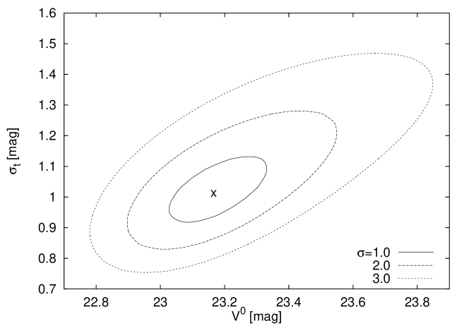
Figure 6: 1, 2, and $3\sigma$ contours for the fitted parameters $m^{0}$ and $\sigma_{t}$ in $V$ and $I$.

3.4.2 The TOM of the Galactic system

Although the Galactic TOM has been discussed by many authors, it is not a parameter that can be simply looked up in the literature. The exact value depends on the method of fitting, on the selection of GCs that enter the fitting process, on the distance scale of GCs, and on the exact application of a reddening law. Even if our values do not differ much from previous evaluations, we discuss them for numerical consistency.

We take the LMC distance as the fundamental distance for calibrating the zero-point in the relation between metallicity and horizontal branch/RR Lyrae brightness. The third fundamental distance determination beside trigonometric parallaxes and stellar stream parallaxes is the method of Baade-Wesselink parallaxes. It has been applied to the LMC in its modified form known as the Barnes-Evans method. So far, it has been applied to Cepheids in NGC 1866 (Gieren et al. gieren:94 (1994)), and the most accurate LMC distance determination to date stems from the period-luminosity relation of LMC Cepheids by Gieren et al. (gieren:98 (1998)). We adopt the distance modulus from the latter work, which is $18.46\pm 0.06$ mag, and which is in very good agreement with most other work (e.g. Tanvir tanvir:96 (1996)).

If we adopt the apparent magnitude of RR Lyrae stars in the LMC from Walker (walker:92 (1992)), $18.94\pm 0.1$ mag for a metallicity of $[\@element{\mathrm{Fe}}/\@element{\mathrm{H}}]=-1.9$ dex, and the metallicity dependence from Carretta et al. (carretta:99 (1999)), we find

$$M_{V}(RR)=(0.18\pm 0.09)([\@element{\mathrm{Fe}}/\@element{\mathrm{H}}]+1.6)+0.53\pm 0.12.$$ (8)

This zero-point is in excellent agreement with the value of $0.58\pm 0.12$ mag derived from HB-brightnesses of old LMC globular clusters from Suntzeff et al. (suntzeff:92 (1992)), if the above metallicity dependence is used. It also agrees within a one-$\sigma$ limit with $0.56\pm 0.12$ mag (Chaboyer chaboyer:99 (1999)) and $0.57\pm 0.04$ mag (Carretta et al. carretta:99 (1999)).

We calculate the absolute magnitudes of Galactic GCs from the McMaster catalogue (Harris harris:96 (1996)), using $A_{V}/E(B-V)=3.1$ (Rieke & Lebofsky rieke:85 (1985)) and $E(V-I)/E(B-V)=1.53$ (Ardeberg & Virdefors ardeberg:82 (1982)) as a compromise between the extreme values $1.6$ mag (Rieke & Lebofsky rieke:85 (1985)) and $1.35$ mag (Drukier et al. drukier:93 (1993)). We exclude clusters with $E(B-V)>1$ so that the sample embraces 120 clusters in $V$ and 93 in $I$.

Fig. 7 shows the scaled histograms ($V$ and $I$) for the sample of Galactic globular clusters. The solid line is the $t_{5}$-function resulting from the maximum-likelihood fit. It is not the fit to the histograms, which are shown just for visualisation purposes.

Figure 7: This graph shows the normalised distribution of absolute magnitudes in $V$ and $I$ for Galactic globular clusters. Overplotted as solid lines are the $t_{5}$-functions resulting from a maximum-likelihood fit. The bold histogram in the left panel shows the GCs with missing $I$-band photometry. The dotted vertical line denotes the cut-off magnitude at $m_{c}=-5.8$.

Figure 8: Dependence of the fitted $M_{V}^{0}$ (symbol ✕) and $\sigma_{t}$ (symbol $+$) on the cut-off magnitude $m_{c}$ for the Galactic GCS. The chosen $m_{c}=-5.8$ is indicated by the dashed line.

It is apparent from Fig. 7 that the symmetry in the $V$ distribution breaks down for clusters at the faint end of the distribution. It is reasonable to include in the fit only the symmetric part up to a certain limiting magnitude. To determine an appropriate cut-off magnitude $m_{c}$ we carry out the maximum-likelihood fit for various $m_{c}$ and look at how the fitted parameters evolve. Fig. 8 shows that the $V$-TOM $M^{0}_{V}$ and the width $\sigma_{t}$ clearly depend on $m_{c}$. The inclusion of the asymmetric part shifts $M_{V}^{0}$ systematically to greater values. This trend stops at our adopted value $m_{c}=-5.8$ mag and lowering $m_{c}$ further just results in a random scatter of $M_{V}^{0}$.

Table 4: Fitted TOMs and $\sigma_{t}$-values for the Galactic GC system. The $I$ values are biased due to selection effects as discussed in the text.

Filter	$M^{0}$	$\sigma_{t}$	# of GCs
$V$	$-7.61\pm 0.08$	$0.92\pm 0.07$	120
$I$	$-8.60\pm 0.07$	$0.85\pm 0.06$	93

There is no asymmetric part in the histogram of the $I$ band data in Fig. 7. The reason for this is a selection effect in the $I$ photometry. Looking at the McMaster catalogue data reveals missing $I$ data in approximately 22% of the listed GCs. All of these clusters with missing data belong to the fainter end of the luminosity function in $V$. This is shown by plotting the subset of GCs without $I$ magnitudes onto the $M_{V}$ histogram in Fig. 7. This incompleteness shifts the fitted $I$ TOM to brighter magnitudes. Thus, a comparison between the difference of the fitted TOMs and the mean colour of the Galactic GCs gives

$$0.87\pm 0.09=\langle V-I\rangle_{\mathrm{MW}}<M_{V}^{0}-M_{I}^{0}=1.01\pm 0.11.$$ (9)

The median is equal to the mean of the $V-I$ distribution for the Galactic GCs. We therefore use

$$M_{I}^{0}=M_{V}^{0}-\langle V-I\rangle_{\mathrm{MW}}=-8.48\pm 0.10$$ (10)

as an absolute TOM in the $I$ band. Alternatively, we introduce a cut-off magnitude in the $I$ band data and fit only the more complete luminous part of the distribution like we did in the $V$ band. As expected, the fitted $I$ TOM becomes smaller with decreasing cut-off magnitude. If the cut-off magnitude approaches the TOM the fitted TOM values begin to scatter greatly around approximately $-8.52$ mag because the sample size decreases and the fit results are less well determined. We therefore do not rely on this approach but rather regard it as a confirmation of the validity of (10).

3.5 Metallicity correction and distance

The luminosity of a GC depends not only on its mass but also on its metallicity. Any difference between the metallicities of the GCS of NGC 4526 and the Galactic GCS must be corrected to avoid a systematic bias.

The amount of this correction has been studied by Ashman et al. (ashman:95 (1995)) and we adopt their values. The only metallicity indicator that is available for us is the mean $V-I$ colour of the GCS, for which we adopt the relation given by Couture et al. (couture:90 (1990)):

$$V-I=0.2\cdot[\@element{\mathrm{Fe}}/\@element{\mathrm{H}}]+1.2.$$ (11)

A mean colour of $\langle V-I\rangle=1.1$ indicates $[\@element{\mathrm{Fe}}/\@element{\mathrm{H}}]_{\mathrm{NGC4526}}=-0.5\pm 0.3$ and we find a metallicity correction of $\Delta M_{V}^{0}=0.28\pm 0.19$ and $\Delta M_{I}^{0}=0.11\pm 0.05$. The large error of $\pm 0.3$ dex for the metallicity arises from the fact that $\langle V-I\rangle$ depends only weakly on the metallicity. This value can be estimated from looking at the scatter in the $[\@element{\mathrm{Fe}}/\@element{\mathrm{H}}]$–$(V-I)$ plot of the Galactic GCS.

Hence the distance moduli in $V$ and $I$ are

$$\mu_{V}=30.49\pm 0.26\quad\mbox{and}\quad\mu_{I}=30.33\pm 0.14.$$ (12)

If the universality of the TOM of $\approx 0.2$ mag (Whitmore whitmore:97 (1997)) and the uncertainty in the horizontal branch calibration of $\approx 0.1$ mag is included as external errors we obtain

$$\mu_{\mathrm{NGC4526}}=30.4\pm 0.3\,\mbox{mag}$$ (13)

and

$$D_{\mathrm{NGC4526}}=12.0\pm 1.6\,\mbox{Mpc}$$ (14)

as our final value for the distance modulus and distance.

Thus, NGC 4526 is located in the foreground of the Virgo cluster and a comparison with apparent magnitudes of other SNe in the Virgo cluster is misleading. This result is consistent within $1\sigma$ with Tonry’s unpublished SBF distance modulus $30.68\pm 0.13$ mag, which was used by Richmond et al. (richmond:95 (1995)).

4 Comparison with other supernovae

4.1 The dependence on decline rate and colour

The publication of the Calán/Tololo-sample of Ia SNe (Hamuy et al. hamuy:96 (1996)) confirmed in a compelling way what has been suggested earlier, namely that the luminosity of Ia’s depends on the decline rate and also on the colour of the SN at maximum phase.

Here we report convenient expressions which relate in the sample of Hamuy et al. the decline rate $\Delta m_{15}$ and the foreground extinction-corrected colour $B_{\mathrm{max}}-V_{\mathrm{max}}$ with the apparent maximum magnitude (the recently published sample by Riess et al. (riess:98 (1998)) does not change significantly the numerical values). These linear relations read

$$\begin{array}[]{l}m_{\mathrm{max},i}+b\cdot(\Delta m_{15}-1.1)+R\cdot(B_{\mathrm{max}}-V_{\mathrm{max}})\\ \leavevmode\nobreak\ =5\cdot\log cz+Z\end{array}$$ (15)

where $i\in\{B,V,I\}$ denotes the different bands. Table 5 lists the coefficients, which have been obtained by a maximum-likelihood fit, together with their errors. Only SNe with $B_{\mathrm{max}}-V_{\mathrm{max}}<0.2$ have been used for the fit. Fig. 9 shows the relation between $B_{\mathrm{max}}-V_{\mathrm{max}}$ and the apparent maximum brightness corrected for decline rate. The fact that the red SNe are also well fitted by this relation indicates the validity of this relation for a larger colour range. The coefficients of the colour term also deviate strongly from the Galactic reddening law so that one may conclude that the red colours are indeed intrinsic and not significantly affected by reddening.

Figure 9: This plot shows the relation between $B_{\mathrm{max}}-V_{\mathrm{max}}$ rate and the apparent maximum brightness in $B$ corrected for the decline rate. A clear dependence is visible. We point out that only blue SNe with $B_{\mathrm{max}}-V_{\mathrm{max}}<0.2$ have been included in the fit. The fact that the redder SNe are well represented by this relation is a point in favour of the validity of this relation even over a larger colour range.

The corrected magnitudes can now be compared with those of other SNe.

Table 5: The table lists the coefficients according to (15) for the relation between brightness, decline rate, and colour for the Calán/Tololo sample.

Band	$Z$	$b$	$R$
$B$	$-3.306\pm 0.063$	$-0.48\pm 0.23$	$-1.51\pm 0.62$
$V$	$-3.320\pm 0.058$	$-0.52\pm 0.19$	$-0.83\pm 0.57$
$I$	$-3.041\pm 0.060$	$-0.40\pm 0.22$	$-0.81\pm 0.59$

4.2 Comparison with other SNe

Table 6: The observational data and distance moduli of the SNe. The first three rows show the extinction-corrected apparent magnitudes computed with $A_{B}/E(B-V)=4.09$, $A_{V}/E(B-V)=3.09$ and $A_{I}/E(B-V)=1.49$ (Rieke & Lebofsky rieke:85 (1985)). Photometric data, colour excesses and decline rates are taken from Richmond et al. (richmond:95 (1995)) for SN 1994D, from Hamuy et al. (hamuy:96 (1996)) for SN 1992A and SN 1980N, and from Hamuy et al. (hamuy:91 (1991)) for SN 1981D. The absolute magnitudes are corrected for decline rate and colour by (15).

	SN 1994D	SN 1992A	SN 1980N	SN 1981D
$B_{\mathrm{max}}$	$11.73\pm 0.02$	$12.57\pm 0.03$	$12.49\pm 0.03$	$12.59$
$V_{\mathrm{max}}$	$11.78\pm 0.02$	$12.55\pm 0.03$	$12.44\pm 0.03$	$12.40$
$I_{\mathrm{max}}$	$12.00\pm 0.05$	$12.80\pm 0.03$	$12.70\pm 0.04$	—
$\Delta m_{15}(B)$	$1.31\pm 0.08$	$1.47\pm 0.05$	$1.28\pm 0.04$	—
$B_{\mathrm{max}}-V_{\mathrm{max}}$	$-0.05\pm 0.04$	$0.02\pm 0.04$	$0.05\pm 0.04$	$0.19$
$E(B-V)$	$0.04\pm 0.03$	$0$	$0$	$0$ (?)
$\mu$	$30.40\pm 0.30$	$31.35\pm 0.15$	$31.35\pm 0.15$	$31.35\pm 0.15$
$M_{B,\mathrm{cor}}$	$-18.69\pm 0.31$	$-18.99\pm 0.16$	$-19.02\pm 0.16$	—
$M_{V,\mathrm{cor}}$	$-18.69\pm 0.31$	$-19.01\pm 0.16$	$-19.04\pm 0.16$	—
$M_{I,\mathrm{cor}}$	$-18.44\pm 0.31$	$-18.69\pm 0.16$	$-18.74\pm 0.16$	—

A meaningful comparison of SN 1994D with other SNe requires the distances of the comparison objects to be derived with the same method of GCLFs, because then the comparison is valid without the need for an absolute calibration of GCLFs. Moreover, these SNe should be well observed. These two conditions are fulfilled only in the Fornax galaxy cluster with its 3 Ia SNe SN 1980N, SN 1981D (both in NGC 1316), and SN 1992A (in NGC 1380). The light curves of the first two SNe have been presented by Hamuy et al. (hamuy:91 (1991)), while SN 1992A (one of the best observed SNe) is described by Suntzeff (suntzeff:96 (1996)).

All these SNe are relatively fast decliners, and thus follow the trend already visible in the Calán/Tololo SN sample (Hamuy et al. hamuy:96 (1996)) that spiral galaxies host all kinds of SNe, while early-type galaxies tend to host only fast decliners (which are intrinsically fainter).

The Fornax cluster is well suited to serve as a distance standard. It is compact with hardly any substructure and consists in its core region almost entirely of ellipticals and S0 galaxies, the characteristics of a well relaxed galaxy cluster. The distance based on GCLFs has been determined through the work of Kohle et al. (kohle:96 (1996)) and Kissler-Patig et al. (1997a ), who analysed the GCSs for several early-type galaxies. In addition, Kissler-Patig et al. (1997b ) and Della Valle et al. (dellavalle:98 (1998)) determined the luminosity function for the GCS of NGC 1380, host of SN 1992A. Kohle et al. (kohle:96 (1996)) derived mean apparent TOMs for their sample of 5 Fornax galaxies of $V^{0}=23.67\pm 0.06$. This is in perfect agreement with the TOM of NGC 1380 given by Della Valle et al. (dellavalle:98 (1998)), which is $V^{0}=23.67\pm 0.11$. The difference in distance moduli between Kohle et al. (kohle:96 (1996)) and Della Valle et al. (dellavalle:98 (1998)) stems from a revised absolute TOM of the Galactic GCS. If this is based on the Gratton et al. (gratton:97 (1997)) relation, which is similar to our eq. (8), the distance modulus is $\mu_{\mathrm{Fornax}}=31.35\pm 0.15$ mag. It is very satisfactory that several other independent methods confirm our distance estimate (Richtler et al. richtler:99b (1999)). For example, Madore et al. (madore:98 (1998)) recently published a Cepheid distance to NGC 1365 and quoted $31.35\pm 0.2$ mag. Moreover, the method of surface brightness fluctuations gives a Fornax distance modulus of $31.32\pm 0.24$ mag (Jensen et al. jensen:98 (1998)).

For the other host galaxy in Fornax, NGC 1316, no published GCLF distance exists. Grillmair et al. (grillmair:99 (1999)), using HST data, found no turn-over but an exponential shape of the GCLF. They explained this with a population of open clusters mixed in, presumably dating from the past merger event. Preliminary results from ongoing work (Gómez et al., in preparation), however, place the TOM of the entire system at the expected magnitude, but indicate a radial dependence in the sense that the TOM becomes fainter at larger radii. At this moment, we have no good explanation. Perhaps, the different findings correspond to the different regions in NGC 1316 investigated. This issue is not yet settled.

An individual distance value for NGC 1316 based on planetary nebulae seems to indicate a shorter distance to this galaxy than to the Fornax cluster. McMillan et al. (mcmillan:93 (1993)) find $\mu_{\mathrm{PN,NGC\,1316}}=31.13$ mag, but this value is based on a M31 distance modulus of $24.26$ mag. Adopting the now widely accepted M31 Cepheid distance modulus of $24.47$ mag (e.g. Stanek & Garnavich stanek:98 (1998), Kochanek kochanek:97 (1997)), the NGC 1316 modulus increases to $31.34$ mag, perfectly consistent with the global Fornax distance. We therefore adopt the Fornax distance modulus of $\mu_{\mathrm{Fornax}}=31.35\pm 0.15$ mag for SN 1992A and SN 1980N.

Table 6 lists the absolute magnitudes of SN 1994D together with two Fornax cluster SNe (SN 1981D was badly observed), corrected for decline-rate and colour. All values can be derived from the photometric data and distances shown in table 6 together with our correction equation (15).

One notes that SN 1994D seems to be 0.3 mag too faint in all three photometric bands. However, the error bars overlap with those of the other SNe. Thus, there is no reason to claim that this SN is peculiarly dim. On the other hand, if one takes Tonry’s unpublished SBF distance modulus, which is 0.28 mag greater than ours, all three SNe brightnesses would agree within $\pm 0.05$ mag. At any rate, it is apparent that SN 1994D is definitely not overluminous and cannot be taken for a counter-example against the general validity of the decline-rate–colour–luminosity relation.

4.3 The Hubble constant

Once the absolute brightness of a supernova is known, the Hubble diagram of SNe Ia (Hamuy et al. hamuy:96 (1996)) allows the derivation of the Hubble constant with an accuracy which is largely determined only by the error in the supernova brightness. The fact that the Fornax SNe are well observed in combination with a reliable distance makes these objects probably the best SNe for this purpose. The relation between the Hubble constant, the absolute corrected magnitude $M$ and the zero-point $Z$ in (15) reads

$$\log\frac{H_{0}}{\mathrm{km\,s^{-1}\,Mpc^{-1}}}=0.2\cdot(M-Z)+5.$$ (16)

Taking the data from SN 1994D, SN 1992A, and SN 1980N presented in Table 6 and the zero-points from Table 5 yields a Hubble constant of

$$H_{0}=75\pm 6\pm 6\,\mathrm{km\,s^{-1}\,Mpc^{-1}}.$$ (17)

The systematic error originates from the horizontal branch magnitude, the universality of the TOM, the adopted Fornax distance and the error in $Z$. The statistical error is just the scatter from the three corrected SNe absolute magnitudes. This Hubble constant value is dominated by the data from the Fornax SNe because of the small statistical weight of SN 1994D.

5 Summary

We determined the GCLF distance of NGC 4526 to be $12.0\pm 3.9$ Mpc, placing this galaxy in front of the Virgo cluster. Although this distance is not precise enough to give a good absolute magnitude it is sufficient to show that SN 1994D is not an overluminous type Ia SN but rather a normally bright event compared to the two Fornax SNe SN 1992A and SN 1980N.

All GCLF distances depend on the absolute luminosities of the Galactic GCs. It is therefore vital to calibrate the absolute TOM properly to minimise systematic errors. The most important calibration parameter is the absolute magnitude of the horizontal branch which directly enters our distance scale. The treatment of the Galactic GC sample shows that the asymmetric distribution in $V$ and incompleteness effects in the $I$ band can introduce a bias in the TOM of over $0.1$ mag.

With the distances and the apparent decline-rates and colour-corrected magnitudes of the three SNe SN 1994D, SN 1982A, and SN 1980N one obtains an absolute corrected peak magnitude of type Ia SNe. The Calán/Tololo SN sample gives us the zero-point of the Hubble diagram, the second ingredient in calculating the Hubble constant from type Ia SNe. Our data give $H_{0}=75\pm 6(\mbox{sys.})\pm 6(\mbox{stat.})\,\mathrm{km\,s^{-1}\,Mpc^{-1}}$.