Effects of cluster galaxies on arc statistics

Abstract

We present the results of a set of numerical simulations evaluating the effect of cluster galaxies on arc statistics.

We perform a first set of gravitational lensing simulations using three independent projections for each of nine different galaxy clusters obtained from N-body simulations. The simulated clusters consist of dark matter only. We add a population of galaxies to each cluster, mimicking the observed luminosity function and the spatial galaxy distribution, and repeat the lensing simulations including the effects of cluster galaxies, which themselves act as individual lenses. Each galaxy is represented by a spherical Navarro, Frenk & White (1997) density profile.

We consider the statistical distributions of the properties of the gravitational arcs produced by our clusters with and without galaxies. We find that the cluster galaxies do not introduce perturbations strong enough to significantly change the number of arcs and the distributions of lengths, widths, curvature radii and length-to-width ratios of long arcs. We find some changes to the distribution of short-arc properties in presence of cluster galaxies. The differences appear in the distribution of curvature radii for arc lengths smaller than $12^{\prime\prime}$, while the distributions of lengths, widths and length-to-width ratios are significantly changed only for arcs shorter than $4^{\prime\prime}$.

1 Introduction

Strong gravitational lensing by galaxy clusters distorts the images of galaxies in the background of the clusters and thereby gives rise to the formation of giant luminous arcs near the cluster cores. Bartelmann et al. (1998) showed recently that the statistics of arcs is a potentially very sensitive probe for the cosmological matter density parameter $\Omega_{0}$ and for the contribution $\Omega_{\Lambda}$ to the total density parameter due to the presence of the cosmological constant. The reason can be summarised in form of three statements. (i) Typical arc sources are located at redshifts around unity. Lenses have to be placed approximately half-way between the sources and the observer in order to be efficient, namely at redshifts around $0.3$. (ii) The formation and evolution of galaxy clusters depends strongly on the cosmological model (Richstone, Loeb & Turner 1992; Bartelmann, Ehlers & Schneider 1993). They tend to form only recently in high-density universes and early in low-density universes. In order to have a population of galaxy clusters capable of forming arcs, at least a sufficiently large fraction of them must have formed by redshift $\sim 0.3$ because of argument (i). (iii) The density of cluster cores depends on the formation redshift of the clusters (Navarro, Frenk & White 1996, 1997). The earlier a cluster forms, the more compact it is. In universes with low density, clusters therefore tend to be less compact the higher the cosmological constant is.

Taken together, these arguments imply that more arcs can be observed in a universe with low density and small cosmological constant: low density makes clusters form earlier, and a low cosmological constant makes them more compact individually.

This line of reasoning can easily be supported using Press-Schechter (1974) theory. Numerical cluster simulations are necessary for quantitative statements. They lead to the result that the number of (suitably defined) large arcs on the whole sky is of order $10$ in an Einstein-de Sitter universe, of order $100$ in a spatially-flat, low-density universe with $\Omega_{0}=0.3$, and of order $1,000$ for an open model with the same $\Omega_{0}$ and $\Omega_{\Lambda}=0$. The observed number of arcs, which is of order $1,000$ when extrapolated to the whole sky, then leads to the conclusion that $\Omega_{0}$ should be low and $\Omega_{\Lambda}$ should be small or zero.

This result is important for several reasons. First, the effect is in principle easy to observe. It “only” requires to count arcs in a sufficiently large portion of the sky above a certain brightness, which are distorted by a certain minimum amount. Second, the effect is strong because order-of-magnitude differences are expected across certain popular cosmological models. Third, the consequence that $\Omega_{\Lambda}$ should be small or zero is at odds with the results obtained by the recent searches for supernovae of type Ia, which indicate that the universe is most likely spatially flat and has low density (Perlmutter et al. 1999).

The previous study (Bartelmann et al. 1998) neglected the granularity of the gravitational cluster potentials. It was ignored that the cluster galaxies could influence the lensing properties of clusters. Cluster galaxies have two principal effects. First, they tend to wiggle the critical curves of the cluster lenses, thereby increasing their lengths, and thus also the cross sections for strong lensing. Second, the larger local curvature of the critical curves can cause long arcs to split up, so that several shorter arcs can be formed where one long arc would have been formed in absence of the perturbing galaxies. These effects are counter-acting, and it requires numerical simulations to quantify their net effect. A secondary effect is that the local steepening of the density profile near cluster galaxies tends to make arcs thinner.

We present in this paper numerical experiments to quantify the effect of cluster galaxies on the cross sections for formation of large arcs. In particular, we address the question whether lensing by cluster galaxies can invalidate the earlier result that clusters in a high-density universe fail by two orders of magnitude to produce the observed number of arcs. We describe the cluster simulations and the technique used to study the lensing properties of the clusters in Section 2. The procedure for putting galaxies into them is presented in Section 3 where we also describe the method followed to compute the deflection angles. The technique for identifying arcs and the results about the distributions of their properties are detailed in Section 4. We finish with a summary and a discussion in Section 5.

2 The numerical method

2.1 The cluster sample

The simulated clusters used as lenses in the present analysis are those presented by Tormen, Bouchet & White [1997]. We will only briefly describe them here and refer to that paper for more details.

The sample is formed by the nine most massive clusters obtained in a cosmological simulation of an Einstein-de Sitter universe, evolved using a particle-particle-particle-mesh code. The initial conditions have a scale-free power spectrum $P(k)\propto k^{-1}$, very close to the behaviour of the standard Cold Dark Matter model on the scales relevant for cluster formation. Despite the scale-free power spectrum, a size can be assigned to the simulation box by determining the variance of the dark-matter fluctuations and fixing the scale such that the variance matches a certain value on that scale. Accordingly, we demand that the rms density fluctuation in spheres of radius $r=8\,h^{-1}\;$Mpc is $\sigma_{8}=0.63$, in rough agreement with the normalisation of the power spectrum required to match the observed local abundance of clusters [1993]. The comoving size of the simulation box then turns out to be $L=150\;$Mpc (in this paper a Hubble constant of $50\,{\rm km\,s^{-1}\,Mpc^{-1}}$ is used).

Each cluster was obtained using a re-simulation technique (e.g. Tormen et al. 1997). In short, for each cluster in the cosmological simulation new initial conditions were set up, in which the cluster Lagrangian region was sampled by a higher number of particles than in the original run. This allows a much higher spatial and mass resolution in the re-simulated cluster. Particles not contributing to the cluster were interpolated on a coarser distribution, which describes the correct large-scale tidal field. These initial conditions were evolved until the final time using a tree/SPH code [1993], without gas, i.e. as a pure N-body code.

Some of the cluster properties are summarised in Table 1. Virial masses, encompassing an average overdensity $\delta\rho/\rho=178$, range from $M_{\rm vir}=5.32\times 10^{14}\,M_{\odot}$ to about $3\times 10^{15}\,M_{\odot}$, while one-dimensional rms velocities within the virial radius $R_{\rm vir}$ range from 700 to 1300 km s^-1. The average number of particles within a cluster’s $R_{\rm vir}$ is $\simeq 20,000$. The gravitational softening $s$ imposed on small scales follows a cubic spline profile, and was kept fixed in physical coordinates. Its value is $s=20-25$ kpc at the final time, depending on the simulation. Consequently, the force resolution in the simulations is $L/s\simeq 6,000$ to $7,500$ for the box and of the order of $R_{\rm vir}/s\simeq 100$ for each cluster.

Table 1: Main properties of the simulated clusters. Column 1: cluster name; column 2: average number of particles inside the virial radius; column 3: virial mass; column 4: virial radius; column 5: one-dimensional rms velocity within $R_{\rm vir}$.

Cluster	$N_{\rm vir}$	$M_{\rm vir}$		$R_{\rm vir}$	$v_{\rm rms}$
name		[$M_{\odot}$]		[kpc]	[km s-1]
g15	39400	$2.99$$\times$	$10^{15}$	3870	1260
g23	17400	$6.76$$\times$	$10^{14}$	2350	750
g36	18200	$1.51$$\times$	$10^{15}$	3070	1000
g40	21300	$5.32$$\times$	$10^{14}$	2170	730
g51	23500	$1.38$$\times$	$10^{15}$	2990	1000
g57	24400	$7.01$$\times$	$10^{14}$	2380	780
g66	21400	$1.10$$\times$	$10^{15}$	2770	920
g81	14400	$7.05$$\times$	$10^{14}$	2390	750
g87	16200	$6.21$$\times$	$10^{14}$	2290	740

2.2 Lensing properties of the clusters

To study the lensing properties of a cluster, we first define a three-dimensional density field as follows. We centre the cluster in a cube of $6$ Mpc side length, which is covered with a regular grid of $N_{\rm g}=128^{3}$ cells. The resolution of the grid is therefore $R=6\,{\rm Mpc}/{N_{\rm g}^{1/3}}\approx 47$ kpc. The three-dimensional cluster density $\rho$ at the grid points is calculated with the Triangular Shape Cloud method (see Hockney & Eastwood 1988), which allows to avoid discontinuities. We extracted three different surface-density fields $\Sigma$ from each cluster by projecting $\rho$ along the three coordinate axes. This gives three lens planes per cluster which we consider independent cluster models for our present purpose. We can thus perform 27 different lensing simulations starting from our sample of nine clusters.

We find the convergence $\kappa$ by dividing the projected density fields $\Sigma$ with the critical surface mass density for lensing, defined as

$$\Sigma_{\rm cr}\equiv\frac{c^{2}}{4\pi G}\frac{D_{\rm S}}{D_{\rm L}D_{\rm LS}}\ ,$$ (1)

where $c$ is the speed of light, $G$ is the gravitational constant and $D_{\rm L}$, $D_{\rm S}$ and $D_{\rm LS}$ are the angular-diameter distances between lens and observer, source and observer, and lens and source, respectively. We adopt $z_{\rm L}=0.4$ and $z_{\rm S}=2$ for the lens and source redshifts in the following. Hence,

$$\Sigma_{\rm cr}\approx 2\times 10^{15}\,\frac{M_{\odot}}{{\rm Mpc}^{2}}\ .$$ (2)

Although real source galaxies are distributed in redshift, putting them all at a single redshift is permissible because the critical surface mass density (eq. 1) changes only very little with source redshift if the sources are substantially more distant than the lensing cluster.

We further scale lens-plane coordinates with an arbitrary length $\xi_{0}$, and source plane coordinates with the projected length $\eta_{0}\equiv D_{\rm S}/D_{\rm L}\,\xi_{0}$. The lens equation can then be written

$$\vec{y}=\vec{x}-\alpha(\vec{x})\ ,$$ (3)

with the reduced deflection angle

$$\vec{\alpha}(\vec{x})=\frac{1}{\pi}\,\int\frac{\kappa(\vec{x}^{\prime})\,(\vec{x}-\vec{x}^{\prime})}{|\vec{x}-\vec{x}^{\prime}|^{2}}\,{\rm d}^{2}\vec{x}^{\prime}\ .$$ (4)

Aiming at the simulation of large arcs, we can concentrate on the cluster centres, i.e. on the central regions of each lens plane. We therefore propagate a bundle of $1024\times 1024$ light rays only through the central quarter of each lens plane. The corresponding resolution of this grid of rays is then fairly high, $\sim 3$ kpc.

The deflection angle $\vec{\alpha}_{ij}$ of each light ray ($i,j$) is calculated with the discretised eq. (4). Recall that the convergence is defined on a grid, $\kappa_{mn}$, with $m,n=1,\ldots,128$. We thus have

$$\vec{\alpha}_{ij}=\frac{1}{\pi}\,\sum\limits_{m,n}\,\frac{\kappa_{mn}(\vec{x}_{ij}-\vec{x}_{mn})}{|\vec{x}_{ij}-\vec{x}_{mn}|}\ ,$$ (5)

where $\vec{x}_{ij}$ and $\vec{x}_{mn}$ are the positions on the lens plane of light ray ($i,j$) and grid point ($m,n$). The deflection angles could diverge when the distance between a light ray and the density grid-point is zero. Following Wambsganss, Cen & Ostriker [1998], we avoid this divergence by first calculating the deflection angle on a regular grid of $128\times 128$ “test rays”, shifted by half-cells in both directions with respect to the grid on which the surface density is given. We then determine the deflection angle of each light ray by bicubic interpolation between the four nearest test rays.

The local properties of the lens mapping are described by the Jacobian matrix of the lens equation (3),

$$A_{hk}(\vec{x})\equiv\frac{\partial{y}_{h}}{\partial{x}_{k}}=\delta_{hk}-\frac{\partial\alpha_{h}}{\partial x_{k}}\ .$$ (6)

The shear components $\gamma_{1}$ and $\gamma_{2}$ are found from $A_{hk}$ through the standard relations

$$\gamma_{1}(\vec{x}) = -\frac{1}{2}\left[A_{11}(\vec{x})-A_{22}(\vec{x})\right]\ ,$$ (7)

$$\gamma_{2}(\vec{x}) = -\frac{1}{2}\left[A_{12}(\vec{x})+A_{21}(\vec{x})\right]\ ,$$ (8)

and the magnification factor is given by the Jacobian determinant,

$$\mu(\vec{x})=\frac{1}{\det A}=[A_{11}(\vec{x})A_{22}(\vec{x})-A_{12}(\vec{x})A_{21}(\vec{x})]^{-1}\ .$$ (9)

Finally, the Jacobian determines the location of the critical curves $\vec{x}_{\rm c}$ on the lens plane, which are defined by $\det A(\vec{x}_{\rm c})=0$. Because of the finite grid resolution, we can only approximately locate them by looking for pairs of adjacent cells with opposite signs of $\det A$. The corresponding caustics $\vec{y}_{\rm c}$ on the source plane are given through the lens equation,

$$\vec{y}_{\rm c}=\vec{x}_{\rm c}-\vec{\alpha}(\vec{x}_{\rm c})\ .$$ (10)

3 Inserting cluster galaxies

The goal of this paper is to evaluate the effects of cluster galaxies on arc statistics. For this purpose, we need to simulate a population of galaxy lenses inside the cluster, in such a way that their observational properties are well reproduced.

3.1 Galaxy distribution

We start with the galaxy luminosity function. It is widely accepted that the faint-end slope of the luminosity function depends on the environment. In particular, it is steeper for cluster galaxies than for field galaxies (Bernstein et al. 1995; De Propris et al. 1995). Using a catalogue of isophotal magnitudes in the V band for 7,023 galaxies, Lobo et al. [1997] derived the luminosity function in the Coma cluster in the magnitude range $13.5<V\leq 21.0$ (corresponding to the absolute magnitude range $-22.24<M_{V}\leq-14.74$). Their results were fitted using both a steep Schechter function,

$$S(M_{V})=K_{\rm S}\,10^{0.4(\alpha+1)(M_{V}^{*}-M_{V})}\exp[-10^{0.4(M_{V}^{*}-M_{V})}]$$ (11)

(hereafter case “S”), and a 4-parameter combination of a Schechter function with a Gaussian,

$$G(M_{V})=K_{\rm G}\,\exp[-(M_{V}-\mu)^{2}/(2\sigma^{2})]\ ,$$ (12)

on its bright end (hereafter case “S+G”). After excluding the three brightest cluster members, they found $M^{*}_{V}=-29.0\pm 2.0$ and $\alpha=-1.59\pm 0.02$ (with reduced $\chi^{2}=3.1$) in the “S” case, while a much better fit (with $\chi^{2}=0.6$) was achieved in the “S+G” case, with parameters $M^{*}_{V}=-22.7\pm 0.4$, $\alpha=-1.80\pm 0.05$, $\mu=-20.4\pm 0.2$ and $\sigma=1.1\pm 0.3$.

Notice that the Coma cluster has a mass similar to our simulated clusters. In fact, Vedel & Hartwick [1998] recently estimated that the mass of Coma within a radius of 5 Mpc falls in the range $2.2-4.8\times 10^{15}M_{\odot}$. We apply the two luminosity functions from Lobo et al. [1997] to all our simulated galaxy clusters.

Galaxy luminosities $L$ can be converted to baryonic masses $M$ with the relation

$$\frac{M}{L}=4.0\,\left(\frac{L}{4\times 10^{10}\,L_{\odot}}\right)^{0.35}\,\left(\frac{M_{\odot}}{L_{\odot}}\right)\ ,$$ (13)

derived by van der Marel [1991] from a study of a sample of 37 elliptical galaxies. White et al. [1993] found $\langle M/L\rangle=3.2(M_{\odot}/L_{\odot})$ by averaging this relation over a luminosity function similar to that of the Coma cluster.

Using the previous relations in Monte Carlo methods, we can now generate a sample of galaxies with luminosities (and masses) distributed like the galaxies in Coma. We will only consider galaxies with a baryonic mass corresponding to the magnitude range where the Lobo et al. (1997) data were fit; this corresponds to a range $8.6\times 10^{8}\,M_{\odot}<M<8.6\times 10^{11}\,M_{\odot}$. In order to be fully consistent with Lobo et al. (1997), we include in our simulated sample three more objects with luminosities (and masses) corresponding to those of the three galaxies excluded from their analysis.

The total number of galaxies to be placed in each simulated cluster is determined by imposing a baryonic fraction as observed in Coma. We adopt the estimate of White et al. [1993], who found a ratio between the baryonic mass in galaxies $M_{\rm b}$ and the total mass of the cluster $M_{\rm tot}$ within the Abell radius $M_{\rm b}/M_{\rm tot}\simeq 0.009$.

Finally, we must account for dark-matter haloes encompassing each galaxy. We calculate total (virial) halo masses $M_{\rm vir}$ by multiplying the baryonic masses $M_{\rm b}$ with the factor $f_{\rm b}^{-1}$, where $f_{\rm b}$ is the average baryon fraction within individual galaxies. Since this factor is not well known observationally, we take a fiducial value of $f_{\rm b}\sim 5\%$. This number is close to the baryon fraction predicted by the standard model of primordial nucleosynthesis.

The right panel of Figure 1 shows the distribution of galaxy virial masses $M_{\rm vir}$ in our most massive cluster (g15), using both luminosity functions “S+G” and “S” with the best-fit parameters from Lobo et al. [1997]. The obvious main difference between the two cases is that the number of massive galaxies is larger for the “S+G” luminosity function. The total number of galaxies is therefore larger when the luminosity function “S” is adopted, where the same total mass is distributed over a larger number of less massive galaxies.

Notice that the more massive a galaxy is, the stronger is the perturbation caused by its potential. Therefore, the effect of cluster galaxies on arc statistics will be more pronounced when the luminosity function “S+G” is used.

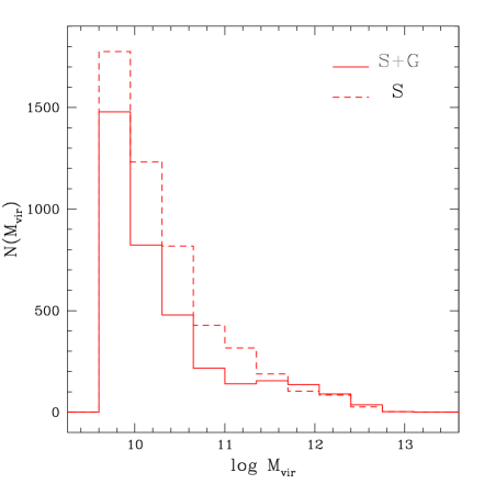
Figure 1: Histograms of galaxy virial masses $M_{\rm vir}$ (left panel) and of truncated masses $M_{\rm t}$ (right panel) for the simulated sample of galaxies in cluster g15. Masses are in units of $M_{\odot}$. The solid and dashed lines are for the “S+G” and “S” luminosity functions, respectively.

We would like the galaxy number density to follow the mass density, i.e. galaxies should preferentially be positioned in overdense regions. Furthermore, the most massive galaxies should be placed near the centre of the cluster and in other large sublumps, i.e. near the highest density peaks. We achieve this by assigning to any given position inside the cluster a probability for placing a galaxy which is linearly proportional to the local density of dark matter.

Using a Monte Carlo technique, we first compute the number of galaxies expected in each of the $32^{3}$ cells of a regular cubic grid covering the cluster. Since the dark matter density was earlier defined on a $128^{3}$ grid, each of these cells corresponds to $4^{3}$ cells of the density grid, and contains a sufficient mass to host a galaxy.

We then sort the galaxy catalogue by decreasing mass, and start to distribute them among the big cells with a probability proportional to the local galaxy number density. This ensures that massive galaxies are preferentially being placed in massive cells. Each galaxy is finally randomly shifted within its grid cell.

3.2 Galaxy mass profiles

Navarro, Frenk & White [1997] (hereafter NFW) found that the equilibrium density profile of dark-matter haloes formed in numerical simulations of several cosmological models (including most CDM-like ones) is very well described by the radial function

$$\frac{\rho_{{}_{\rm NFW}}(r)}{\rho_{\rm cr}}=\frac{\delta_{\rm c}}{(r/r_{\rm s})(1+r/r_{\rm s})^{2}}\ ,$$ (14)

where $\delta_{\rm c}$ is a characteristic (dimension-less) density and $r_{\rm s}$ is the scale radius; $\rho_{\rm cr}$ is the critical density. We adopt this mildly singular density profile for our simulated galaxies. Navarro et al. [1997] also showed that the parameters $r_{\rm s}$ and $\delta_{\rm c}$ depend only on the virial mass of a halo. Using the definition of the virial radius, they are linked by the simple relation

$$\delta_{\rm c}=\frac{200}{3}\frac{k^{3}}{[\ln(1+k)-k/(1+k)]}\ ,$$ (15)

where the halo concentration $k$ is defined as the ratio between the virial radius $r_{\rm vir}$ and the scale radius $r_{\rm s}$.

We truncate each galaxy at a cut-off radius $r_{\rm t}$ where the galaxy density falls below the local cluster density. If we call $D$ the distance of the centre of the galactic halo from the cluster centre and $\rho$ is the cluster density profile, the cut-off radius $r_{\rm t}$ is determined by solving the equation

$$\rho_{{}_{\rm NFW}}(r_{\rm t})=\rho(D-r_{\rm t})\ .$$ (16)

Knowing position and radius of each galaxy, we can determine what mass must be subtracted from each small cell in exchange for the galaxy mass. This is done via a Monte Carlo integration. The histogram of the truncated galaxy masses $M_{\rm t}$ obtained for cluster g15 considering both luminosity functions is shown in the left panel of Fig. 1.

To avoid that all the galaxies concentrate near the cluster centre, we impose that the cluster baryonic fraction is $\sim 0.9\%$ also locally in each “large” cell. This implicitly means that we assume that the relative concentration of mass and stars is similar in all regions of the clusters without spatial segregation.

An example of a galaxy distribution obtained with this positioning procedure is shown in Fig. 2. All plots refer to cluster g15 and show results for the two different luminosity functions “S+G” and “S”. Each galaxy is represented in the figure by a circle of radius $r_{\rm t}$, and it is superimposed on the cluster convergence map, which is proportional to the surface mass density. Galaxies near the cluster centre have a smaller radius $r_{\rm t}$ because the cluster density is higher there, so only a small part of the galaxy profile emerges above the cluster.

Figure 2: Galaxy positions in cluster g15. Results for the two different luminosity functions “S+G” and “S” are shown in the left and right panels, respectively. Each galaxy is drawn as a circle with radius equal to its truncated radius $r_{\rm t}$. Both panels also show the convergence map. The scale of the figure is 3 Mpc on a side, which corresponds to an angular dimension of $\simeq 333^{\prime\prime}$ for a cluster placed at $z_{\rm L}=0.4$.

Figure 3 displays the distribution of virial and truncated galaxy masses as a function of their distance from the cluster centre $d$. In the right panel the distribution of the ratios $M_{\rm t}/M_{\rm vir}$ is also presented. The median and the upper and lower quartiles of the distributions are shown by solid and dashed lines, respectively. The use of different luminosity functions does not change the results significantly. For this reason, we will only show results for the “S+G” luminosity function here and in the rest of this paper, as it fits the Coma cluster data more accurately. The plots show that the most massive galaxies are either near the cluster centre or in secondary clumps at a distance of 2-3 Mpc. Notice that the minimum truncated mass $M_{\rm t}$ is a slightly increasing function of the distance $d$. In fact, even if the method is able to place galaxies with the minimum allowed virial mass at all distances from the centre, the density profile in the central part of the cluster is so high that the emerging mass is strongly reduced. On the contrary, at larger distance, $M_{\rm t}$ tends asymptotically to $M_{\rm vir}$.

Figure 3: Distribution of virial masses $M_{\rm vir}$ (left panel), truncated masses $M_{\rm t}$ (central panel) and $M_{\rm t}/M_{\rm vir}$ ratios (right panel) for cluster g15, as a function of distance $d$ from the cluster centre. The luminosity function “S+G” was used. Each point represents a galaxy. Masses are in units of solar masses. Median and (upper and lower) quartiles of the distributions are shown by solid and dashed lines, respectively.

3.3 Deflection angles

To compute the galaxy contribution to the deflection angles, we need to calculate the projected NFW density profile of each galaxy. Moreover, the profile needs to be truncated at the radius $r_{\rm t}$ previously defined. We can therefore distinguish between light rays passing a galaxy inside or outside $r_{\rm t}$.

Defining $x$ in this subsection as the distance from the galaxy centre in units of the scale radius $r_{\rm s}$ rather than $\xi_{0}$, the convergence of the NFW profile (eq. 14) is

$$\kappa_{{}_{\rm NFW}}(x)=2\,\kappa_{\rm s}\,f(x)\ ,$$ (17)

with $f(x)$ given by eqs. (26,27,28) in the Appendix, and

$$\kappa_{\rm s}\equiv\rho_{\rm cr}\,\delta_{\rm c}\,r_{\rm s}\,\Sigma_{\rm cr}^{-1}\ .$$ (18)

The projected dimensionless mass within the radius $x$ is

$$m(x)=4\kappa_{\rm s}\,\int_{0}^{x}x^{\prime}f(x^{\prime})dx^{\prime}\ .$$ (19)

The deflection angle due to a single galaxy on a light ray ($i,j$) passing the galaxy at a distance $x_{ij}$ is then

$$\alpha_{ij}=\frac{m(x_{\rm min})}{x_{ij}}\ ,$$ (20)

where $x_{\rm min}\equiv\min(x_{ij},x_{\rm t})$ is the minimum of the scaled truncation radius $x_{\rm t}$ and the impact parameter $x_{ij}$.

The total deflection angle of light ray ($i,j$) due to cluster galaxies is the sum of the contributions from all galaxies,

$$\vec{\alpha}_{ij,{\rm gal}}=\sum\limits_{k=1}^{n_{\rm gal}}\,\vec{\alpha}_{ij,n}\ ,$$ (21)

where $n_{\rm gal}$ is the total number of galaxies in the cluster. It must be added to the deflection angle due to the remaining dark matter in the cluster, $\alpha_{ij,{\rm dark}}$, to obtain the total deflection angle

$$\vec{\alpha}_{ij}=\vec{\alpha}_{ij,{\rm dark}}+\vec{\alpha}_{ij,{\rm gal}}\ .$$ (22)

We are now able to compare the lensing effects of the clusters with and without galaxies by inserting eq. (22) into eqs. (3) and (6).

4 Properties of the arc distribution

We now discuss the statistical properties of the arcs produced by the simulated clusters. We concentrate on some observable properties of the arcs, namely their lengths, widths, curvature radii and length-to-width ratios.

The results obtained from the first set of 27 simulations using the original simulated clusters (without galaxies) are compared to those obtained after introducing galaxies as described in the previous section. Hereafter, we will refer to the first type of simulations as “DM” (dark matter) simulations, and to the second type as “GAL” (galaxy) simulations.

4.1 Identification of arcs and definition of their characteristics

As a first step, we need to find the images of a number of sources sufficiently large for statistical analysis. We follow the method introduced by Miralda-Escudé [1993] and later adapted to non-analytical models by Bartelmann & Weiss [1994]. We refer to these papers for a more detailed description of the method.

In the previous sections, the deflection angles were determined on a grid of positions $\vec{x}_{ij}$ (with $1\leq i,j\leq 1024$) in the lens or image plane. Mapping these positions with the lens equation (3), we obtain the source-plane coordinates $\vec{y}_{ij}(\vec{x}_{ij})$ of the lens-plane grid points. Adopting the terminology of Bartelmann & Weiss [1994], we call this discrete transformation a mapping table.

We model elliptical sources with axial ratios randomly drawn from the interval $[0.5,1]$ and area equal to that of a circle of diameter $d_{\rm s}=2^{\prime\prime}$. For numerical efficiency, we artificially increase the probability of producing long arcs by placing a larger number of sources near to or inside caustics, and a smaller number far away from any caustics. Moreover, because of the convergence, only a restricted part of the source plane can be reached by the light rays traced from the observer through the lens plane. We then start with a coarse and uniform grid of $32\times 32$ sources defined in the central quarter of the fraction of the source plane covered by the light rays traced. Following Bartelmann & Weiss [1994], we double the source density and the resolution of the source grid where the absolute magnification changes by more than unity across a grid cell. The magnification at each point on the source plane can be found from the mapping table. We repeat this procedure three times to obtain the final list of sources. To give an example, we have $\simeq 5,000$ sources for the three projections of cluster g15.

From a statistical point of view, it is of course necessary to compensate for the artificial increase in the number density of sources near caustics. To do that, we assign a statistical weight of $2^{2(N-n)}$ to each image of a sources placed during the $n$-th grid refinement, where $N=3$ is the total number of refinements.

Given an extended source centred on $(y_{1}^{\rm c},y_{2}^{\rm c})$, we find all its images by searching the mapping table for points satisfying the condition

$$\frac{(y_{1}-y_{1}^{\rm c})^{2}}{a^{2}}+\frac{(y_{2}-y_{2}^{\rm c})^{2}}{b^{2}}\leq 1\ ,$$ (23)

where $(y_{1},y_{2})$ are the components of the vector $\vec{y}$, and $a$ and $b$ are the semi-axes of the ellipse representing the source. We then use a standard friends-of-friends algorithm to group image points within connected regions, since they belong to the same image.

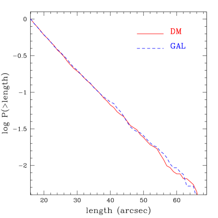
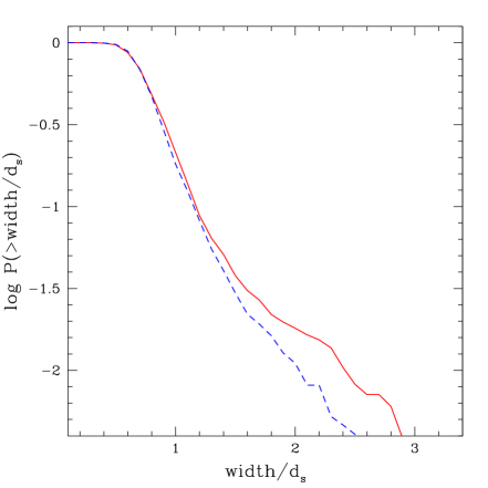
Figure 4: The cumulative distributions for the lengths $l$ (in units of arcsec) and the widths $w$ (in units of the source equivalent diameter $d_{\rm s}=2^{\prime\prime}$) are presented in the left and right panels, respectively. Results for the DM and GAL simulations are shown by solid and dashed lines, respectively. Typical bootstrap errors of the curves shown here grow from $\sim 5\%$ for small arcs to $\sim 15\%$ for large arcs.

The next step is the derivation of arc properties. We follow again the method proposed by Miralda-Escudé [1993] and Bartelmann & Weiss [1994]. We define the area of each image as the total number of image points. The circumference is defined as the number of boundary points, i.e. the number of image points which are not completely enclosed by other image points.

We then find a circle crossing three image points, namely (a) its centre, (b) the most distant boundary point from (a), and (c) the most distant boundary point from (b). Since we use a grid on the image plane, we cannot exactly find the centre of the image, and we have to choose the image point which is mapped next to it. Notice that long arcs can be merged from a few images, and there might exist more than one image of the source centre. However, this is not a problem because these points are located almost on the same circle.

We define the length $l$ and the curvature radius $r$ of the image through the circle segment within points (b) and (c). To determine the image width $w$, we search a simple geometrical figure with equal area and length. For this fitting procedure, we consider ellipses, circles, rectangles and rings. In the various cases, the image width is approximated by the minor axis of the ellipse, the radius of the circle, the smaller side of the rectangle, or the width of the ring, respectively. A possible test for the quality of the geometrical fit is given by the agreement between the circumferences of the geometrical figure and the image.

4.2 Results

4.2.1 General properties

For our statistical analysis we can use the results of 27 DM simulations and the same number of GAL simulations produced by the three projections along the Cartesian axes of nine clusters, which are quite different, both in masses and shapes. As can be seen from Fig. 2 of Tormen et al. [1997], some of the structures are more relaxed and show only one central density peak. In other cases the clusters have evident substructures, and they are still in a dynamical phase. Some of their lensing characteristics depend on these properties. Regardless of the presence or absence of cluster galaxies, the most massive clusters are the strongest lenses, as expected. For example, the number of giant arcs (hereafter defined as the arcs having a length larger than $16^{\prime\prime}$) produced by the g15 cluster (having a mass of $\simeq 3\times 10^{15}M_{\odot}$) is almost a factor 8 larger than the number of those produced by the less massive cluster of our sample (g40, with $M_{\rm vir}\simeq 5.3\times 10^{14}M_{\odot}$).

As already noticed by Bartelmann & Weiss [1994] and Bartelmann, Steinmetz & Weiss [1995], there is a strong influence on arc statistics due to asymmetries and substructures in the clusters. We find the same result in our sample (both in DM and GAL simulations). The median of the distribution of the widths of giant arcs is significatively smaller in the most compact projection with respect to the other ones (e.g. $w\simeq 2.6^{\prime\prime}$ versus $w\simeq 3.6^{\prime\prime}$ for cluster g81 and $w\simeq 3.2^{\prime\prime}$ versus $w\simeq 4.2^{\prime\prime}$ for cluster g40). On t he contrary, the median of the length-to-width ratios is smaller for the projections with a shallower density profile (e.g. $l/w\simeq 10$ versus $l/w\simeq 18$ for cluster g81 and $l/w\simeq 9.5$ versus $l/w\simeq 15$ for cluster g40). This means that there is a larger probability to have long and narrow arcs when the lens is more compact, i.e. when the central value of the convergence $\kappa$ is larger. Secondary overdensities can also affect arc statistics. In fact, they produce a shear field $\gamma$ which can change the shape of the critical lines, defined as the curves on which $\det A=(1-\kappa)^{2}-\gamma^{2}=0$. We find examples (e.g. the cluster g15) in which large values of $\gamma$ can move the tangential critical lines to regions where the convergence $\kappa$ is small.

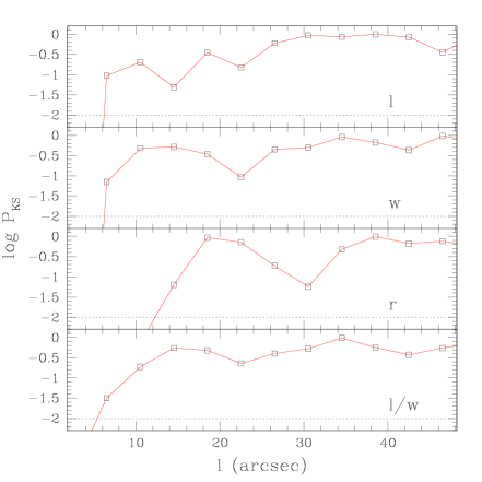
Figure 5: The behaviour of the probability $P_{\rm KS}$ (as computed in a Kolmogorov-Smirnov test) that the arc property distributions in data sets obtained from the simulations DM and GAL can be drawn from the same parent distribution. Subsamples of arcs with a given length $l\pm 2^{\prime\prime}$ are considered. The panels refer to different properties: length $l$, width $w$, curvature radius $r$ and length-to-width $l/w$ from top to bottom. The dotted lines show the 1 per-cent level.

4.2.2 Distributions of the arc properties

We now present the statistical analysis of the arc properties (length $l$, width $w$, length-to-width ratio $l/w$ and curvature radius $r$). We exclude from this statistical analysis all images represented by a single grid-point, i.e. produced by isolated rays: it would be impossible to define the previous quantities for them.

As mentioned previously, we assign to each arc a weight depending on the degree of the iteration in which the corresponding source was been placed. In practice, the weight is proportional to the sky area which is sampled by the source. The following distributions use this normalisation.

The total number of arcs in the whole set of DM and GAL simulations is quite similar: 447,112 and 451,782, respectively. The majority of these arcs is quite short. Considering only giant arcs, defined as arcs whose length is larger than $16^{\prime\prime}$, the sample reduces to 1,823 and 1,702 arcs for the DM and GAL simulations, respectively.

In Fig. 4, we show the cumulative functions of lengths and widths of these giant arcs. The length distributions (left panel) do not seem to be sensitive to the cluster galaxies. We found a similar result also for the distributions of arc curvature radii (not shown in the figure). On the other hand, the distributions of the arc widths (right panel) show some differences between DM and GAL simulations, in that the arcs are slightly thinner when galaxies are included. Consequently, some small differences are also found in the distributions of arc length-to-width ratios.

We checked by means of a bootstrapping analysis whether the distribution functions of arc properties are affected by the relative smallness of the cluster sample used. Across $10^{5}$ bootstrapped samples constructed from the source distributions behind our 27 cluster fields, the rms scatter about the mean reached at most $\sim 15\%$. Bearing in mind that there are order-of-magnitude differences between arc numbers expected in different cosmologies, such uncertainties in the arc cross sections are entirely negligible.

Therefore, the previous results seem to indicate that the characteristics of long arcs are only slightly changed by the presence of galaxies. In order to evaluate whether the differences between the two arc samples (DM vs. GAL) depend on the arc length, we selected subsamples of arcs with length in the range $l\pm\Delta l$ (with $\Delta l=2^{\prime\prime}$). Then, by performing a Kolmogorov-Smirnov test, we compare the arc property distributions in each subset of given arc length. We show in Fig. 5 the significance level obtained from the test as a function of $l$ for the four arc properties considered here: length $l$, width $w$, curvature radius $r$ and length-to-width ratio $l/w$. It can be seen from that plots that for all arc properties the probability $P_{\rm KS}$ that data sets obtained from the simulations DM and GAL can be drawn from the same parent distributions becomes lower than $1\%$ only for very short arcs. The differences are significant for $l\raisebox{-2.15277pt}{$\,\stackrel{{\scriptstyle<}}{{\scriptstyle\sim}}\,$}12^{\prime\prime}$ for the curvature radii, and for $l\raisebox{-2.15277pt}{$\,\stackrel{{\scriptstyle<}}{{\scriptstyle\sim}}\,$}4^{\prime\prime}$ for the other properties. Once again, these results indicate that giant arcs are generally not significantly perturbed by cluster galaxies.

Figure 6: Example of critical curves and arcs obtained in a DM (left panel) and GAL simulations (right panel). The angular dimensions of the plot correspond to $\simeq 333^{\prime\prime}$. It can be noticed that the presence of galaxies acting as gravitational lenses can split long arcs in several arclets, and increases the length of the critical curves.

5 Discussion and Conclusions

Three principal effects on the arc characteristics were expected due to the presence of cluster galaxies. First, the cluster critical curves wiggle around individual galaxies, increasing their length (see the example shown in the right panel of Figure 6). For this reason, the cluster cross section for strong lensing would tend to be increased and a larger number of long arcs would be expected.

At the same time, the curvature of the critical lines also increases. Galaxies could therefore perturb some arcs and split them into several shorter arclets, as can be seen for the longest arc in Fig. 6. Obviously, this effect acts such as to decrease the cross section for strong lensing.

Finally, the local steepening of the density profile near cluster galaxies tends to make arcs thinner.

The results of the Kolmogorov-Smirnov test indicate that the effect of cluster galaxies is negligible if very short arcs are excluded from the statistical analysis. This means than the first two effects previously mentioned are almost exactly counter-acting, and the splitting of some long arcs is compensated by the increased strong-lensing ability of the clusters.

Moreover, considering all the giant arcs (larger than $16^{\prime\prime}$), the galaxies tend to make them slightly thinner, as expected. However, this effect is weak, indicating that the galaxies do not produce perturbations strong enough to systematically affect all the arcs.

On the other hand, as confirmed by the Kolmogorov-Smirnov test, there are some significant differences between the property distributions of short arcs. These arcs do not form in the central regions of the clusters, where most of the mass is concentrated and where long arcs form instead. In such dense regions only a small fraction of the total galaxy mass emerges from the underlying dark-matter distribution. This does not happen in the outer regions of the clusters, where the dark matter density is lower and the galaxies stick out almost completely above the smooth cluster matter profile. For these reasons, the impact of such galaxies is stronger, and several secondary short critical lines form around them, as can be seen again in Fig. 6. Therefore, arcs forming far from the cluster centre tend to be shorter and thinner, with larger curvature radii, and the property distributions change significantly when the galaxies are included in the simulations.

Bootstrap resampling of the 27 cluster fields shows that the rms uncertainty of the cumulative arc distributions amounts to at most $\sim 15\%$, indicating that our cluster sample is large enough for the results to be reliable.

These results allow us to conclude that the granularity of the cluster potential due to the cluster galaxies has negligible effects on the statistics of giant arcs in an Einstein-de Sitter universe. What is more, we believe that we can conclude that cluster galaxies also have negligible effects on lensing by clusters in low-density universes. Such clusters form earlier and are therefore more compact than those in an Einstein-de Sitter universe. This implies that the strong-lensing cross sections contributed by individual cluster galaxies are relatively even less important compared to the cross sections of the clusters than in the Einstein-de Sitter case. If galaxies have no effect on arc cross sections under circumstances when the clusters themselves are the weakest lenses, they will be entirely negligible when embedded into stronger-lensing clusters. This also means that previous predictions of the number of large arcs produced by galaxy clusters via strong gravitational lensing, which were obtained from numerically modelled clusters in which individual galaxies are not resolved, can safely be used in comparisons with observational data.

Our results are well compatible with a recent independent study by Flores, Maller & Primack (1999), who perturbed a pseudo-elliptical cluster mass distribution with galaxies modelled as truncated isothermal spheres and found only a negligible enhancement of the smooth cluster’s arc cross section.

Appendix A Projected density profile of the galaxies

We present in this appendix the detailed formulae for the projection of the NFW density profile eq. (14) for the cluster galaxies.

Considering a galaxy with a truncation radius $r_{\rm t}$, the projected NFW density profile is given by

$$\Sigma_{{}_{\rm NFW}}(\xi)=2\int_{0}^{z_{\rm max}}\rho_{{}_{\rm NFW}}(r)\,{\rm d}z\ ,$$ (24)

where $z$ is the coordinate along the line of sight and $\xi$ is the component of $r$ perpendicular to $z$. The maximum of $z$ is given by $z_{\rm max}=\sqrt{r_{\rm t}^{2}-\xi^{2}}$.

Using the dimensionless coordinate on the projection plane $x\equiv\xi/r_{s}$ and defining the quantities $u\equiv\mbox{arcsinh}(z/\xi)$ and $\kappa_{\rm s}\equiv\delta_{\rm c}\rho_{\rm cr}\Sigma_{\rm cr}^{-1}$, the previous equation can be written as

$$\Sigma_{{}_{\rm NFW}}(x)=2\kappa_{\rm s}\Sigma_{\rm cr}f(x)\ ,$$ (25)

where

$$f(x) = -\frac{2}{(x^{2}-1)^{3/2}}\arctan\left[\frac{x-1}{\sqrt{x^{2}-1}}\tanh\left(\frac{u}{2}\right)\right]$$ (26)

$$+ \left.\frac{1}{x^{2}-1}\frac{x\sinh u}{1+x\cosh u}\right|_{0}^{u_{\rm max}}$$

if $x>1$;

$$f(x)=\frac{2\cosh(\frac{u}{2})\sinh(\frac{u}{2})}{3(1+\cosh u)^{2}}+\left.\frac{4\cosh(\frac{u}{2})^{3}\sinh(\frac{u}{2})}{3(1+\cosh u)^{2}}\right|_{0}^{u_{\rm max}}$$ (27)

if $x=1$; and

$$f(x) = \frac{2}{{1-x^{2}}^{3/2}}\mbox{arctanh}\left[\frac{1-x}{\sqrt{1-x^{2}}}\tanh\left(\frac{u}{2}\right)\right]$$ (28)

$$+ \left.\frac{1}{1-x^{2}}\frac{x\sinh u}{1+x\cosh u}\right|_{0}^{u_{\rm max}}$$

if $x<1$.

In the previous formulae, $u_{\rm max}=\mbox{arcsinh}(z_{\rm max}/\xi)$.

References

- [1993] Bartelmann M., Ehlers J., Schneider P., 1993, A&A, 280, 351
- [1998] Bartelmann M., Huss A., Colberg J.M., Jenkins A., Pearce F.R., 1998, A&A, 330, 1
- [1995] Bartelmann M., Steinmetz M., Weiss A., 1995, A&A, 297, 1
- [1994] Bartelmann M., Weiss A., 1994, A&A, 298, 1
- [1995] Bernstein G.M., Nichol R.C., Tyson J.A., Ulmer M.P., Wittman D., 1995, ApJ, 110, 1507
- [1995] De Propris R., Pritchet C.J., Harris W.E., Mc Clure R.D., 1995, ApJ, 450, 534
- [1999] Flores R.A., Maller A.H., Primack J.R., 1999, ApJ, submitted, preprint, astro-ph/9909397
- [1988] Hockney R.W., Eastwood J.W., 1988, Computer simulations using particles. Hilger, Bristol
- [1997] Lobo C., Biviano A., Durret F., Gerbal D., Le Fèvre O., Mazure A., Slezak E., 1997, A&A, 317, 385
- [1993] Miralda-Escudé J., 1993, ApJ, 403, 497
- [1996] Navarro J.F., Frenk C.S., White S.D.M., 1996, ApJ, 462, 563
- [1997] Navarro J.F., Frenk C.S., White S.D.M., 1997, ApJ, 490, 493
- [1993] Navarro J.F., White S.D.M., 1993, MNRAS, 265, 271
- [1999] Perlmutter S. et al., 1999, ApJ, 517, 565
- [ 1974] Press W.H., Schechter P., 1974, ApJ, 187, 425
- [1992] Richstone D.O., Loeb A., Turner E.L., 1992, ApJ, 393, 477
- [1997] Tormen G., Bouchet F.R., White S.D.M., 1997, MNRAS, 286, 865
- [1991] Van der Marel R.P., 1991, MNRAS, 273, 710
- [1998] Vedel H., Hartwick F., 1998, ApJ, 501, 509
- [1998] Wambsganss J., Cen R., Ostriker J.P., 1998, ApJ, 494, 29
- [1993] White S.D.M., Navarro J.F., Evrard A.E., Frenk C.S., 1993, Nat, 366, 429