Accretion flows: the role of the outer boundary condition
Abstract
We investigate the influences of the outer boundary conditions(OBCs) on the structure of an optically thin accretion flow. We find that OBC plays an important role in determining the topological structure and the profiles of the density and temperature of the solution, therefore it should be regarded as a new parameter in the accretion disk model.
keywords:
accretion, accretion disks – black hole physics – hydrodynamics1 Introduction
The behavior of an astrophysical accretion flow is described by a set of non-linear ordinary differential equations. Thus the outer boundary condition(OBC) possibly plays an important role in such an initial value problem. On the other hand, the complicated astrophysical environments make the states of the accreting gas at the outer boundary, such as its temperature and angular momentum, various. So it is necessary to investigate the role of OBC in accretion process.
However, this problem has not received enough attention until now. In the standard thin disk model the differential equations are reduced to a set of linear algebraic equations that don’t entail any boundary conditions at all. In the later works on the global solutions for slim disks the thin disk solution was usually adopted as the approximate OBC (Paczyński & Bisnovatyi-Kogan 1981; Muchoteb & Paczyński 1982; Matsumoto et al. 1984; Abramowicz et al. 1988; Chen & Taam 1993). In the case of optically thin accretion, this approach does not apply any longer because of the importance of the energy advection throughout the disk. In this case, self-similar solution by Narayan & Yi(1994), or some “arbitrarily” adopted value around the self-similar solution, is usually chosen as the OBC(Narayan, Kato & Honma 1997; Chen, Abramowicz & Lasota 1997; Nakamura et al. 1997; Manmoto, Mineshige & Kusunose 1997; Popham & Gammie 1998). They all concentrated on the solution under a specified boundary condition, while the role of OBC was not considered. Shapiro(1973) is an exception. In the context of spherically accretion, he found that the temperature distribution and the radiation luminosity of the disk depended sensitively on whether the interstellar medium was an H I or an H II region.
In this Letter, taking the optically thin accretion as an example, we investigate the effects of OBC on the structure of the accreting flow.
2 Equations and Results
We consider a steady axisymmetric accretion flow around a black hole of mass ( throughout this Letter), employing a set of height-integrated equations widely used by the present workers. Paczyński & Wiita (1980) potential is used to mimic the geometry of a Schwarzschild black hole. We first assume that the couple between the electrons and ions is so strong that the flow is a one temperature plasma. The equations read as follows:
| (1) |
| (2) |
| (3) |
| (4) |
All the quantities have their popular meanings. The shear stress is taken to be simply proportional to the pressure, i.e., shear stress=. We assume the flow is optically thin, so the pressure is dominated by gas pressure, . For simplicity the bremsstrahlung emission is assumed to be the only cooling process. The viscous heating and radiation cooling rates are
| (5) |
| (6) |
respectively.
Since the accretion onto a black hole must be transonic, the solution must satisfy the sonic point condition at a certain sonic radius . Besides this, we require the flow must satisfy two outer boundary conditions at a certain outer boundary . (Note that the no torque condition required at the black hole horizon is automatically satisfied under our viscosity description). As are given, we obtain the global solution by adjusting the eigenvalue to ensure that the flow satisfying the outer boundary condition satisfies the sonic point condition as well.
At , the two outer boundary conditions we imposed are and . This set of boundary conditions are equivalent to according to eq. (3) because is not a free parameter. We assign () to different sets of values and investigate their effects on the global solutions. The results are as follows.
As , and are given, we find that only when and are within a certain range do the global solutions exist. For example, for the global solutions with and (Here the Eddington accretion rate reads and is the Schwarzschild radius), the values of are close to the virial temperature (), . This range changes slightly when we modify the values of and , and when we consider different radiation mechanisms.
The solutions are remarkably different under different OBCs. In terms of the values of , the whole parameter space spanned by and can be divided into two regions. The solutions located in the low-temperature region(referred to as type I) have the following features, as the solid line in Fig. 1 shows: 1) the maximum feasible value of is close to 1; 2) a maximum exists in the solution’s angular momentum() profile; 3) the sonic radius is always small; and 4) the Bernoulli parameter , which is equivalent to is negative at large radii. The solutions located in the high-temperature region can be further divided into two types in terms of the values of . When is smaller than a critical value (referred to as type II), the sonic radii of the corresponding solutions are still small, but the values of become positive. Besides these, the angular momentum and the surface density() profiles and the topological structures(Mach number profile) differ greatly from those of type I, as shown by the dot-dashed line in Fig. 1. When is greater than (referred to as type III), suddenly becomes very large, as Table 1 and the dashed line in Fig. 1 show. This is a new kind of solution, since all previous works on ADAFs global solutions only obtained solutions with small values of . This kind of solution is difficult to be found because the parameter space where it is located is too narrow.
It is interesting to note that such transition of the values of is similar to that in the adiabatic case(Abramowicz & Zurek 1981). In that case, and are two constants of motion. When lies in a certain range, will jump from a small value to a large one when decreases across a critical value , and the corresponding accretion patterns are called disk-like(small , large ) and Bondi-like(large , small ) ones respectively. Our result indicates that such transition still exist although the flow becomes viscous(note that the increase of corresponds to the decrease of the angular momentum).
In general, modifying (i.e., modifying ) has much smaller effects on the solution than modifying does. The latter has a great effect on the topological structure and the profiles of the angular momentum and surface density of the solutions. But its effect on the temperature profile rapidly weakens with the decreasing radii, as the temperature profile plot in Fig. 1 shows. We’ll discuss this problem later.
The above calculation indicates that, besides and , OBC is also a crucial factor to determine the structure of the accretion flow.
Present theoretical and observational works seem to support the two temperature plasma assumption with the ions being much hotter than the electrons. In the following we consider whether the effects of OBC are still important in this case. Comptonization of the bremsstrahlung photon is also included in the cooling processes. The pressure and the energy equations should be replaced by,
| (7) |
| (8) |
| (9) |
where and denote the ion and electron molecular weights respectively, are the internal energies of the ion and electron per unit mass of the gas. Since for the temperature of interest, the ion is always unrelativistic while the electron is transrelativistic, following Shapiro(1973), we adopt the following:
| (10) |
in eq. (9) is the energy-transfer rate from the ions to electrons per unit volume duo to Coulomb collisions(Dermer, Liang & Canfield 1991):
| (11) |
where is the Coulomb logarithm, and is the dimensionless temperature. The thermal bremsstrahlung amplified by Comptonization reads( Rybicki & Lightman 1979) as follows:
| (12) |
| (13) |
| (14) |
Eqs. (7)-(14) together with eqs. (1)-(3) constitute the set of equations describing a two temperature accretion flow. In this case we must supply three physical quantities at , e.g. and . Obviously, for a given , the upper limit of is while its lower limit is determined by , i.e. all the energy transferred to the electrons is radiated away.
We solve the above set of equations under different OBCs and find that the results are qualitatively the same, as shown by Fig. 2. In this case we still find three types of solutions, the effect of is still unimportant for an individual type of solution, and the surface density profiles still differ greatly for the solutions with different OBCs. Compared with the corresponding solution in Fig. 1, the value of of the type I solution (denoted by the solid line in Fig. 2) decreases greatly. This is due to the inclusion of Comptonization together with the high surface density of the flow.
A remarkable new feature is that the electron temperature profiles of the solutions with different OBCs(primarily ) strongly differ from each other throughout the disk, while for the ion the discrepancies rapidly lessen with the decreasing radii from like a one temperature plasma. This is because the electrons are essentially adiabatic in the present low case, i.e., both and are very small compared with the two terms on the left hand side of eq. (9), so the electron temperature is globally determined therefore the effect of OBC on persists as the radius decreases. But for the ion, as well as the one temperature plasma, the local viscous dissipation in the energy equation plays an important role thus the energy equation for ions is much more “local” than that for electrons, so the effect of OBC weakens rapidly with the decreasing radii. Due to the same reason, we predict that OBC will be less important in determining the temperature profile of an optically thick accretion flow, since both the viscous dissipation and the radiation losses terms in the energy equation are important thus the temperature will be locally determined. But the flow should still present OBC-dependent dynamical behavior in , for example, the surface density and angular momenta profiles and the topological structure.
3 Conclusions
In this Letter, taking the optically thin one temperature and two temperature plasma as examples, we investigate the role of the outer boundary condition in the accretion process and find that it plays an important role. Our results indicate that in either case the whole solutions can be divided into three types in terms of their OBCs. The topological structures and the profiles of the angular momenta and the density are strongly different among the three types. As to the temperature we find that for a two temperature plasma the discrepancies of among the solutions with different OBCs will persist throughout the disk, while for ions and a one temperature plasma the discrepancies of the temperature rapidly lessen away from the outer boundary. Such discrepancies among the dynamic quantities will further induce the discrepancies of the radiation luminosity and the emission spectra of the accretion disc. Therefore we argue that OBC should be regarded as a new parameter in the accretion model.
Acknowledgements.
F.Y. thanks Dr. Kenji E. Nakamura for helpful discussions and the anonymous referee for useful suggestions to improve the presentation of this paper. This work is supported in part by the National Natural Science Foundation of China under grants 19873005 and 19873007.References
- (1) Abramowicz, M. A., Czerny, B., Lasota, J. P., & Szuszkiewicz, E., 1988, ApJ, 332, 646
- (2) Abramowicz, M., A., Zurek, W.H., 1981, ApJ, 246, 31
- (3) Chen, X., Abramowicz, M. A., & Lasota, J.-P. 1997, ApJ, 476, 61
- (4) Chen, X., & Taam, R.E. 1993, ApJ, 412, 254
- (5) Dermer, C.D., Liang, E.P., & Canfield, E. 1991, ApJ, 369, 410
- (6) Manmoto, T., Mineshige, S., Kusunose, M. 1997, ApJ, 489, 791
- (7) Matsumoto, R., Kato, S., Fukue, J., & Okazaki, A.T. 1984, PASJ, 36, 71
- (8) Muchotreb, B., & Paczyński, B. 1982, Acta Astron. 32, 1
- (9) Nakamura, K. E., Kusunose, M., Matsumoto, R., & Kato, S. 1997, PASJ, 49, 503
- (10) Narayan, R., Kato, S. & Honma, F. 1997, ApJ, 476, 49
- (11) Narayan, R. & Yi, I. 1994, ApJ, 428, L13
- (12) Paczyński,B., & Bisnovatyi-Kogan, G. 1981, Acta Astron., 31, 283
- (13) Paczyński, B., & Wiita, P. J. 1980, A&A, 88, 23
- (14) Popham, R., & Gammie, C.F. 1998, ApJ, 504, 419
- (15) Rybicki, G., & Lightman, A.P. 1979, Radiative Processes in Astrophysics (New York: Wiley)
- (16) Shapiro, S.L. 1973, ApJ, 180, 531
- (17)
- (18)
- (19)
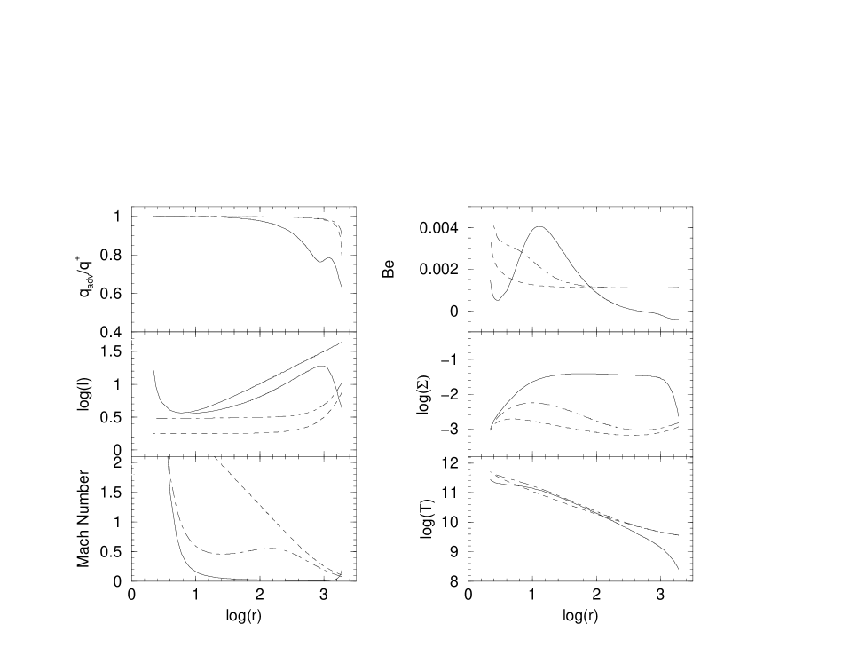
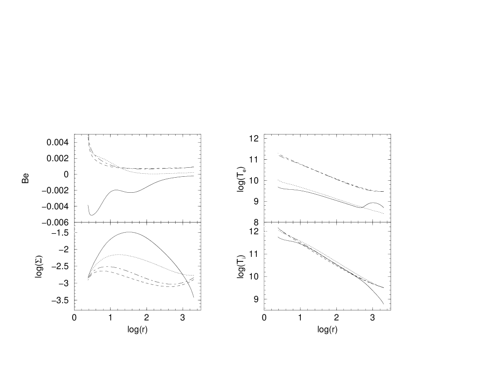
Table 1.
| (K) | ||||||
| 0.2 | 4.5476 | 3.4962 | ||||
| 0.4 | 4.5587 | 3.4887 | ||||
| 0.8 | 4.5531 | 3.4841 | ||||
| 0.08 | 5.7798 | 2.9869 | ||||
| 0.1 | 6.2359 | 2.8973 | ||||
| 0.102 | 155.1994 | 2.8023 | ||||
| 0.107 | 176.3544 | 1.7578 | ||||
| 0.3 | 7.0615 | 2.3171 | ||||
| 0.55 | 7.4851 | 2.2879 | ||||
| 0.556 | 701.0070 | 2.1473 | ||||
| 0.57 | 736.4865 | 1.2885 |