An Attempt to Pin Down the Instability Domain of Long-Period Variables

Abstract

The period-luminosity relation of Miras and semiregular variables in the Large Magellanic Cloud and in the Galaxy is used to locate their instability domain in the Hertzsprung-Russell diagram. We take advantage of the considerable width in luminosity of the relation at given period to assign masses to the observed long-period variables using stellar models on the the asymptotic giant branch and nonadiabatic pulsation computations. We study the sensitivity to chemical abundance of the position of the instability region on the Hertzsprung-Russell diagram. The mass function of the long-period variables along the AGB is discussed for Galactic and LMC variables. Finally, we contribute to the dispute on the pulsation mode of Miras and lend support to the view that, for most of the Mira variables, the pulsation in the fundamental mode is more likely.

1 Introduction

The first Mira variable was observed more than 400 years ago, nevertheless our astrophysical understanding of the Miras as a class is still far from satisfactory. The lack of understanding pervades stellar-evolution as well as pulsation aspects. Since these AGB stars are very cool and extended, their envelopes are dominated by convective energy transport and any successful theory explaining their variability needs to incorporate a trustworthy pulsation-convection interaction. To test the predictions of linear stability analyses which incorporate some sort of convection interaction formalism (e.g. Xiong et al. xdch98 (1998)), the results have to be compared with the observed boundaries of the Mira instability domain on the Hertzsprung-Russell (HR) diagram. Such an instability domain is missing in the literature, probably partly due to the complexity of assigning reliable temperatures to these large-amplitude variables at low temperature.

Besides Mira variables with large-amplitude and long-period pulsations, the AGB hosts – among others – also semiregular variables. The members of subclass a of the latter family (SRa) look very much like Miras, except for the smaller light-variability amplitudes. In the following, we will collectively refer to long-period variables (LPVs) when addressing Miras and SRas.

Astronomers agree on LPVs to be radial pulsators which oscillate mostly in one mode only. But already the assessment of the radial order of the pulsation mode in particular of Miras led to a long-lasting and ongoing controversy in the literature. The transformation of photometric color indices to temperatures is difficult at the low temperatures of the Miras and the adopted choice influences the derived pulsation mode. Interferometrically determined diameters and a low-temperature scale to assess surface temperatures favor first overtone modes (e.g. Tuthill et al. tutetal94 (1994), Haniff et al. hanetal95 (1995), Feast feast96 (1996), Barthès barth98 (1998) and references therein). On the other hand, based on period ratios between low- and high-amplitude long-period variables in the LMC, Wood & Sebo (ws96 (1996)) conclude that fundamental-mode pulsation is to be preferred for Miras. For a few years now, also theoretical studies favor Miras to pulsate in the fundamental mode (e.g. Ya’ari & Tuchman yt96 (1996), Tuchman t99 (1999)). Today’s numerical treatment of convection still hampers the reliability of these long-term simulations. But even along the linear-stability avenue, the lack of a trustworthy pulsation-convection interaction prescription prevented robust predictions. Only recently, Xiong et al. (xdch98 (1998)) reported non-adiabatic results with a sophisticated pulsation-convection interaction prescription. According to their results, the fundamental mode is clearly preferred.

The period-luminosity (PL) correlation of LPVs on the AGB is observationally well documented (e.g. Glass & Lloyd Evans gle81 (1981), Feast et al. fgwc89 (1989) and the references therein, Hughes & Wood hw90 (1990)). Currently, the true extension of the the PL correlation at fixed period seems to be an unsettled issue. Feast et al. (fgwc89 (1989)) presented a rather narrow relation whereas the Hughes & Wood (hw90 (1990)) data suggested a rather broad band. Various observational aspects – insecure periods, random-phase observations, biased data sets – can be responsible for the discrepancy. In any case, since LPVs are very luminous, they appear as attractive distance indicators. To exploit this potential, it appears seducing to find filter passbands or phases during the pulsation cycle which collapse whatever luminosity spread onto the narrowest possible band (e.g. Feast feast84 (1984), Hughes & Wood hw90 (1990), or Kanbur et al. khc97 (1997)). On the other hand, to study stellar physics, we are going to take advantage of the full spread of the PL relation and consider it as an additional source of information.

Since Mira variables are thermally pulsing AGB stars they follow the much referred to monotonous core-mass – luminosity relation only during a short fraction of a thermal-pulse cycle (cf. Wagenhuber & Tuchman wt96 (1996)). On first sight, a simple parameterization of the Miras’ position on the AGB appears to be no longer possible due to the non-monotonicity induced by the thermal pulses. On the PL plane, however, the situation improves considerably. During its numerous successive thermal pulses, an AGB star traces out a locus on the PL plane which almost collapses onto a single line. This line agrees very well with one traced out by a star which increases its luminosity monotonously as a function of core mass (see Fig. 3 of Wagenhuber & Tuchman wt96 (1996)). In other words, the locus traced out by an AGB star on the PL plane is a unique function of mass, independent of the phase during the thermal-pulse cycle. We take advantage of this property to assign masses to observed data and eventually map these data back onto the HR plane; this is the programme of the following paper. In section 2, we describe the observations which we utilized, the computational tools, and the assumptions entering the mapping of LMC and Galactic Mira data onto the HR plane. Section 3 contains the results which are discussed in Sect. 4. The latter section contains also the presentation of the mass functions derived for oxygen- and carbon-rich Miras in the LMC. The paper closes with some final comments (Sect. 5) on the consequences of our determination of the LPVs’ instability region.

2 Exploiting the PL relation

To infer the position of the instability domain of LPVs on the HR plane, we relied on luminosity estimates and period determinations for LMC and Galactic variables. The LMC data were collected from Hughes & Wood (hw90 (1990)), referred to as HW90. From Feast et al. (fgwc89 (1989)), abbreviated as FGWC89, we adopted a sample of LMC Mira variables. The latter brightness estimates are phase averaged. The HW90 magnitudes, on the other hand, were measured at random phase; as the number of objects in this sample is considerably larger, it is attractive to probe the extent of the instability domain. The HW90 data contain not only large-amplitude Miras but also SRa variables. Comparing the population of the PL plane by the two families of pulsators reveals no systematic difference. Therefore, we will not further distinguish between Miras and SRa’s but we will treat them equal and just refer to LPVs. It is worthwhile to stress that the two data sets, the HW90 and FGWC89 one, complement each other in the sense that the FGWC89 material tells something about the effect of random-phase observations (as in HW90) onto the PL relation. Despite the about 50% larger spread $\delta\!\log P$ at fixed $\log{L/L}_{\odot}$ of the HW90 data compared with the FGWC89 data set, we found no systematic shifts between the two populations on the PL plane. The origin of the considerably different $\delta\!\log P$ spread in HW90 and FGWC89 is an aspect which should be settled in the future as it influences the evolutionary interpretation of the LPVs.

Galactic PL data are very scarce and therefore extensive analyses are not possible to date. Nevertheless, in this paper we used the recently HIPPARCOS-calibrated Galactic Mira data published by van Leeuwen et al. (lfwy97 (1997)), referred to as vL97, and the results from Robertson & Feast (rf81 (1981)) (RF81).

To fit the observed PL data to theoretical data we performed pulsation modeling as described below. The stars’ loci along the AGB relied on their parameterization by Vassiliadis & Wood (vw93 (1993)):

$$\begin{split}\log{L/{L}_{\odot}}=-5\log{T}_{\rm eff}&+1.17\log{M/{M}_{\odot}}\\ &-0.581\log{Z/{Z}_{\odot}}+20.748.\end{split}$$ (1)

The set of masses on which the analyses are based comprise $0.8,1.0,1.5,2.0,3.0,4.0,$ and $5.0{M}_{\odot}$. For each mass, 20 models were computed according to eq. 1 in the range of $3.8<\log{T}_{\rm eff}<3.4$. Envelope integrations were carried out to a temperature of $10^{6}$ K. The surface boundary conditions were given by an atmosphere integration with a pseudo-spherical T-$\tau$ relation. Convection was treated in a non-adiabatic MLT fashion (Baker & Temeshvary bt66 (1966)) and turbulent pressure was accounted for in the momentum equation. The mixing-length was usually taken to be 1.5 pressure scale heights ($H_{\rm P}$). The influence of other choices are discussed in the text (Sect. 3). To set the magnitude of the isotropic turbulent pressure we chose $A_{\varpi}=1/3$ in our computations. The quantity $A_{\varpi}\equiv p_{\rm turb}/\rho w_{\rm c}^{2}$ measures the efficiency of generating turbulent pressure ($p_{\rm turb}$) out of the convection-induced Reynolds stress ($w_{\rm c}$ stands for the typical speed of the convecting eddies). Tests with different choices of $A_{\varpi}$ revealed no significant changes of the tracks on the $\Pi$L plane. In the following, we designate the theoretical period-luminosity results with $\Pi$L to distinguish them from observed PL data. Noticeable effect of adding turbulent pressure to the structure equations were observed only above about $\log L/{L}_{\odot}=3.75$. At fixed luminosity and for masses above $3{M}_{\odot}$, the periods of models computed with $A_{\varpi}=0.5$ were shifted up by at most about $0.07$ dex compared with model stars for which turbulent pressure was neglected. For lower-mass models the shifts were negligible (i.e. of the order of the thickness of the lines in Figs. 1 or 4).

Opacity tables were taken from the OPAL 1992 release (Iglesias et al. irw92 (1996)) which were extended with Alexander opacities at low temperatures (Alexander & Fergusson af94 (1994)). For the Galaxy we assumed $Z=0.02$ and $Z=0.01$ for the LMC.

Linear non-adiabatic (LNA) radial pulsation computations were performed with a Riccati-type code which derives from the version described in Gautschy & Glatzel (gg90 (1990)). For this study we considered fundamental (F) and first-overtone (O1) modes. The corresponding low eigenfrequencies still admit the use of reflective boundary conditions at the surface to be a decent approximation. This was inspected by computing the radial pulsation cavity in the adiabatic approximation. The eigenfrequency calculations neglected any pulsation-convection interaction. This crude approach is evidently inappropriate concerning imaginary parts of the eigenfrequencies. In other words, with this approach we can neither expect to determine the instability domain of Miras nor can we contribute anything to the solution of the pulsation-mode riddle. However, we are positive that the real parts of the eigenfrequencies, i.e. the periods, are sufficiently accurate for our purposes (cf. Xiong et al. xdch98 (1998)).

Figure 1: PL data of HW90 observations and results from radial pulsation computations. F-mode data for each mass choice is plotted as a solid line. The lowest line results from the $0.8{M}_{\odot}$ models. The masses $1.0,1.5,2.0,3.0,4.0,$ and $5.0{M}_{\odot}$ follow towards higher luminosities. The same ordering applies to O1 results displayed with dashed lines.

To derive the HR data and the mass function of the observed Miras on the PL plane we inverted the data from the previously described LNA analyses. To compute birational spline mass surfaces (Späth spaeth (1973)) on the $\Pi$L plane we needed the data on a regular rectangular grid. Therefore, we interpolated, with the piecewise-monotonic cubics algorithm of Steffen (steffen (1990)), periods and luminosities at appropriate positions along lines of constant mass. For the stiffness parameter of the birational spline we chose, after numerous experiments, always unity. The resulting mass, together with the observed period and an assumed abundance (based on the stellar system to which the LPV belongs) allowed the computation of an effective temperature according to the adopted AGB parameterization. Such an effective temperature has to be interpreted as the ‘equilibrium’ value and it can differ systematically from some phase-averaged mean effective temperature over an observed pulsation cycle. This aspect is further discussed in Sect. 4.

3 Results

First, we present the instability domains on the HR plane resulting from the inversion of observed pulsation data mapped onto the $\Pi$L plane. We start with the LMC and turn then to the modest Galactic data. In this section, we concentrate mainly on F-mode inversions to deduce the instability domain from the observations. If not noted otherwise, we used a mixing-length of $1.5H_{\rm P}$.

Figure 2: The inverted instability domain traced out by the HW90 data. The meaning of the symbols is the same as in Fig. 1. The solid lines indicate the loci of pseudo-evolutionary tracks on the HR plane based on eq. 1. The lowest mass gives the lowest line and they are ordered with increasing mass.

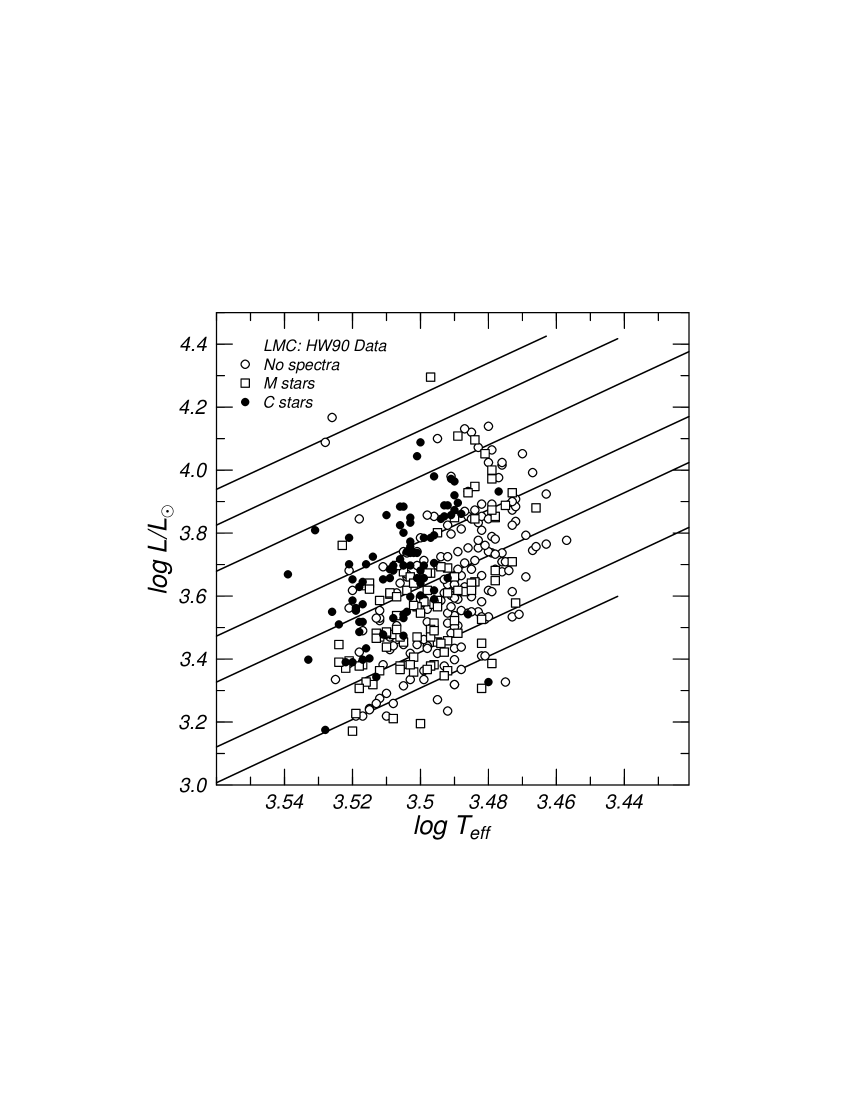
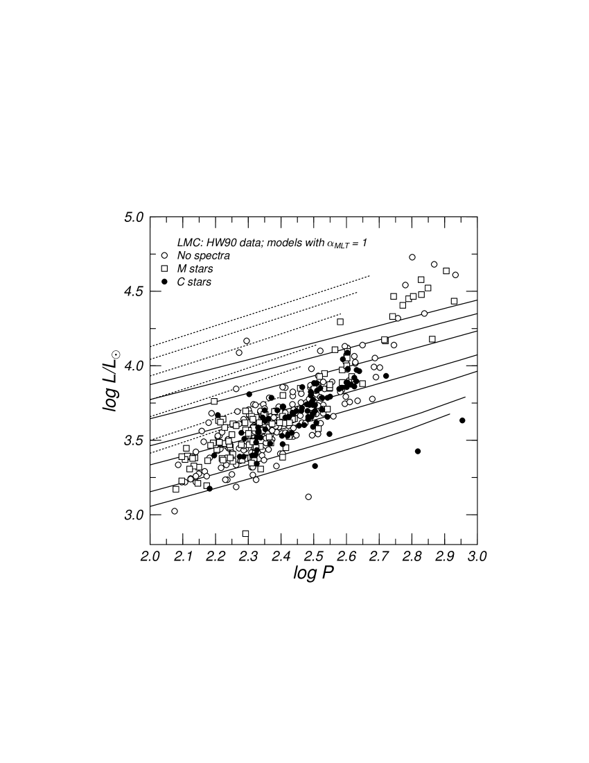
Figure 1 shows the PL (and $\Pi$L) diagram for the largest available data set, the HW90 data. Observations are plotted with open and filled symbols. The open ones represent either O-rich stars (also referred to as M-type stars in the figures) or stars for which no spectra (also abbreviated as NoSp stars) are available. C-rich variables are plotted with filled circles. Full lines show nonadiabatic radial F-mode periods as a function of luminosity for a fixed stellar mass and for an O-rich composition appropriate for $Z=0.01$. Dashed lines represent the same information but for the radial first-overtone (O1) mode. The various lines (of the same style) are ordered with respect to the mass of the stellar model. The lowest mass ($0.8{M}_{\odot}$) constitutes the lowest-luminosity line. For the inversion we restricted the period range to below about $500$ days and the luminosities to below $32\,000{L}_{\odot}$. At longer periods the simple-minded modeling of the stellar surface layers might no longer be justified by the large mass-loss rates observed. Within our restricted domain of inversion we could perform the analyses in the same fashion for the F as well as for the O1 modes.

Figure 3: Same as Fig. 2 but data was inverted with the assumption of O1 pulsations for all variables.

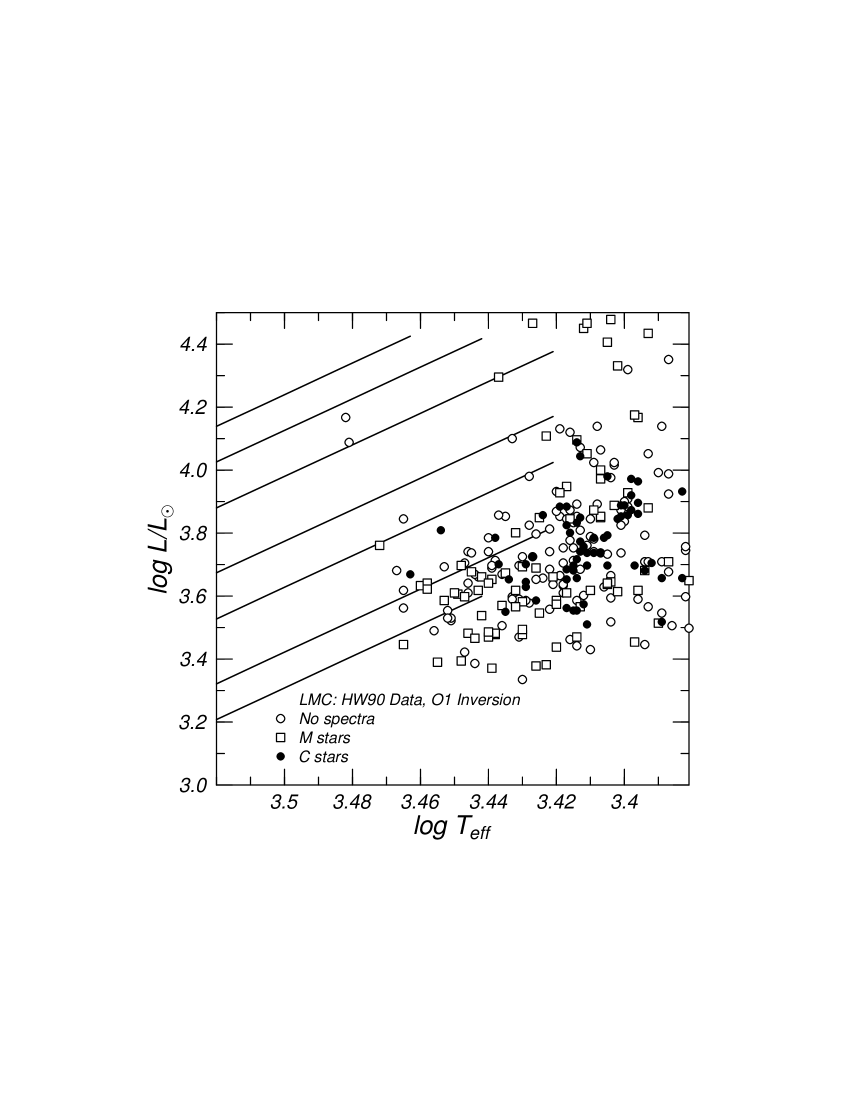
Figure 2 shows the inverted observational data projected onto the HR plane. We assumed all stars to pulsate in their F mode. For the O-rich variables and those without spectral information we used models with O-rich composition. The solid lines correspond to the tracks of different masses up the AGB, parameterized according to eq. 1. The masses are the same as those mentioned in the caption of Fig. 1. The lowest mass constitutes the lowest line and the order is monotonic. The C-rich stars were inverted with model stars which were computed with an abundance ratio (by number) C/O $=1.4$ but lying otherwise on the same tracks on the AGB as the O-rich stars. As cautioned by Hughes & Wood (hw90 (1990)), we found that the C-rich variables are attributed different masses and effective temperature than the O-rich ones when the different chemical compositions are incorporated in the model stars. This is particularly expressed in the F mode; inversions based on O1 modes are much less influenced by the composition choice. In case of the F mode, the $\Pi$L line is decremented by at most $0.05$ dex at fixed period at low masses and about half of that value above $4{M}_{\odot}$. If C-rich variables were analyzed with O-rich models, somewhat lower masses and lower effective temperatures were derived compared with an analysis referring to appropriate C-rich models.

The blue border of the instability domain is nearly vertical at $\log{T}_{\rm eff}\approx 3.53$. The red border, on the other hand, might be skew, broadening the instability domain towards higher luminosities. In any case, the red edge lies between $\log{T}_{\rm eff}=3.47$ and $3.45$. As we have no information on the completeness of the data sample we cannot estimate how robust the latter statement is.

Figure 4: Same as Fig. 1 but with the FGWC89 data.

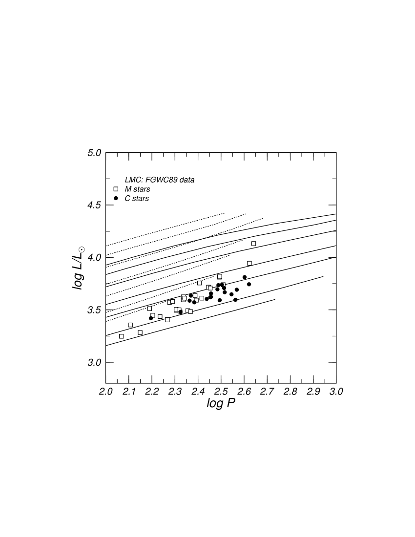
Figure 3 shows the results of the inversion of the the HW90 data assuming O1 modes only. The emerging instability domain has its blue boundary at $\log{T}_{\rm eff}\approx 3.47$. The boundary is not as clearly defined as in Fig. 2. A number of low-luminosity data points had to be removed as they were located too far from the lowest-mass $\Pi$L line so that the inversion failed. The red edge is located around $\log{T}_{\rm eff}=3.38$. Compared with Fig. 2, the data points are much more scattered at low temperatures in Fig. 3. Even if this visual impression alone is a weak argument against using the O1 assumption to find the instability domain, we will further substantiate the use of the F mode in Sects. 3.3 and 4.

The HW90 data are mostly based on single or few-epoch observations of the corresponding long-period variable stars. The large pulsation amplitudes of these variables might induce a vertical uncertainty in the distribution of Miras in the PL relation and a corresponding blurring of the true domain on the HR plane if only random-phase observations are used. Fortunately, we can check for such an effect in the HW90 data: Feast et al. (fgwc89 (1989)) published bolometric luminosities of a significantly smaller set of LMC Miras whose bolometric magnitudes were derived from averaging observations around the whole light-cycle. Figure 4 shows the corresponding PL data superposed on the same pulsation computations that were used for the HW90 data. Again, C-rich variables are plotted with a separate symbol (filled circles) to distinguish them from O-rich variables.

Figure 5: Same as Fig. 2 but with the FGWC89 data.

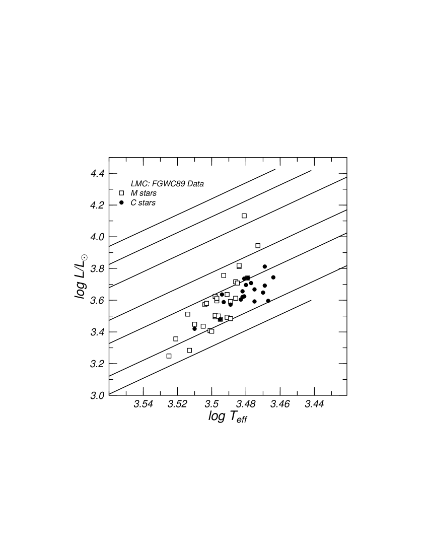
Figure 5 shows the sparsely populated HR domain after inversion of the FGWC89 data with the F-mode pulsation assumption. In contrast to HW90, the blue boundary – even if harder to define – appears to be cooler towards higher luminosities. A red edge is hard to define; in any case, no variables were found below $\log{T}_{\rm eff}\approx 3.46$. Despite the meager coverage of the PL domain we can observe that the FGWC89 data lie comfortably in the instability domain fenced by the HW90 data set. In other words, we do not see a systematic shift of the instability domains between the two LMC data sets. The blue edge of the FGWC89 instability domain is, however, clearly not vertical.

The analyses performed in the previous paragraphs are now applied to Galactic data. However, reliable measurements of absolute magnitudes are rare. In the following we discuss the Robertson & Feast (rf81 (1981)) and the recent HIPPARCOS-based measurements of $16$ galactic Miras published by van Leeuwen et al. (lfwy97 (1997)). With the available material we get at best a glimpse at the extent of the instability domain. At this stage, we infer again the instability domain from the assumption of F-mode pulsation only.

Despite the partial overlap only of the vL97 and the RF81 data-sets, we superpose them in Fig 7. This improves at least the appearance of the instability domain, even if its reliability does not.

Figure 6: Same as Fig. 1 for the Galactic data of RF81 and vL97.

Figure 7: Same as Fig. 2 but with the Galactic data of RF81 and vL97.

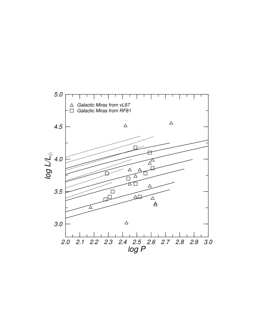
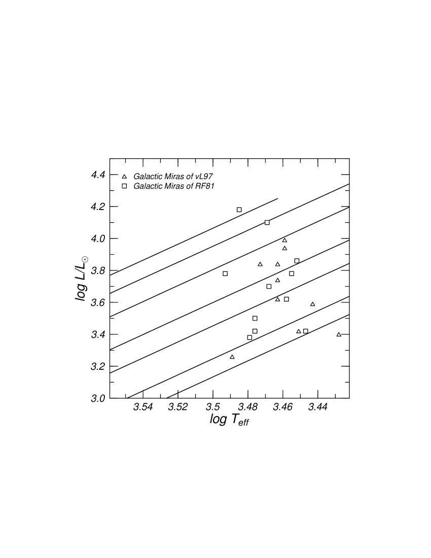
In spite of the low number of data points in each set we observe in Fig. 7 no systematic shift in ${T}_{\rm eff}$ between the two data sources. This is of course a direct consequence of compatible luminosity estimates – regardless of significant deviations of the magnitude estimates for some objects in common in both sets (cf. Fig. 6). The Galactic Mira data shown in Fig. 6 hint – again with the assumption of prevailing fundamental modes – at a blue boundary of the instability domain at $\log{T}_{\rm eff}\approx 3.49$. The red boundary is, once more, only ill defined; it is certainly as cool as $\log{T}_{\rm eff}=3.43$.

3.1 The effect of thermally modified stellar models

Recently, Ya’ari & Tuchman (yt96 (1996)) argued – based on long-term nonlinear model simulations – that Mira variables undergo mode switching from O1 to F mode as late as a few hundred years after the onset of the pulsational instability due to some nonlinear processes of the (thermo-)dynamical action of the pulsation on the thermal structure of the star. The mode switching is induced by the change of stellar structure which is also reflected in the change of the mean, as well as of the equilibrium radius of the star. Ya’ari & Tuchman conclude therefore that standard equilibrium stellar models, usually used to compute Mira pulsation properties are inadequate. In this subsection we investigate how strongly our inversion results change subject to a systematic shift of a variable star’s equilibrium radius.

According to the results published by Ya’ari & Tuchman (yt96 (1996)) the equilibrium radius of a model star lies close to the maximum compression phase of the dynamical pulsation. By comparing initial data with the state arrived at after about $500$ years we deduced that the equilibrium radius shrinked by about $29$%. We modeled such a shrinkage by modifying eq. (1) such that the tracks of a given mass on the HR plane were shifted to $29$% smaller radii. This procedure leads to the following relation:

$$\begin{split}\log{L/{L}_{\odot}}=-5\log{T}_{\rm eff}&+1.17\log{M/{M}_{\odot}}\\ &-0.581\log{Z/{Z}_{\odot}}+20.821.\end{split}$$ (2)

Compared with eq.(1), it is just the constant term which changes upon modifying the radius at a given luminosity. Models generated according to eq. (2) will be referred to as thermally modified (TM) hereafter.

Ya’ari & Tuchman’s (1996) result of pulsationally deflated radii founded on a modified entropy structure of the stars’ envelopes. Our models have, at a given luminosity, a smaller radius than what is predicted by canonical stellar evolution. Otherwise their envelopes are in thermal equilibrium. As we are interested in pulsation periods only, i.e. not in stability properties, we are confident that this crude approach is still a viable one.

Figure 8: Same as Fig. 1 but with thermally modified stellar models.

Computing the $\Pi$L relation for TM models revealed, comparing with canonical models, only minor shifts of the observationally well populated regions. The F-mode lines (solid lines in Fig. 8) are parallel-shifted to higher luminosities by at most $0.03$ dex at periods below about $300$ days. For longer periods the TM models show a steeper slope. For our inversion, this domain was not crucial as we restricted ourselves to LPVs with periods below $500$ days and the long-period population is rather small. As we see in Fig. 8, at fixed period the O1 lines are shifted vertically with respect to the fiducial lines shown in Fig. 1 by about $0.05$ dex for all masses and for the whole period range considered.

Mapping the HW90 data onto the HR plane using TM models revealed – in accordance with the statements in the last paragraph – that the locus of the instability domain which was computed by inverting F-mode $\Pi$L data was hardly affected. The blue border of the instability domain stayed at about $\log{T}_{\rm eff}=3.52$. Only the red border shifted to slightly lower effective temperatures, being now at around $\log{T}_{\rm eff}=3.45$.

We will further defend the inversion with the F-mode assumption in Sect. 4. Be it sufficient here to say that when using standard model stars in the analyses (as used in Sect. 3.1), the resulting preference of F modes for LPV pulsations there implies an even stronger preference of F modes in the case of using TM models. This applies in particular for the bulk of low-luminosity LPVs.

Notice that not only a deflation of a pulsating stellar envelope is encountered in nonlinear simulations: Dorfi (ead98 (1998)) presented preliminary results from radiation-hydrodynamical computations of a luminous blue variable model whose equilibrium radius increased by more than $10$% during the first few dozen pulsation cycles. The effect of an inflated equilibrium radius (compared with fiducial evolutionary tracks) is studied in the following subsection; the physical motivation to get there is a different one; the effect, however, is the same.

3.2 Changing the mixing-length

Tuchman (t99 (1999)) argued in his review that pulsation results of Miras, in particular the $\Pi$L relation, reacted sensitively on the choice of convection modeling – i.e. it reacts on the choice of the mixing length. We agree with that statement if we force the model star to remain at the same position on the HR plane during an MLT modification. However, it is not a priori obvious that the star’s position is not affected when its convection zones’ mixing length is modified. Therefore, we performed a set of stellar evolution computations with different mixing-length choices. Based on the resulting tracks we re-parameterized their AGB loci in accordance with the prescriptions used in eqs. (1) and (2). Tracks based on different mixing lengths for the convection zones were parallel-shifted relative to each other along the AGB. Models with larger mixing lengths ascended the AGB at higher effective temperatures. We arrived at a slope of $\Delta\log{T}_{\rm eff}/\Delta\alpha_{\rm MLT}=0.056$ in the range $1<\alpha_{\rm MLT}<2$. The results from the evolution computations and their transformation into the AGB parameterization led again to a change of the constant term in eq.(1). To study the influence of a low mixing length ($\alpha_{\rm MLT}=1$) on the $\Pi$L relation we used the following AGB prescription:

$$\begin{split}\log{L/{L}_{\odot}}=-5\log{T}_{\rm eff}&+1.17\log{M/{M}_{\odot}}\\ &-0.581\log{Z/{Z}_{\odot}}+20.72.\end{split}$$ (3)

Figure 9 shows that the LNA F-mode periods resulting from the $\alpha_{\rm MLT}=1$ AGB sequences are considerably longer at given luminosity and mass than what we deduced from, e.g., Fig. 1. This applied to all masses considered. The O1 periods, on the other hand, dropped slightly compared with the ‘fiducial’ choice of $\alpha_{\rm MLT}=1.5$ (and shown in Fig. 1). In other words, reducing the mixing length consistently, i.e. allowing also for modified evolutionary tracks, led to an enlarged period separation between F and O1 modes.

Figure 9: Same as Fig. 1 but with stellar models having a convection zones parameterized with $\alpha_{\rm MLT}=1$.

Hence, increasing the period at a chosen luminosity and fixed stellar mass favored again the interpretation of short-period LPVs as F-mode pulsators. On the $\Pi$L plane, the O1-period lines were shifted considerably upwards and led to very low masses (below $0.5{M}_{\odot}$) in the mass-fit of the inversion procedure. Therefore, we focus again on the F-mode results to estimate the location and shape of the instability domain. The considerable shift of the $\Pi$L lines in Fig. 9 of the F modes translated into a shift of the instability domain on the HR plane. The shift was purely horizontal since the luminosities are fixed observationally. We found the $\alpha_{\rm MLT}=1$ models to define an instability region which was shifted to higher temperatures by $0.025$ in $\log{T}_{\rm eff}$ when compared with the $\alpha_{\rm MLT}=1.5$ (cf. Fig. 2). The shape of the region remained unchanged.

3.3 The mass function of LPVs

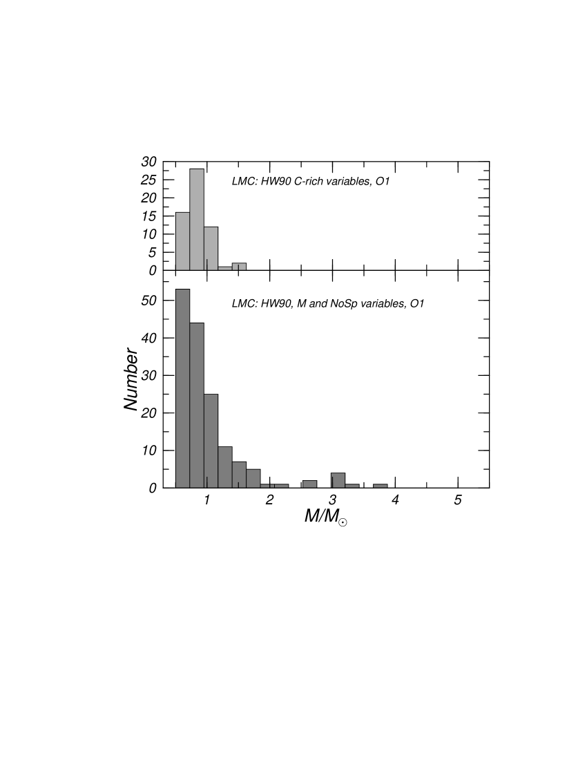
During the inversion procedure leading to the HR location of the data on the PL plane we assigned masses to the observed variable stars. Hence, we were in the position to derive a mass function of these variables along the AGB. As an example, we show the mass functions that were obtained during the inversion of the HW90 data, once with the assumption of F-mode pulsation (cf. Fig. 10) and once with the assumption of O1 pulsation (cf. Fig.11). The two figures are representative for all the the other data sets with which we worked. Independent of the choice of the observational data set, the shape of the distribution functions remained rather stable. The comparison of the HW90 data set with the FGWC89 one revealed that only the maxima of the distributions shifted slightly. This is rather surprising as we have to assume that the various observational data sets suffer from different selection effects. It is indeed only the change of the assumption on the pulsation mode which altered substantially the shape of the distribution function.

The figures showing the mass distributions are subdivided into C-rich stars and a plot collecting the rest of the sample, namely the O-rich ones and the variables lacking detailed spectral classification (NoSp).

For both inversions – assuming once F and then O1 modes – we explored the mass function in the range between $0.5$ and $5{M}_{\odot}$. For the F-mode pulsator assumption this domain embraces the resulting mass range well. For the O1 case, on the other hand, the number of low-mass pulsators increases rapidly and it continues so also below $0.5$ ${M}_{\odot}$. As the inversion becomes numerically problematic and physically questionable in this domain we ignored this range.

Figure 10: Mass function along the AGB derived for the HW90 data set with the assumption of F-mode pulsation only. The top panel shows the mass distribution for the C-rich stars in the sample. The bottom panel is made up of all other stars in the HW90 data (O-rich and stars without spectra). NoSp stands for no spectra available.

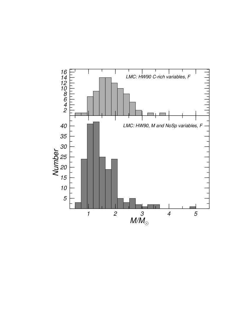
Figure 10 shows the well pronounced maxima of the mass function for the C-rich as well as in the non-C variables. The C-rich stars peak between $1.5$ and $1.8{M}_{\odot}$ whereas the maximum for non-C variables occurs at about $1.25{M}_{\odot}$. Both distribution functions show an asymmetric bell curve. The low-mass flank is steeper than the high-mass one in both cases. Up to slight shifts of the maxima, the results are surprisingly stable with respect to analyzing different data sets. The FGWC89 data show the maximum of non-C variables at $1.1{M}_{\odot}$ and the one of the C-rich ones at about $1.4{M}_{\odot}$.

When we performed the F-mode inversion with thermally modified envelopes the character of the mass functions remained unchanged; only the maxima shifted. Using the HW90 data on the TM models led to maxima at about $1.3{M}_{\odot}$ for the non-C and C-rich variables. Performing the analysis on $\alpha_{\rm MLT}=1$ models led to an upward shift of the maxima to $1.75{M}_{\odot}$ for both the C-rich and the non-C variables, without any other consequences for the distribution function.

For the Galactic data the mass functions are very uncertain due to the low number of stars in the samples. We obtained crude results only for the RF81 data, hinting at a mass-peak at about $1.25{M}_{\odot}$.

Figure 11: Same as Fig. 10 but with the assumption of O1 pulsations only.

Despite the surprising agreement between the mass functions of independently obtained data sets we must address their robustness with respect to possible biases. This can be done only for the HW90 data for which Hughes & Wood (hw90 (1990)) investigated this aspect. So we restrict our comments to this particular data set. Our mass function must be compared with their ‘raw distributions’ as a function of period. Having to contemplate the raw data is not further restrictive as it already reproduces the important aspects of showing a local maximum and the shape of the short-period and long-period flanks of the final distribution function which the authors (HW90) considered to be representative for the LMC. Assuming a unique relationship between ${M}_{\ast}$ and period would let us easily transform their ${\rm d}N/{\rm d}\log P$ plot (their Fig. 9) into our $N({M}_{\ast})$ plots (cf. Figs. 10 and 11). The Jacobian, ${\rm d}\log P/{\rm d}\log{M}_{\ast}$, is of order of unity and does not vary significantly over the period domain of interest so that the shape of the number of variables as a function of period is preserved along the mass coordinate. However, ${M}_{\ast}$ is not only a function of period alone but it depends also on luminosity. Therefore, the transformation is not that obvious and a preservation of the final form of the mass function cannot be expected a priori. Nevertheless, the number of long-period variable stars per mass interval seems to retain the shape found in ${\rm d}N/{\rm d}\log P$. The F-mode inversion is further supported by comparing our ${\rm d}N/{\rm d}{M}_{\ast}$ distribution with Iben’s (iben81 (1981)) ${\rm d}N/{\rm d}M_{\rm bol}$. The latter distribution shows also an asymmetric bell shape which is preserved when transformed into a mass scale. The Jacobian ${\rm d}M_{\rm bol}/{\rm d}{M}_{\ast}$ is of order unity and varies only slowly with stellar mass. Therefore, ${\rm d}N/{\rm d}M_{\rm bol}$ and ${\rm d}N/{\rm d}{M}_{\ast}$ are functionally roughly similar. If the aforementioned procedure is applied to the results of the O1 inversion, ${\rm d}N/{\rm d}M_{\rm bol}$ would remain a purely monotonously falling function towards brighter stars which does not agree with the Iben (iben81 (1981)) results.

4 Discussion

In the previous sections we demonstrated how the instability domain of LPVs can be deduced from period-luminosity data and linear non-adiabatic pulsation computations along an AGB parameterization which derives from stellar evolution calculations. With this approach we deduced effective temperatures which obtain for equilibrium models. We analyzed data of different sources for Galactic and LMC variables.

For the blue-edge position on the HR plane we claim to see a metallicity dependence. Reducing the heavy-element abundance shifts the blue edge to higher effective temperatures. The LMC blue edge is about $200$ K hotter than the one for Galactic Miras. The blueward shift of the blue edge of the instability domain upon lowering the heavy-element abundance is not attributable to the accompanying blueward shift of the evolutionary tracks alone. At the position of the blue boundary derived from LMC models we find evolutionary models with Galactic chemical composition. The latter have higher mass, however, and they do not yet pulsate. Only after further increase of their luminosity, i.e., lowered their mean density in the envelope, they start pulsating.

As an additional consistency test of our inversion we compared temperatures of Galactic Miras – computed with F-mode and with O1 assumption – as a function of period with data presented in Feast (feast96 (1996)). In this comparison we were interested in Galactic Miras with temperatures deduced by means of angular diameter measurements. These data present the ‘minimal’-assumption approach for our purpose. The Galactic F-mode pulsators’ temperature domain turned out to be compatible with about half of the observed variables, the rest of the observed stars was about $10$% cooler than what the inversion implied. When using the O1-assumption the situation reversed: About half of the stars with angular diameters had low enough effective temperatures to fit the inversion results and the rest turned to be roughly $10$% too hot.

We emphasize again that our effective temperatures correspond to equilibrium temperatures of the stars. These values can differ substantially from the pulsation-cycle averaged mean temperature. This point is emphasized in Fig. 12 where the nonlinear pulsation cycle of a $1{M}_{\odot}$ model star (model P7C14U4 of Höfner et al. hjla98 (1998)) is shown. From the vanishing time-derivative of the pulsational velocity we deduce the phases of passage through a quasi-equilibrium state. These phases are indicated with arrows in the bottom panel of Fig. 12. The corresponding ${T}_{\rm eff}$ values are rather close to the maximum of the ${T}_{\rm eff}$ curve. Therefore, as conjectured before, if simple averaging of temperature measurements over a pulsation cycle is done, we expect the resulting mean ${T}_{\rm eff}$ to be lower than the equilibrium values. In the model star shown in Fig. 12 the difference amounts to about $250$ K.

Figure 12: Model data of a radiation-hydrodynamic simulation of a pulsating $1{M}_{\odot}$ star at initially $7000{L}_{\odot}$. All physical variables at the photosphere are plotted over two periods which are folded onto the phase axis. The top panel shows the variation of the effective temperature. The middle panel displays the radius variation. The bottom panel contains the pulsational velocity of the photosphere. The two arrows in the bottom panel indicate the phases of passage through the equilibrium position of the model.

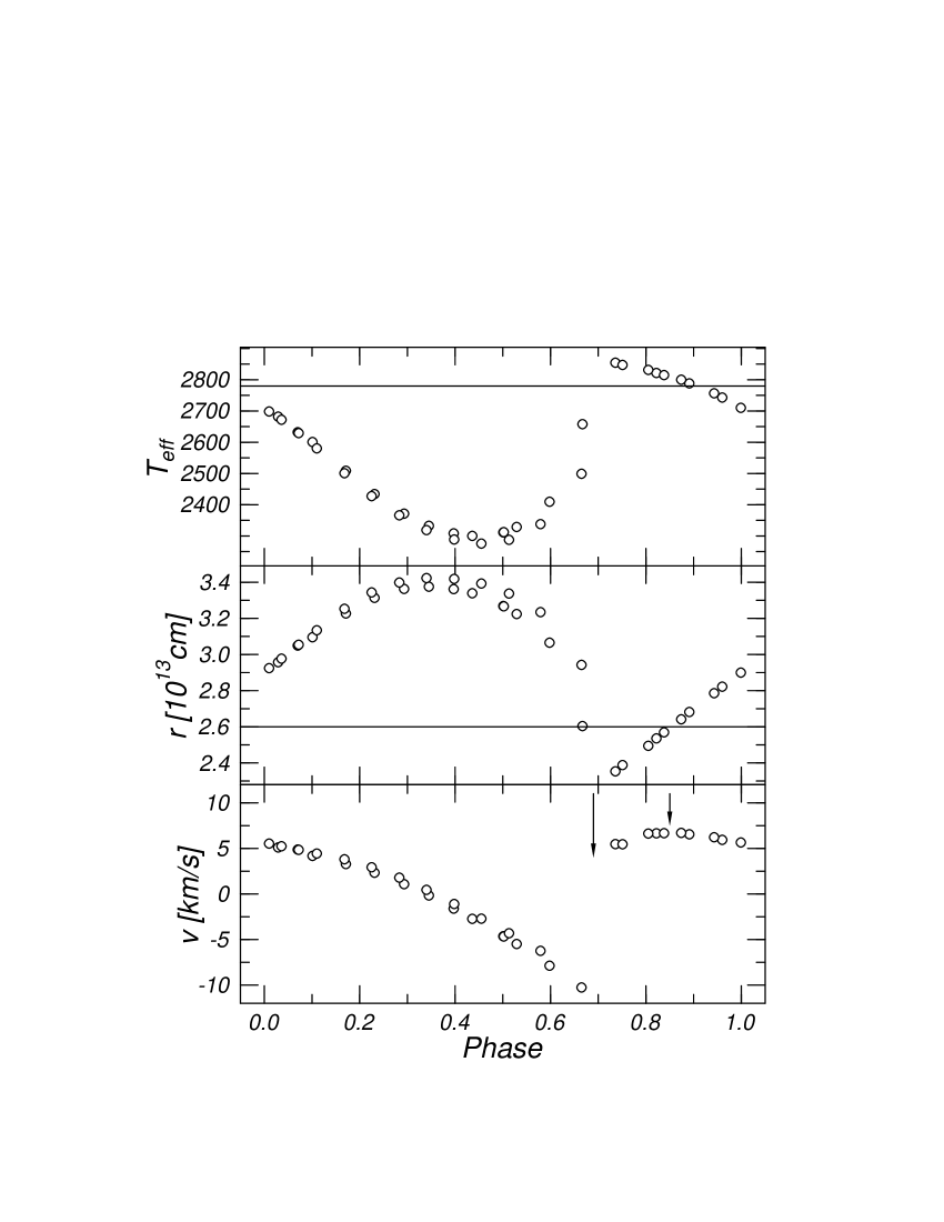
To finish the temperature discussion, we state our preference for the temperature scale which is derived from the F-mode data. The corresponding temperatures are slightly higher than what observations indicate. This, however, is in agreement with the discussion in the last paragraph. Notice that the slightly too high effective temperatures (compared with the equilibrium values) which are derived from observations are compatible with too large interferometrically determined radii measured at random phase. The middle panel of Fig. 12 shows that the equilibrium radius is close to the minimum radius and the mean – phase averaged – radius can exceed it by at least $10$%.

Along the process of deriving the instability domain we also computed masses for observational data points. Hence, we assigned masses to LPV stars and obtained mass functions for the different data sets. For a given assumption about the pulsation mode of the variables we found internally consistent functional forms of the mass functions for the different LMC as well as for Galactic data sets. In both stellar systems we arrived at a maximum of the mass functions at about $1.25{M}_{\odot}$ for the O-rich variables. The mass distribution of C-rich variables peaked between $1.5$ and $1.8{M}_{\odot}$. All the distributions resemble asymmetric bell-shaped functions with a steeper ascend on the low-mass side and a more gradual decline on the high-mass flank.

Carbon stars were treated separately in the inversion process to obtain their position on the HR plane. Accounting explicitly for this composition effect caused the observed C-rich variables to be assigned higher masses and higher effective temperatures than what we obtained when using O-rich models. The shift in mass, in particular below about $3{M}_{\odot}$, amounted to about $0.25{M}_{\odot}$. The effective temperature increased by about 0.025 in $\log{T}_{\rm eff}$. Treating the C-rich variables separately caused them to concentrate in the hot part of the instability domain. On the other hand, i.e. if treated the same way as the O-rich variables, the C-variables tend to lie in the cooler part of the instability domain. In either case, we found the C-variables to be slightly more massive than the O-rich LPVs. The functional forms of the mass function were comparable in both cases. Our approach of treating the C-variables with chemically appropriately modeled stars is only half way to the full solution as we still had to rely on the canonical AGB-track parameterizations such as in eq. (1) which is based on O-rich stars.

Figure 13: Variation of the pulsation constant as obtained from the nonadiabatic pulsation computations for LMC composition, $A_{\varpi}=0.5$, and $\alpha_{\rm MLT}=1.5$. Open circles represent F modes and filled ones the O1 results. The size of the circles reflect the stellar mass. This plot is representative for all other computations.

Figure 13 shows the variation of the pulsation constant $Q$ as a function of the pulsation period for F (open circles) as well as O1 (filled circles) modes of LMC models with $A_{\varpi}=0.5$ and $\alpha_{\rm MLT}=1.5$. The size of the symbols characterizes the model mass. The F-mode pulsations define a band with a width of about $0.02$ in $Q$ and it varies from roughly $0.05$ at $10$ days to $0.13$ at $1000$ days. The variation of the pulsation constant at fixed effective temperature as a function of mass (and hence luminosity) is traced out with the full line connecting the appropriate open circles. We observe that the paraboloid is more expressed the cooler the model stars are. In other words: In the low-luminosity range, the pulsation constant drops upon increasing the star’s mass. Once a critical luminosity (or mass) is reached, the pulsation constant rises again. This behavior is also reflected in the normalized oscillation eigenfrequency which shows a local maximum at the corresponding mass. We can understand the phenomenon as follows: At low masses, the mean-density decline upon increasing the stellar mass dominates over the associated period increase. At higher masses (and large enough luminosities) it is the pulsation-period lengthening with mass which over-compensates the mean-density reduction. The rather rapid increase of the pulsation period is attributable to the reduction of the mean adiabatic exponent $\Gamma_{1}$ across the pulsation cavity due to the growing contribution of radiation pressure which eventually forces the period to infinity as the limit of $\Gamma_{1}=4/3$ is approached.

The O1 results in Fig. 13, plotted with filled circles, show a much tighter correlation than the F-modes. The pulsation constant $Q$ varies only between $0.03$ and $0.04$ in the period range from $10$ to $300$ days. Additionally, the width in $Q$ at fixed period is very small. Functionally, however, the dependence of Q as function of stellar mass at fixed ${T}_{\rm eff}$ is the same as for F-modes. Only the amplitude of the variation is much smaller.

We conclude this section with a few elementary considerations of the expected width of the PL relation of pulsators on the AGB. Shibahashi (shib93 (1993)) argued that the convergence of the stars’ evolutionary tracks making up the AGB induce a mass dependence and therefore a substantial width into the PL relation. All the simple calculations can be done referring to eq. (1) and making use of the relation $\Pi\propto\sqrt{{R}_{\ast}^{3}/{M}_{\ast}}$. We begin by assuming a perfect coalescence of all evolutionary tracks on the AGB. In this case, any instability strip appears as a line on the HR plane and it is uniquely bordered by a lower and an upper luminosity. Even in this case, the $\Pi$L relation has a horizontal extension spanning $\delta\!\log\Pi=-0.5\cdot\delta\!\log{M}_{\ast}$ and vertical one extending over $\delta\!\log{L}_{\ast}=0.37\cdot\delta\!\log{M}_{\ast}$. The horizontal extent is purely a consequence of the pulsations being acoustic modes; the magnitude of the vertical width is influenced by the steepness of the evolutionary tracks which is taken from eq. (1). In this framework, we expect the PL data to form a rhombus with horizontal lower and upper border lines; the slope of the lateral border-lines (i.e. ${\rm d}\log{L}_{\ast}/{\rm d}\log\Pi$) is about 0.75. When we measure the horizontal spread in Figs. 1 and 4 we obtain a mass range $\delta\!{M}_{\ast}$ of about 0.8 (for HW90) and $0.55$ (for FGWC89) assuming a typical mass of $1{M}_{\odot}$ for these pulsating stars. These resulting mass ranges at constant luminosity appear unrealistically high so that we consider next a non-vanishing fan-out of the evolutionary tracks as a function of mass.

At constant luminosity, $\Pi$ is now more sensitive to the star’s mass than in the first case. We find $\delta\!\log\Pi=-1.16\cdot\delta\!\log{M}_{\ast}$. The mass range of variables at fixed luminosity reduces now to the more reasonable values of $0.35{M}_{\odot}$ for the HW90 and about $0.23{M}_{\odot}$ for the FGWC89 data. The $\log{L}_{\ast}({M}_{\ast})$ dependence remains essentially the same as in the coalescing-track scenario. In contrast to the simple first case, the shape of the instability domain influences now the shape of the $\Pi$L domain which is populated by LPVs. The narrower the instability strip is, the smaller the luminosity spread at fixed period. Furthermore, the larger the angle between the evolutionary tracks and the borderline of the instability domain on the $\Pi$L plane, the stronger the tendency for a large luminosity spread at fixed period even for a narrow instability strip. Since the evolutionary tracks and the very pulsational instability react on chemical composition, it is not further surprising that noticeable differences of PL relations in different stellar systems are reported in the literature (e.g. Menzies & Whitelock mw85 (1985), Feast et al. fgwc89 (1989)). Adding up the above aspects of widening the $\Pi$L relation of LPVs, the observation of a tight PL relation would be rather surprising.

5 Conclusions

We exploited the observed PL data by inverting them with the help of theoretical $\Pi$L results and derived the instability domain on the HR plane of LPVs in the LMC and of Miras in the Galaxy.

When inverting the PL data, model assumptions appeared to be not as crucial as advocated in the past: In particular, we found no significant effect of changing the mean radius of the model stars which is expected to happen when they experience finite amplitude pulsations (Ya’ari & Tuchman yt96 (1996)). Furthermore, the choice of the mixing length of convective eddies does not play an decisive rôle – if it is applied consistently to evolutionary models. As expected, however, the choice of the pulsation mode shifts the instability domain on the HR plane. Assuming O1-modes to be excited leads to an instability domain that is about $250$ K cooler than the instability domain inferred from F-mode pulsations. The blue edge of the latter instability region was found at about $\log{T}_{\rm eff}=3.52$ for LMC abundances. Finally, also the choice of the chemical composition is crucial. Treating the C-rich variables separately from the O-rich ones, turned out to be necessary. The position of the C-rich pulsators shifted from the cool side in the instability domain to the hot one when we performed the PL inversion with LNA results distinguishing between C-rich and O-rich objects. The shape and the location of the maximum of the mass function were, however, not influenced significantly.

As predicted by pulsation analyses including pulsation-convection interaction (Xiong et al. xdch98 (1998)) we encountered a shift of the instability domain to higher effective temperatures upon reducing the heavy-element abundances. In contrast to Xiong et al. (xdch98 (1998)), we clearly locate a blue edge of the fundamental mode.

The mass function which we obtained as a side-result peaks at about $1.3{M}_{\odot}$ for non-C variables and somewhere between $1.5$ and $1.8{M}_{\odot}$ for C-rich variables if we imply F-mode pulsation. This result is rather plausible. However, the numbers should be taken with care. The mixed-mode interpretation mentioned in the last paragraph and/or changing the chemical abundances will shift the maxima. In particular, lowering the heavy-element abundances reduces the mass at maximum. Nevertheless, the shape of the distribution function might be preserved. In case of a mixture of pulsation modes throughout the instability domain, we find O1 modes to be more likely (regarding the inferred mass) in the upper luminosity range.

The assumption that the mass function can be translated into a luminosity function and the comparison of the result with the literature led us to favor a fundamental-mode dominated explanation of LPV pulsations. A comparison of the predictions of Iben (iben81 (1981)) with our results showed at least a structural agreement of the F-mode mass function with the luminosity functions expected from stellar evolution. Assuming a O1 dominated mass-function with its exponential increase to lower masses appears unlikely according to this exercise.

For Miras and SRas, the evolutionary scenario bringing them into their instability domain remains obscure. If the hypothesis that the LPVs evolve in ${L}_{\ast}$ and $P$ during their overstable phase applies depends on the choice of the data set; the HW90 data (see Fig. 2) would support it to some extend. In the FGWC89 this is much less pronounced, however. In any case, for both data sets, the instability domain is too extended in ${T}_{\rm eff}$ and $P$, when measured along evolutionary paths, to justify the postulation of a mass-dependent period at which the LPVs pulsate – without luminosity evolution – before they leave the instability domain. Despite the incompatibility with the Galactic and the LMC number density of planetary nebulae (e.g. Wood w90 (1990)), but probably in better agreement with the Miras’ long-lifetime suggestion by Whitelock & Feast (wf93 (1993)), it appears necessary that Mira variables, or LPVs in general, live through several thermal pulses. Otherwise, it is unclear how they can populate the cool part of the instability domain.

The mass dependence in the LPVs’ PL relation can be traced back to the acute angle of the stars’ evolutionary tracks along the AGB at which they enter the instability domain and the mutual convergence of the tracks along the AGB. For a star’s pulsation it is its total mass which is relevant; at the AGB the mass cannot be parameterized as a function of luminosity due to the near convergence of the evolutionary tracks and therefore it cannot be replaced in the period – mean-density relation. The radius appearing in the latter equation can be substituted by a luminosity parameterization of a characteristic locus in the instability domain (such as e.g. the blue edge or a ridge line). Eventually, we arrive at a $P({M}_{\ast},{L}_{\ast})$ relation (cf. Shibahashi shib93 (1993)).