Rossby Wave Instability of Thin Accretion Disks – II. Detailed Linear Theory

Abstract

In earlier work we identified a global, non-axisymmetric instability associated with the presence of an extreme in the radial profile of the key function ${\cal L}(r)\equiv(\Sigma\Omega/\kappa^{2})S^{2/\Gamma}$ in a thin, inviscid, nonmagnetized accretion disk. Here, $\Sigma(r)$ is the surface mass density of the disk, $\Omega(r)$ the angular rotation rate, $S(r)$ the specific entropy, $\Gamma$ the adiabatic index, and $\kappa(r)$ the radial epicyclic frequency. The dispersion relation of the instability was shown to be similar to that of Rossby waves in planetary atmospheres. In this paper, we present the detailed linear theory of this Rossby wave instability and show that it exists for a wider range of conditions, specifically, for the case where there is a “jump” over some range of $r$ in $\Sigma(r)$ or in the pressure $P(r)$. We elucidate the physical mechanism of this instability and its dependence on various parameters, including the magnitude of the “bump” or “jump,” the azimuthal mode number, and the sound speed in the disk. We find large parameter range where the disk is stable to axisymmetric perturbations, but unstable to the non-axisymmetric Rossby waves. We find that growth rates of the Rossby wave instability can be high, $\sim 0.2\Omega_{\rm K}$ for relative small “jumps” or “bumps”. We discuss possible conditions which can lead to this instability and the consequences of the instability.

Draft version

Subject headings: Accretion Disks — Hydrodynamics — Instabilities — Waves

1 Introduction

The central problem of accretion disk theory is understanding the mechanism of angular momentum transport. The angular momentum must flow outward in order that matter accrete onto the central gravitating object. Earlier work suggested hydrodynamic turbulence as the mechanism of enhanced turbulent viscosity $\nu_{t}=\alpha c_{s}h$, with $\alpha\leq 1$ a dimensionless constant, $c_{s}$ the sound speed, and $h$ the half-thickness of the disk (Shakura & Sunyaev 1973). However, the physical origin and level of the turbulence is not established (see [Papaloizou & Lin 1995] for a review). Recently, the magneto-rotational instability ([Velikhov 1959]; [Chandrasekhar 1960]; see review by [Balbus & Hawley 1998]) has been studied in $2D$ and $3D$ MHD simulations and shown to give a Maxwell stress sufficient to give significant outward transport of angular momentum ([Balbus & Hawley 1998]); that is, a statistically averaged, effective Shakura-Sunyaev alpha parameter is found to be $\alpha\sim 0.01$ (Brandenburg et al. 1995). However, significant questions remain. The simulation studies are local in that a shearing patch or box of the actual disk of size $\ll r$ is treated; and the boundary conditions on the top of the box have so far been unphysical. Furthermore, disks in some systems (e.g., protostellar systems) are predicted to have very small conductivity so that coupling between matter and magnetic field is negligible.

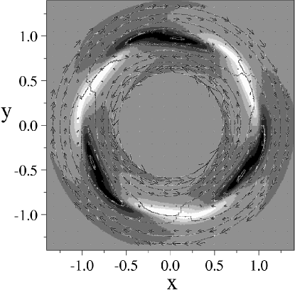
  Fig. 1.—: Illustration of the nature of the Rossby wave instability for $m=3$ for the case of a homentropic Gaussian bump centered at a radius $r_{0}=1$. The gray-scale component of the figure represents the surface density perturbation $\delta\Sigma$ with the darkest region the highest density. The contour lines and the arrows show the velocity field as seen in a reference frame rotating at the angular rate of the disk $\Omega(r_{0})$. This velocity field is $\Delta{\bf v}=\delta{\bf v}+\hat{{\hbox{\tenbg\char 30\relax}}~{}}[r\Omega(r)-r_{0}\Omega(r_{0})]$, where $\delta{\bf v}$ is the usual Eulerian velocity perturbation. The figure shows that the perturbation of the disk involves three anticyclones of closed streamlines or “islands” which approximately coincide with the regions of enhanced densities $\delta\Sigma$. The radial width of the “islands” has been exaggerated to make them visible.

Interesting fundamental questions still exist concerning pure hydrodynamic processes in accretion disks. One well-known hydrodynamic instability of disks is the Papaloizou-Pringle instability ([Papaloizou & Pringle 1984]; [Papaloizou & Pringle 1985]; hereafter PP) which has been extensively studied both in linear theory and by numerical simulations ([Blaes 1985]; [Drury 1985]; [Frank & Robertson 1988]; [Glatzel 1988]; [Goldreich, Goodman, & Narayan 1986]; [Kato 1987]; [Narayan, Goldreich, & Goodman 1987]; [Kojima et al. 1989]; [Hawley 1991]; [Zurek & Benz 1986]; see review by [Narayan & Goodman 1989]). In these studies, the “disk” is taken to be a thin torus (finite height) or annulus (infinite along $z$) with the radial width much less than the radius. The corotation radius, where the phase velocity of the wave $\omega_{r}/m$ equals the angular velocity of the matter $\Omega(r)$, has a crucial role in that a wave propagating radially across it can be amplified. However, significant growth of a wave typically requires many passages through the corotation radius and this requires reflecting inner and/or outer boundaries of the disk. Thus the PP instability depends on inner and outer disk boundary conditions which are artificial for accretion disks.

Recently, we pointed out a new Rossby wave instability of non-magnetized accretion disks ([Lovelace et al. 1999]; hereafter Paper I). Paper I shows that the local WKB dispersion relation for the unstable modes is closely analogous to that for Rossby waves in planetary atmospheres. Rossby vortices associated with the waves are well known in planetary atmospheres and give rise for example to the Giant Red Spot on Jupiter (Sommeria, Meyers, & Swinney 1988; Marcus 1989, 1990).

In the cases considered in Paper I, the instability occurs when there is a “bump” in the radial variation of ${\cal L}(r)\equiv(\Sigma\Omega/\kappa^{2})S^{2/\Gamma}$, where $\Sigma(r)$ is the surface mass density of the disk, $\Omega(r)$ the angular rotation rate, $S(r)$ the specific entropy, $\Gamma$ the adiabatic index, and $\kappa(r)$ the radial epicyclic frequency. Such a bump may arise from the nearly inviscid accretion of matter with finite specific angular momentum $\ell$ onto a compact star or black hole. The accreting matter tends to “pile up” at the centrifugal radius $r_{c}=\ell^{2}/(GM)$ (with $M$ the mass of the central object) where it gives a radially localized bump in ${\cal L}(r)$.

In accretion disks in some systems, such as active galactic nuclei, the weak self-gravity at large distances can be important in forming narrow rings (Shlosman, Begelman, & Frank 1990). Such rings would give a bump in ${\cal L}(r)$ of the form we have assumed. The bump in ${\cal L}(r)$ is crucial because it leads to trapping of the wave modes in a finite range of radii encompassing the corotation radius. Thus, reflecting inner and outer disk radii required for the PP instability are not required for the Rossby wave instability. In contrast with studies of the PP instability, we allow a general equation of state where the entropy of the disk matter can vary with radius.

The present paper develops in greater detail the work of Paper I and presents the full linear theory analysis of the instability without some simplifying assumptions made there. The physical nature of the Rossby wave instability is shown in Figure 1 where we have overlaid the velocity field onto the surface density variations. The basic theory is given in §2 and §3, and results are given in §4. In §5 we discuss the details of this instability and compare it with other hydrodynamic instabilities. Conclusions of this work are summarized in §6.

  Fig. 2.—: Parameters of the initial equilibrium for the homentropic step jump case (‘HSJ’): The pressure $P(r)/P_{0}$; the corresponding angular velocity $\Omega(r)/\Omega_{K}$; the square of the epicyclic frequency $\kappa^{2}(r)/\Omega_{K}^{2}$; and the effective sound speed $c_{s}/v_{K}$. The pressure jump is derived from a jump in surface density $\Sigma(r)$ with an amplitude ${\cal A}=0.65$ over $\Delta r/r_{0}=0.05$. This results in a pressure jump $(1+{\cal A})^{\Gamma}\approx 2.3$ for $\Gamma=5/3$. The disk rotation is close to Keplerian except near the region of the pressure jump. Note that $\kappa^{2}$ is everywhere positive.

2 Equilibrium Disks

We consider the stability of non-magnetized accretion disks. The disks are assumed geometrically thin with vertical half-thickness $h\ll r$, where $r$ is the radial distance. We use an inertial cylindrical $(r,\phi,z)$ coordinate system. The surface mass density and vertically integrated pressure are:

$$\Sigma(r)=\int_{-h}^{h}dz~{}\rho(r,z)~{},\quad\quad P(r)=\int_{-h}^{h}dz~{}p(r,z)~{}.$$

The equilibrium disk is stationary ($\partial/\partial t=0$) and axisymmetric ($\partial/\partial\phi=0$), with the flow velocity ${\bf v}\approx v_{\phi}(r)\hat{\phi}$; that is, the accretion velocity $v_{r}$ is assumed negligible. Self-gravity of the disk is assumed negligible so that $\Phi(r)=-GM/(r^{2}+z^{2})^{1/2}$, where $M$ is the mass of the central object. But we will discuss the effects of self-gravity in §5.

For the axisymmetric equilibrium disk, the radial force balance is:

$$\frac{v_{\phi}^{2}}{r}\equiv r\Omega^{2}=\frac{1}{\Sigma}\frac{dP}{dr}+\frac{d\Phi}{dr}~{}~{},$$ (1)

The vertical hydrostatic equilibrium gives $h(r)\approx(c_{s}/v_{\phi})r$, where

$$c_{s}^{2}\equiv\Gamma\frac{P}{\Sigma}$$ (2)

the square of adiabatic sound speed and $\Gamma$ is an effective adiabatic index discussed further in §3.

The focus of this paper is on the stability of equilibrium disks with a slowly varying background shear flow and a finite-amplitude density variation over a finite radial extent. Specifically, we envision conditions where inflowing matter accumulates at some radius, for example, a centrifugal barrier. This accumulation may occur if matter is supplied at a rate exceeding the rate at which matter spreads by say a turbulent viscosity. Depending on the angular momentum distribution of the incoming flow, newly supplied matter can form a disk with a finite “bump” or “jump” in the surface density at say $r$ with a radial width $\Delta r$. When the disk surface density is sufficiently small, the disk optical depth is small compared with unity and cooling by radiation is efficient. As more matter is accumulated, the disk becomes optically thick so that heat builds up inside the disk and can be vertically confined, then pressure forces start to have an important role for the disk dynamics. The present work is directed at optically thick disks with significant pressure forces.

We model the mentioned “bumps” and “jumps” with fairly general radial profiles of $\Sigma(r)$ and $P(r)$. These profiles are used to obtain the corresponding $\Omega(r)$ profile using equation (1). Specifically, we consider two surface density distributions: One is has a “step jump” from $\Sigma_{1}$ to $\Sigma_{2}~{}>~{}\Sigma_{1}$ over $\Delta r$ and this jump is surrounded by a smooth background flow,

$${\Sigma\over\Sigma_{\ast}}=1+\frac{\cal A}{2}\left[\tanh\left(\frac{r-r_{0}}{\Delta r}\right)+1\right]~{}~{},$$ (3)

where $\Sigma_{\ast}=\Sigma_{0}(r/r_{0})^{-\beta}$ is the surface density for the background disk, $\Sigma_{0}$ is its value at $r_{0}$ and $\beta$ characterizes the slope (it is $-3/4$ in a standard $\alpha$ disk model). Quantities ${\cal A}$ and $\Delta r$ measure the amplitude and width of the jump respectively, and $r_{0}$ is radius of the jump. The second case we consider is a “Gaussian bump,”

$${\Sigma\over\Sigma_{\ast}}=1+({\cal A}-1)\exp\left[-{1\over 2}\left(\frac{r-r_{0}}{\Delta r}\right)^{2}\right]~{},$$ (4)

where again, ${\cal A}$ and $\Delta r$ measure the height and width of the bump, respectively.

We assume an ideal gas equation of state, $P\propto\Sigma T$. Depending on whether the flow is homentropic or not, we can further derive or specify the radial distributions of temperature $T(r)/T_{0}$ and pressure $P(r)/P_{0}$ based on $\Sigma(r)$, where $T_{0}$ and $P_{0}$ are the values at $r_{0}$ for the background disk. We also set $v_{0}\equiv r_{0}\Omega_{0}$ to be the Keplerian speed at $r_{0}$, and define the dimensionless sound speed as $c_{0}^{2}\equiv\Gamma(P_{0}/\Sigma_{0})/v_{0}^{2}$. In most of the following analysis, we take $r_{0}=1$, $\Delta r/r_{0}=0.05$, $\Gamma=5/3$, and $c_{0}/v_{0}=0.1$.

  Fig. 3.—: Similar to Figure 2 but for the case of an homentropic Gaussian bump (‘HGB’). The peak of the surface density is ${\cal A}=1.25$ at $r=r_{0}$, which gives a peak of the pressure ${\cal A}^{\Gamma}\approx 1.45$ for $\Gamma=5/3$. Again, $\kappa^{2}$ is everywhere positive.

  Fig. 4.—: Similar to Figure 2 but for the case of a nonhomentropic step jump (‘NSJ’). The jump amplitude of the surface density and temperature is ${\cal A}=0.52$, which gives a pressure jump of $(1+{\cal A})^{2}\approx 2.3$. Again, $\kappa^{2}$ is everywhere positive.

2.1 Homentropic Disks

For homentropic flows, we can determine $P/P_{0}$ and $T/T_{0}$ using $\Sigma/\Sigma_{0}$ alone because of the relations $P/P_{0}=(\Sigma/\Sigma_{0})^{\Gamma}$ and $T/T_{0}=(P/P_{0})/(\Sigma/\Sigma_{0})$. Based on these, we present two sample initial configurations: one is a step jump with ${\cal A}=0.65$ which we call case ‘HSJ’ (homentropic step jump); the other is a Gaussian bump with ${\cal A}=1.25$ which we call case ‘HGB’ (homentropic Gaussian bump). The adiabatic index is $\gamma=5/3$ and the width $\Delta r/r_{0}=0.05$. Figures 2 and 3 show the profiles of $P/P(r_{0})$, $\Omega(r)/\Omega_{K}(r)$, $\kappa^{2}(r)/\Omega_{K}^{2}(r)$, and $c_{s}/v_{K}(r_{0})$ for the ‘HSJ’ and ‘HGB’ cases.

Here, we have chosen the parameter $\beta$ to be zero in the smooth profile of $\Sigma_{\ast}$. We have studied the dependence of our results on $\beta$ and find that for $0\leq\beta\leq 3/4$, our results are essentially independent of $\beta$. Thus, we omit further discussion of the background disk.

2.2 Non-Homentropic Disks

For nonhomentropic flows, we have to specify $T/T_{0}$ in addition to $\Sigma/\Sigma_{0}$ in order to determine $P/P_{0}$ and consequently $\Omega(r)$. Such conditions were studied in Paper I for a Gaussian bump, which we will not repeat here. Instead, we study a case where there a simultaneous step jump in both surface density and temperature. In order to avoid too many parameters, we will assume that the width and amplitude of the jumps are the same for surface density and temperature, which are described by equation (3). We will call this initial configuration as case ‘NSJ’ (nonhomentropic step jump). Figure 4 shows the dependences of different variables with ${\cal A}=0.52$ and $\Delta r/r_{0}=0.05$.

As we show later, the nonhomentropic cases have some quantitative differences from the homentropic cases but the essential physics is the same.

3 Perturbations of Disk

We consider small perturbations to the inviscid Euler equations. The perturbations are considered to be in the plane of the disk. Thus the perturbed surface mass density is: $\tilde{\Sigma}=\Sigma+\delta\Sigma(r,\phi,t)$; the perturbed vertically integrated pressure is: $\tilde{P}=P+\delta P(r,\phi,t)$; and the perturbed flow velocity is: $\tilde{\bf v}={\bf v}+\delta{\bf v}(r,\phi,t)$, with ${\bf\delta v}=(\delta v_{r},\delta v_{\phi},0)$. The equations for the 2D compressible disk are:

$${D\tilde{\Sigma}\over Dt}+\tilde{\Sigma}~{}{\bf\nabla}\cdot\tilde{\bf v}=0~{},$$ (5)

$${D\tilde{\bf v}\over Dt}=-{1\over\tilde{\Sigma}}{\bf\nabla}\tilde{P}-{\bf\nabla}\Phi~{},$$ (6)

$${D\over Dt}\bigg{[}{\tilde{P}\over\tilde{\Sigma}^{\Gamma}}\bigg{]}=0~{},$$ (7)

where

$${D\over Dt}\equiv{\partial\over\partial t}+{\bf v}\cdot{\bf\nabla}$$

(see Paper I). Here, $S\equiv P/\Sigma^{\Gamma}$ is referred to as the entropy of the disk matter. Equation (7) corresponds to the adiabatic motion of the disk matter. The rigorous relation for the perturbation of the disk is of course $D(p/\rho^{\gamma_{t}})/Dt=0$, where $p,\rho$ and $\gamma_{t}$ are the 3D pressure, density and adiabatic index, respectively. (We reserve the symbol $\gamma$ for mode growth rate.) For slow perturbations of the disk matter (time scales $<h/c_{s}\sim 1/\Omega$), we have $h\propto\sqrt{T}$ so that $T\propto\Sigma^{2(\gamma_{t}-1)/(\gamma_{t}+1)}$, and consequently $P\propto\Sigma^{\Gamma}$ with $\Gamma=(3\gamma_{t}-1)/(\gamma_{t}+1)$. Equations (5) - (7) are the vertically integrated 2D Euler equations. The equations assume that the disk thickness does not change rapidly with radius or time, $|dh/dr|\ll 1$ and $|\partial h/\partial t|\ll\Omega r$. The above equations are closed with an equation of state. The ideal gas law is applicable for the conditions of interest $P=\Sigma T/\mu$, where $\mu$ is the mean mass per particle. Notice that the pressure is in general a function of both the surface density $\Sigma$ and the entropy $S$ (or equivalently, the temperature $T$). This is general in contrast with the commonly made assumption that $P=P(\Sigma)$.

Following the steps of Paper I, we linearize the equations by considering perturbations $\propto f(r)\exp(im\phi-i\omega t)$, where $m=\pm 1,\pm 2,$ etc. is the azimuthal mode number and $\omega=\omega_{r}+i\gamma$ is the mode frequency. We use $\Psi\equiv\delta P/\Sigma$ as our key variable which is analogous to enthalpy of the flow. (In a homentropic flow considered by PP, $\Psi$ is the enthalpy.) The basic equations are given in Paper I, but for completeness we also give the main equations here:

$$i\Delta\omega\delta\Sigma={\bf\nabla}\cdot(\Sigma\delta{\bf v})~{},$$ (8)

which is from the continuity equation (5);

$$\delta\Sigma=\frac{\Sigma}{c_{s}^{2}}\Psi+i~{}\frac{\Sigma\delta v_{r}}{\Delta\omega L_{s}}~{},$$ (9)

$$\Sigma\delta v_{r}=i~{}{\cal F}\left[{\Delta\omega\over\Omega}\left(\Psi^{\prime}-{\Psi\over L_{s}}\right)-2k_{\phi}\Psi\right]~{},$$ (10)

$$\Sigma\delta v_{\phi}\!=\!{\cal F}\bigg{[}-k_{\phi}\left({\Delta\omega\over\Omega}+{c_{s}^{2}\over\Delta\omega\Omega L_{s}L_{p}}\right)\Psi+{\kappa^{2}\over 2\Omega^{2}}\left(\Psi^{\prime}-{\Psi\over L_{s}}\right)\bigg{]},$$ (11)

which are from Euler’s equation (6). Here,

$$k_{\phi} \equiv {m\over r}~{},$$

$$\kappa^{2} \equiv {1\over r^{3}}{d(r^{4}\Omega^{2})\over dr}~{},$$

$$\Delta\omega(r) \equiv \omega-m\Omega(r)=\omega_{r}-m\Omega(r)+i\gamma~{},$$

$${\cal F}(r) \equiv \Sigma~{}\Omega\big{/}[\kappa^{2}-\Delta\omega^{2}-c_{s}^{2}/(L_{s}L_{p})]~{},$$

$$L_{\Sigma} \equiv 1\bigg{/}\bigg{[}{d\over dr}~{}{\rm ln}\Sigma\bigg{]}~{},$$

$$L_{s} \equiv \Gamma\bigg{/}\bigg{[}{d\over dr}~{}{\rm ln}\bigg{(}{P\over\Sigma^{\Gamma}}\bigg{)}\bigg{]}~{},$$

$$L_{p} \equiv \Gamma\bigg{/}\left[{d\over dr}~{}{\rm ln}(P)\right]~{}~{},$$ (12)

where $|L_{\Sigma}|$, $|L_{s}|$ and $|L_{p}|$ are the radial length scales of the surface density, entropy and pressure variations, respectively. They are related as

$$\frac{1}{L_{p}}=\frac{1}{L_{s}}+\frac{1}{L_{\Sigma}}~{}~{}.$$ (13)

Furthermore, we can obtain

$${1\over r}\left({r{\cal F}\over\Omega}\Psi^{\prime}\right)^{\prime}-{k_{\phi}^{2}{\cal F}\over\Omega}\Psi={\Sigma\Psi\over c_{s}^{2}}+{2k_{\phi}{\cal F}^{\prime}\over\Delta\omega}\Psi$$

$$+\left[{{\cal F}\over\Omega L_{s}^{2}}+{1\over r}\left({r{\cal F}\over\Omega L_{s}}\right)^{\prime}+{4k_{\phi}{\cal F}\over\Delta\omega L_{s}}+{k_{\phi}^{2}c_{s}^{2}{\cal F}\over\Delta\omega^{2}\Omega L_{s}L_{p}}\right]\Psi~{}~{},$$ (14)

(see Paper I), which can in turn be written as

$$\Psi^{\prime\prime}+B(r)\Psi^{\prime}+C(r)\Psi=0~{}~{},$$ (15)

where

$$B(r) = \frac{1}{r}+\frac{{\cal F}^{\prime}}{\cal F}-\frac{\Omega^{\prime}}{\Omega}$$ (16)

$$C(r) = -c_{1}-c_{2}~{}~{},$$ (17)

and

$$c_{1}\! = \!\!\!k_{\phi}^{2}+\frac{\kappa^{2}-\Delta\omega^{2}}{c_{s}^{2}}+2k_{\phi}\frac{\Omega}{\Delta\omega}\frac{{\cal F}^{\prime}}{\cal F}~{}~{},$$ (18)

$$c_{2}\! = \!\!\!\frac{1-L_{s}^{\prime}}{L_{s}^{2}}+\frac{B(r)+4k_{\phi}\Omega/\Delta\omega}{L_{s}}+\frac{k_{\phi}^{2}c_{s}^{2}/\Delta\omega^{2}-1}{L_{s}L_{p}}~{}~{}.$$ (19)

For homentropic flow, $L_{s}\rightarrow\infty$. Thus the coefficients in the above equations simplify to give

$${\cal F}(r) = {\Sigma~{}\Omega\over\kappa^{2}-\Delta\omega^{2}}~{}~{},$$ (20)

$$C(r) = -c_{1}~{}~{}.$$ (21)

In this limit, our equation (15) is the same as that given previously (for example, PP).

For any given equilibrium disk, we can answer the following questions: (1) Are there unstable modes with positive growth rates $\gamma>0$? (2) What is the nature of the radial wave functions $\Psi(r)$? (3) What is the dependence of $\omega_{r}$ and $\gamma$ on the initial equilibrium? (4) And, what is the physical mechanism(s) of the instability. Equation (15) allows the determination of $\omega=\omega_{r}+i\gamma$ and identification of mode structure for general disk flows, both stable or unstable.

  Fig. 5.—: A comparison of $\kappa^{2}$ (upper panel) and $N^{2}$ (lower panel) for the nonhomentropic step jump ( ‘NSJ’, see Figure 4). Note the difference in magnitude of the two frequencies. The disk is locally stable according to the Solberg-Hoiland criterion, $\kappa^{2}+N^{2}>0$.

3.1 Axisymmetric Stability

It is important to know if the equilibrium disk including the “jump” or “bump” is stable to axisymmetric perturbations. Rather than solving the non-local axisymmetric stability problem (which can be obtained from equation 15), we consider the local stability criterion for axisymmetric perturbations. This condition is expected to be a sufficient condition for non-local stability. If the disk pressure is neglected, then the Rayleigh criterion $\kappa^{2}\equiv(1/r^{3})d(\Omega^{2}r^{4})/dr\geq 0$ implies axisymmetric stability (Drazin & Reid 1981, ch. 3; Binney & Tremaine 1987, ch. 6). The more general condition including the pressure is the Solberg-Hoiland criterion,

$$\kappa^{2}(r)+N^{2}(r)\geq 0~{},~{}{\rm where}~{}N^{2}\equiv\frac{1}{\Sigma}\frac{dP}{dr}\left(\frac{1}{\Sigma}\frac{d\Sigma}{dr}-\frac{1}{\Gamma P}\frac{dP}{dr}\right)$$ (22)

(Endal & Sofia 1978). Here, $N$ is the radial Brunt-V$\ddot{a}$is$\ddot{a}$l$\ddot{a}$ frequency for the disk due to the radial entropy variation. For homentropic flow, $N^{2}$ is zero. Typically $N^{2}(r)$ is negative for standard disk models (Shakura & Sunyaev 1973). Although this is an unstable situation for convection in the absence of rotation, it is stabilized by the rotation since $|N^{2}|$ is usually much smaller than $\kappa^{2}$ in an approximate Keplerian disk. Figure 5 shows illustrative profiles of $\kappa^{2}(r)$ and $N^{2}(r)$ for the case ’NSJ’ with ${\cal A}=0.52$. The quantity $\kappa^{2}+N^{2}$ remains positive.

As the amplitude of the bump/jump ${\cal A}$ increases, we can find a critical value where condition given by equation (22) is violated. This happens at ${\cal A}_{\rm crit}\approx 0.74,0.55,1.26$ for cases ’HSJ’, ’NSJ’ and ’HGB’, respectively. Physically, this means that the local specific angular momentum profile is perturbed enough that it liberates energy when locally exchanging two fluids radially. Actual axisymmetric instability is expected to occur only at values of ${\cal A}$ larger than these ${\cal A}_{c}$ values. Note also that the critical values are dependent upon some other parameters, such as $\Delta r$, $\Gamma$ and whether the flow is homentropic or not. The important point we note here is that we find non-axisymmetric instability at values of ${\cal A}$ appreciable less than the values ${\cal A}_{c}$.

3.2 Methods of Solving Equation (15)

Since the eigenfrequency $\omega$ is in general complex, equation (16) is a second-order differential equation with complex coefficients which are functions of $r$. If we discretize equation (15) on a grid $i=1,..,N$ and combine it with appropriate boundary conditions, the problem becomes that of finding the complex roots of the determinant of an $N\times N$ tridiagonal matrix. Upon finding the roots, we can then solve for the corresponding complex wave function $\Psi(r)$.

We use a Nyquist method to find the $\omega$ eigenvalues. For this we integrate along a closed path in the complex $\omega-$plane and thereby find regions where roots (and poles) reside. We then use a Newton root-finder to locate the roots accurately. Once a root is found for a particular set of parameters, we can find other roots by varying the parameters slowly. There are two apparent singularities in equation (15), one is at the corotation resonance where $\Delta\omega=0$, which occurs only on the real $\omega$ axis. The other is where $W\equiv\kappa^{2}-\Delta\omega^{2}-c_{s}^{2}/(L_{s}L_{p})=0$, which is a generalized form of the Lindblad resonance condition for $L_{s}$ finite. Goldreich et al. (1986) showed that the first singularity is a real singularity, whereas the second is spurious and is actually a regular point. They considered the case when $L_{s}\rightarrow\infty$, but their conclusion still holds for $L_{s}$ finite. Thus, extra caution is needed in searching for roots in the complex plane with $\gamma>0$, because the condition $W=0$ can be satisfied both when $\gamma=0$ and $\Delta\omega_{r}^{2}=\kappa^{2}-c_{s}^{2}/(L_{s}L_{p})$, or when $\Delta\omega_{r}=0$ and $\gamma^{2}=-\kappa^{2}+c_{s}^{2}/(L_{s}L_{p})$. The latter case is generally only possible when $\kappa^{2}-c_{s}^{2}/(L_{s}L_{p})<0$, which can be true if the pressure bump/jump is strong enough.

3.3 Boundary Conditions

The inner and outer boundary on $\Psi(r)$ in equation (16) are important. In most previous studies where a torus is considered, the boundary condition is that the Lagrangian pressure perturbation vanishes at the free surfaces (both above and below the torus and at its radial limits). In the present problem, the “bump” or “jump” is embedded in a background disk so that the appropriate boundaries are necessarily at a large distance from the bump but still in the disk. Inspection of the function $C$ in equation (15) shows that $r/r_{0}<0.8$ and $r/r_{0}>1.2$ correspond to large distances from the bump. In these outer regions we can use a WKB representation of $\Psi$ with $\Psi=f(r)\exp\{is\}$. We then have

$$is^{\prime\prime}-s^{\prime 2}+iBs^{\prime}+C=0~{}~{},$$ (23)

where a prime denotes a derivative with respect to $r$. Away from the bump, the $s^{\prime\prime}$ term is small and it can be dropped. Thus, we find for $r\ll r_{0}$,

$$s^{\prime}\approx\frac{m\Omega}{c_{s}}+i~{}\frac{1}{2}\left[-\frac{\Omega^{\prime}}{\Omega}-\frac{c_{s}^{\prime}}{c_{s}}\right]\approx\frac{m\Omega}{c_{s}}+i~{}\frac{15}{16}\frac{1}{r}~{}~{}.$$ (24)

Thus, toward the inner boundary, $|\Psi|=|\exp\{i\int s^{\prime}dr\}|\propto r^{-15/16}$, increasing as $r$ decreases. This is indeed the dependence found for the calculated wavefunctions discussed in later sections. Similar procedure can be applied to the outer boundary too.

The physical meaning of this radiative boundary condition can be understood by studying the dispersion relation obtained from the WKB approximation at the inner and outer parts of the disk. Let $k_{r}^{2}\approx s^{\prime 2}\approx{\cal R}e(C)$, we have

$$(\omega_{r}-m\Omega)^{2}=\kappa^{2}+k_{r}^{2}c_{s}^{2}~{}~{}.$$ (25)

Since $\kappa^{2}\approx\Omega^{2}$ at both $r_{1}$ and $r_{2}$ away from the perturbed region, the dispersion relation is then simply

$$\omega_{r}=m\Omega\pm\sqrt{\Omega^{2}+k_{r}^{2}c_{s}^{2}}~{}~{}.$$ (26)

As it turns out that the most unstable mode usually has $\omega_{r}$ close to corotation at $r_{0}$, i.e., $m\Omega(r_{0})$, the above equation implies that we need to choose “–” at $r_{1}$ since $\omega_{r}\ll m\Omega(r_{1})$ and similarly “+” at outer boundary. Furthermore, the group velocity $v_{g}=\partial\omega/\partial k_{r}\approx\mp c_{s}k_{r}/|k_{r}|$ at inner and outer radius, respectively. Since physically we expect the wave to propagate away from the central region, this requires that $v_{g}<0$ at $r_{1}$ and $v_{g}>0$ at $r_{2}$, which means $k_{r}>0$ at both $r_{1}$ and $r_{2}$.

The computational results presented here we take the inner boundary to be at $r_{1}=0.6r_{0}$ and the outer boundary at $r_{2}=1.4r_{0}$, where $r_{0}$ is the radius of the “bump” or “jump.” We find that there is essentially no dependence of our results on the values of $r_{1}$ and $r_{2}$.

We have experimented with other types of boundary conditions such as vanishing pressure or vanishing radial velocity. The overall properties of the unstable modes show very little change, but the relative phase between the real and imaginary parts of $\Psi$ of course changes.

3.4 Initial Value Problem

A different approach to solving the linearized equations (5 - 7) is to treat them as an initial value problem. We let

$$\vec{u}=\left(\begin{array}[]{c}u_{1}\\ u_{2}\\ u_{3}\\ u_{4}\end{array}\right)\equiv\left(\begin{array}[]{c}\delta\Sigma/\Sigma_{0}\\ \delta v_{r}/v_{0}\\ \delta v_{\phi}/v_{0}\\ \delta P/P_{0}\end{array}\right)~{}~{}~{}~{},$$ (27)

where all variables have the same meaning as in §2. Assuming that the $\phi$ dependence of $\vec{u}$ has the form $\exp(im\phi)$, we can rewrite equations (5 - 7) as a system of first order PDE in one dimension, i.e.,

$$\frac{\partial\vec{u}}{\partial t}+G(r):\frac{\partial\vec{u}}{\partial r}+H(r):\vec{u}=0~{}~{},$$ (28)

where it is straightforward to write down the elements of matrices $G$ and $H$. It can be shown that these equations are hyperbolic. $G$ or $H$ can be diagonalized individually but not simultaneously.

We have written a code to solve equations (28) using a 2nd order MacCormack method. The idea is to determine the growth rates of different initial perturbations. Of course, solutions of (28) will eventually be dominated by the most unstable mode. From this solution we can get the growth rate, the real frequency, and the radial wave function for all 4 variables.

However, we recommend the method described in §3.2 because it allows a comprehensive search for unstable modes and the corresponding eigenfunctions. The initial value code for equation (28) can then be used to verify the behavior of these modes. We omit a detailed comparison of the results obtained from both types of codes but merely report that we have found excellent agreement between them on growth rates, mode frequencies, and radial structure of eigenmodes.

  Fig. 6.—: The effective “potential well” $-C(r)$ in equation (15) for the most unstable mode with $m=3$, found using parameters of cases ‘HSJ’, ‘NSJ’, and ‘HGB’. The solid and dashed curves are the real and imaginary parts of the function $-C(r)$, respectively. The unstable modes are excited at radii near $r_{0}$ inside the potential well. The unstable modes are trapped in this potential well. This trapping, however, is not absolute since there is a finite “probability” for modes to tunnel through into both the inner and outer parts of the disk.

  Fig. 7.—: Radial eigenfunction for the perturbed surface density, for the radial and azimuthal velocity perturbations, and for the pressure perturbation, for the most unstable mode of the homentropic step jump (‘HSJ’) for $m=3$. The solid, dashed and long-dashed curves are the amplitude, the real, and the imaginary parts of the eigenfunctions, respectively. All wave functions show their largest amplitudes near the deepest position of the potential well (slightly away from $r_{0}$). The amplitudes decrease going away from $r_{0}$. The wave-like oscillations towards the inner boundary is due to the radiative boundary condition. Similar oscillations also occur towards the outer boundary, but their amplitude is too small to be evident. These features of the wave functions are consistent with the potential well shown in the upper panel of Figure 6.

  Fig. 8.—: Similar to Figure 7 except that parameters for the homentropic Gaussian bump (‘HGB’) are used. Again, the structure of the eigenfunctions is consistent with the potential well shown in the bottom panel of Figure 6. For example, the two peaks in the pressure eigenfunction corresponds to the two minima of the potential.

4 Results

We present the solutions to equation (15) for different types of initial equilibrium as discussed in §2. In Paper I, we showed that a necessary condition for instability is that the key function ${\cal L}(r)\equiv(\Sigma\Omega/\kappa^{2})S^{2/\Gamma}$ have an extreme as a function of $r$. This condition is a generalized Rayleigh inflexion point theorem for compressible and nonhomentropic flow. All three initial equilibria presented earlier satisfy this necessary condition for instability. Here we discuss in detail the behavior of these unstable modes.

4.1 Step Jump Case ‘HSJ’ with ${\cal A}=0.65$

The initial equilibrium for this case is shown in Figure 2. For $m=3$, we find that the most unstable mode for this equilibrium has a growth rate $\gamma/\Omega_{0}\approx 0.154$ and a real frequency $\omega_{r}/(m\Omega_{0})\approx 0.92$.

It is informative to plot the effective “potential,” $C(r)$ of equation (15). We can neglect $B(r)$ because its magnitude is much smaller than $C(r)$. Thus, equation (15) can be simplified to give

$$\Psi^{\prime\prime}+C(r)\Psi=0~{}.$$ (29)

Then the function $C(r)$ is analogous to the quantity $E-V(r)$ in quantum mechanics except that here $C(r)$ is complex (Paper I). The real and imaginary parts of $C(r)$ are shown in Figure 6 (the upper panel). First, we consider the region of $0.95<r/r_{0}<1.05$, which is most affected by the presence of the surface density jump. There is a negative real part of $-C$ which is analogous to the “potential well” in quantum mechanics where bound states are possible, though again the fact that $C$ is complex prevents a direct analogy. The two sharp “peaks” in this region are not singularities but result from the two extrema of $1/(\kappa^{2}-\Delta\omega^{2})$. In the region $r/r_{0}<0.8$, the function $-C$ is dominated by $c_{1}\approx-(m\Omega/c_{s})^{2}\propto-r^{-3}$, whereas for $r/r_{0}>1.2$, $-C$ is dominated by $c_{1}\approx-(\omega_{r}/c_{s})^{2}\propto-$ const. Now consider an unstable mode that is excited in the “potential well” around $r_{0}$. The positive potential around $r/r_{0}=0.9$ and $1.1$ causes this mode to be evanescent in this region. The potential is negative for $r/r_{0}<0.8$ and $r/r_{0}>1.2$ so that there will be a finite probability for this mode to “tunnel” through the potential “barriers”. In other words, a mode excited around $r_{0}$ by the surface density jump can “radiate away” into both the inner and outer parts of the disk. This is indeed the case as seen in Figure 7 which shows the radial eigenfunctions of various physical quantities derived from $\Psi(r)$ using equations (9)-(11). In obtaining these eigenfunctions, we have used outward propagating sound wave boundary (i.e., radiative) conditions discussed earlier. The relative phase shift between real and imaginary parts indicates this propagation. Note that the “wavelength” of the unstable modes is at least $2\Delta r\geq h$; that is, the 2D approximation is satisfied. Furthermore, we have maintained the actual relative amplitude among all 4 variables.

  Fig. 9.—: Dependences of the mode frequencies and growth rates on the amplitude of the surface density jump/bump ${\cal A}$ with $m=5$ for the three cases considered. The vanishing of the growth rate for ${\cal A}<{\cal A}_{thres}$ indicates the thresholds for individual cases. The vertical dashed lines show the critical values of ${\cal A}$ where $\kappa^{2}+N^{2}=0$. For larger values of ${\cal A}$ the flow violates the condition for local axisymmetric stability (see §3.1).

  Fig. 10.—: Dependences of the mode frequency $\omega_{r}$ and growth rate $\gamma$ on the azimuthal mode number $m$. The filled dots, squares and triangles are for ‘HSJ’, ‘NSJ’ and ‘HGB’ cases, respectively.

  Fig. 11.—: Dependences of the mode frequency $\omega_{r}$ and growth rate $\gamma$ on the sound speed for the homentropic step jump (‘HSJ’) for $m=5$.

4.2 Step Jump Case ‘NSJ’ with ${\cal A}=0.52$

For $m=3$, the most unstable mode for this nonhomentropic equilibrium has a growth rate $\gamma/\Omega_{0}\approx 0.176$, and a real frequency $\omega_{r}/(m\Omega_{0})\approx 0.93$. These values are slightly different from the homentropic case presented above with a slightly higher growth rate. Note that the two cases have roughly the same jump in total pressure but the homentropic case requires a higher surface density jump. This will always be the case if $\Gamma<2$. Consequently, ‘NSJ’ case has a slightly deeper “trap” which is shown in both the $\kappa^{2}$ and the effective potential $-C$ as depicted in Figure 6 (the middle panel). The eigenfunctions for all 4 variables are almost the same as in the case ‘HSJ’ (cf. Figure 7), therefore we do not show them here.

The comparison between cases ‘NSJ’ and ‘HSJ’ confirms one of the conclusions in Paper I that the variation of the temperature is more effective than that of the surface density in driving this instability.

4.3 Gaussian Bump Case ‘HGB’ with ${\cal A}=1.25$

For $m=3$, the most unstable mode for this case occurs with a growth rate $\gamma/\Omega_{0}\approx 0.21$, and a real frequency $\omega_{r}/(m\Omega_{0})\approx 0.98$. The effective potential $-C$ for this case is shown in Figure 6 (the bottom panel). The corresponding eigenfunctions are shown in Figure 8.

It is interesting to note that for the rather small Gaussian bump used here (${\cal A}=1.25$), the instability has a higher growth rate than the step jump cases considered above. This difference can be understood as due to the deeper “trap” produced by the Gaussian bump. This can be seen by comparing the $\kappa^{2}/\Omega^{2}_{K}$ profiles for both cases using Figure 2 and 3. Since $d(\Omega/\Omega_{K})/dr$ is positive at both the rising and declining edges of a Gaussian bump, and is positive only at the rising edge of a step jump, the $\kappa^{2}$ profile has two regions that are higher than $\Omega^{2}_{K}$ in ‘HGB’ compared to just one such region in ‘HSJ’. In general, larger $\kappa^{2}$ indicates stronger stability, and they directly translate into the “forbidden” regions in the potential structures shown in Figure 6 (the bottom panel). Thus, a mode excited around $r_{0}$ is well trapped by the “walls” at $r/r_{0}\approx 0.8-0.9$ and $1.1-1.2$. The ‘HSJ’ case also has a positive spike at $r/r_{0}\sim 1.05$, but it does not provide good trapping because the spike is too narrow. Again, we have used the outward propagating sound wave boundary conditions discussed earlier so that there is a finite probability for an unstable mode to tunnel through the potential barriers.

4.4 Instability Threshold and Maximum Growth Rates

Consider now the dependence of the growth rate and mode frequency on the bump/jump amplitude ${\cal A}$ and the azimuthal mode number $m$. As the amplitude ${\cal A}$ decreases, the growth rate of the instability is expected to decrease. At small enough ${\cal A}>1$, the instability should turn off (Paper I). It is clearly of interest to determine the minimum ${\cal A}$ for instability.

Figure 9 shows the growth rate and mode frequency as a function of ${\cal A}$ for the three cases considered, all for $m=5$. The threshold values are ${\cal A}_{\rm thre}\approx 0.19,0.16,$ and $1.08$, for cases ‘HSJ’, ‘NSJ’, and ‘HGB’, respectively. Note that the values of ${\cal A}_{\rm thre}$ depend on $\Delta r$ because the radial gradient of the surface density $\Sigma(r)$ is important in giving instability. Roughly speaking, a factor of $\sim 1.2$ “jump” or an $8\%$ “bump” in the surface density are sufficient to cause the Rossby wave instability.

The vertical dashed lines in Figure 9 indicate the ${\cal A}$ values beyond which part of the flow has $\kappa^{2}<0$ as discussed in §3.1. In the step jump cases, the the Rossby wave instability continues smoothly through the point where $\kappa^{2}$ changes sign. In case ‘HGB’, the instability also exists for values of ${\cal A}$ where $\kappa^{2}<0$ in part of the flow. There is a continuous increase in growth rate as ${\cal A}$ increases (not shown here), although there seems to be a “kink” at the point where $kappa^{2}$ starts to have a range of negative values. We do not pursue here the situation when both the Rossby and the axisymmetric instabilities are present simultaneously. We emphasize that the Rossby instability discussed here has a substantial growth rate ($\leq 0.2\Omega_{\rm K}(r_{0})$) when the flow is stable to axisymmetric perturbations.

Figure 10 shows the dependences of the growth rate and mode frequency on the azimuthal mode number $m$ for the three cases. The peak of the growth rates around $m=4,5$ probably results from a preferred azimuthal wavelength in comparison with the radial wavelength of the unstable modes.

4.5 Dependence on Sound Speed

Because the Rossby instability depends critically on the pressure forces, its growth rate has a strong dependence on the magnitude of sound speed. This is shown in Figure 11 for the ‘HSJ’ case for $m=5$. As the sound speed decreases, the pressure forces are no longer strong enough to perturb the rotational flow, the instability disappears. This is similar to the threshold seen in Figure 9 when the pressure jump/bump is too small. Judging from the plot, the growth rate increases roughly linearly with $c_{s}$.

Note that the threshold value of $c_{s}$ also depends on $\Delta r$. As $c_{s}$ decreases, so does the thickness of the disk. Thus, the allowed $\Delta r$ can be smaller so long as the wavelength of the unstable modes is larger than the disk thickness. This is a necessary condition for 2D approximation to be satisfied.

5 Discussion

5.1 Origin of Initial Equilibrium

The condition for the Rossby wave instability (hereafter, RWI) discussed here can be understood in terms of the Rayleigh’s inflexion-point theorem (Drazin & Reid 1981, p.81), which gives a necessary condition for instability. If the accretion disk is close to Keplerian everywhere with temperature and density being smooth powerlaws, the RWI does not occur. The local extreme value of the key function ${\cal L}(r)$ considered here is caused by the local step jump or Gaussian bump in surface density (or possibly in temperature if the flow is nonhomentropic). However, the considered profiles of $\Sigma(r)$ and $P(r)$ are not the only ones which may lead to instability. For example, a profile with a local extreme in potential vorticity distribution may also give instability. An important aspect of the RWI is that the required threshold for instability is quite small. Typically, a $10-20\%$ variation of $\Sigma(r)$ over a lengthscale slightly larger than the thickness of the disk gives instability.

The question is, then, can such an initial equilibrium exist in real astrophysical systems? The answer to this question requires detailed knowledge about how matter is initially “brought” in towards the gravitating object. One plausible situation is that accreting matter is gradually stored at some large radial distance. Subsequently, after say a sufficient build up of matter then efficient accretion can proceed. This is perhaps the physical situation in the case of low mass X-ray binaries where the systems go through episodes of outbursts with long, quiescent intervals between them (see Tanaka & Shibazaki 1996 for a review). In protostellar disks, it is possible that different regions of the disk have different coupling strength between matter and the magnetic field. This could lead to accumulation of matter at large distances where the disk is non-magnetized. At smaller distances, the accretion may be due to the Maxwell stress from due to turbulent magnetic fields arising from the Balbus-Hawley instability (Brandenburg 1998). Matter accumulation over some finite extent in radius could most likely lead to enhanced gradients of surface density and/or temperature, thus satisfying the conditions for the RWI discussed here.

Another aspect of the problem is the role of vertical convection. We have mostly discussed our instability in the 2D limit where the vertical variation of physical quantities is all averaged away. In real disks, however, there are certain processes in the vertical direction that could occur on a fast timescale, such as vertical convection ([Papaloizou & Lin 1995]; [Klahr, Henning, & Kley 1999]). The vertical convection is perhaps not a main concern here since it helps to bring the matter in a vertical column to the same entropy, which is assumed in our present study. For the horizontal motion, as we emphasized before, the initial equilibria we have studied are all stable to the local convective instabilities. So, the RWI will always be the dominant instability unless there are other instabilities (in the $\{r,\phi\}$ plane) that have lower thresholds and faster growth rates.

5.2 Influence of Self-Gravity

For accretion disks in some systems, for example, active galactic nuclei and protostellar systems, self-gravity may be important at large distances and lead to axisymmetric instability. The WKB dispersion relation for $m=0$ perturbations of a self-gravitating disk is

$$\omega^{2}=\kappa^{2}-2\pi G\Sigma|k_{r}|+k_{r}^{2}c_{s}^{2}~{}$$ (30)

(Safronov 1960; Toomre 1964). The least stable, smallest $\omega^{2}$ mode occurs for $k_{r}=\pi G\Sigma/c_{s}^{2}$, and for this wavenumber, $\omega^{2}=\kappa^{2}(1-1/Q)$. Thus, the disk is unstable if Toomre’s parameter $Q\equiv\kappa c_{s}/(\pi G\Sigma)<1$. The threshold for instability $Q=1$ corresponds to a surface mass density in the case of an AGN disk of

$$\Sigma_{thres}={\kappa c_{s}\over\pi G}\approx 70.7{\rm g\over cm^{2}}\left({c_{s}/v_{K}\over 0.01}\right)\left({M\over 10^{8}M_{\odot}}\right)^{2}\left({1pc\over r}\right)^{2}~{},$$ (31)

where we assumed $\kappa\approx\Omega_{K}$ (Shlosman, Begelman, & Frank 1990).

Near the threshold with $Q$ somewhat less than unity, this instability will act to make axisymmetric rings with radial wavelength $\lambda_{r}\approx 2\pi c_{s}/\Omega_{K}=2\pi h$. These rings have a form similar to the case of our “Gaussian bump.” Only a relatively small linear growth of the rings is needed for the non-axisymmetric RWI to set in with a very large growth rate. It is important to note that the RWI is capable of transporting angular momentum and thereby facilitating accretion whereas the axisymmetric instability is not.

5.3 Minimum Surface Density and Relevance to X-ray Novae

We mentioned earlier the important role of the pressure ($\propto c_{s}^{2}$) for the RWI. This leads to an important physical requirement on the minimum surface mass density $\Sigma_{c}$ of the disk for the RWI to be important. Heat must be confined in the region of RWI for a time much longer than rotation period in order that the mode grows without radiative cooling. This confinement requires a minimum surface density which depends on the opacity and specific heat of matter. This translates to roughly $\Sigma_{c}\sim 10^{2-3}$ g cm^-2. In other words, if $\Sigma$ is too small, the RWI will not occur and there will be no Rossby vortex induced accretion. But once enough matter has accumulated so that $\Sigma$ exceeds this threshold $\Sigma_{c}$, RWI sets in and there is efficient accretion due to Rossby vortices. This may correspond to the distinctly different states of accretion in X-ray binary systems where sources are often observed to be “active” or “quiescent”.

As shown by Tanaka & Shibazaki (1996), X-ray novae (especially black hole candidates) show long quiescent intervals in X-rays despite that the companion star is still continuously feeding mass to the compact object at $\sim 10^{15-16}$ gm s^-1. This strongly implies a mass accumulation at some large distances without much accretion going on. The accumulated mass over an interval of $\sim 50$ yrs will be $\sim 1.5\times 10^{24-25}$ gm, which gives a surface density of $\Sigma\sim 5\times 10^{2-3}$ g cm^-2 with a size of $\sim 3\times 10^{10}$ cm. This critical $\Sigma$ is interestingly close to the value we discussed above. So, we believe it is worthwhile to pursue RWI as an alternative mechanism for causing an outburst in X-ray novae, in addition to the usual disk instability models.

5.4 Comparison with the Related Work

It is difficult to make a direct comparison of the RWI with the original Papaloizou & Pringle instability. In PP instability, a torus and/or an annulus has two edges and the existence of certain unstable modes critically depends on these edges (i.e., the so-called “principal branch”). In our study, the surface density bump case can perhaps be viewed as a torus except that it is embedded in a background Keplerian shear flow. Here, we discuss two major differences between the two instabilities. One is the treatment of boundary conditions. In our study, the propagating sound wave boundary condition provides a natural and important link of the unstable region with the surrounding flow. This allows us to directly apply such instability to thin Keplerian accretion disk of a much larger radial extent. In the nonlinear regime, this “leakage” will allow the unstable modes to grow further nonlinearly and impact a large part of the disk flow also. The second difference is the fact that, unlike PP instability, the rotational profile $\Omega(r)$ is not taken as a single power-law in our case. Instead, enhanced epicyclic frequency occurs in association with the surface density jump/bump boundaries. This naturally creates the “potential well” that allows the unstable modes to grow and provides the trapping at the boundaries, as illustrated by the structure of the “potential” in Figure 6. The corotation radius occurs within this potential well.

  Fig. 12.—: The Reynolds stress (arbitrary units) at radius $r$ as derived from the velocity variations in linear theory. The positive values of this quantity indicates outward transport of angular momentum.

5.5 Nonhomentropic vs. Homentropic

In Paper I we have already given a necessary condition for instability with respect to 2D non-axisymmetric disturbances, that is, for a key function

$${\cal L}(r)\equiv{\cal F}(r)S^{2/\Gamma}(r)$$ (32)

to have a local extreme, where ${\cal F}^{-1}=\hat{\bf z}\cdot({\bf\nabla}\times{\bf v})/\Sigma$ is the potential vorticity, $S=P/\Sigma^{\Gamma}$ is the entropy. This is a generalized Rayleigh criterion which was originally derived for incompressible flows (cf. [Drazin & Reid 1981]). Most of studies on PP instability have assumed homentropic flow where entropy of the whole fluid system is a constant. The inclusion of $S(r)$ in equation (32) makes it perhaps more applicable to real astrophysical disks where entropy is usually not a constant. As we have shown in this paper, the onset of the RWI, however, does not depend on having an entropy gradient. On the other hand, as shown in Paper I and by the comparison of ‘HSJ’ and ‘NSJ’ cases, temperature variation is more effective in causing the instability. Furthermore, entropy gradient introduces more features into the problem, most notably that the potential vorticity of the flow is no longer conserved due to the net thermodynamic driving of vorticity from the fact that ${\bf\nabla}T\times{\bf\nabla}S\neq 0$ (see Paper I).

5.6 Implications for Angular Momentum Transport

In order to evaluate the angular momentum transport from this instability, it is necessary to evaluate terms which include second order terms. However, the present linear theory is valid only to first order. Instead of the angular momentum transport, we calculate the Reynolds stress derived from the velocity perturbations $<\delta v_{r}\delta v_{\phi}>$. This term is expected to be important for the angular momentum transport. The Reynolds stress at each radius can be calculated as, by averaging over $\phi$,

$${\cal R}_{s}(r)=-\int_{0}^{2\pi}d\phi~{}r^{2}~{}\Sigma_{0}~{}\frac{d\Omega}{dr}~{}{\cal R}e(\delta v_{r}){\cal R}e(v_{\phi})~{},$$

$$=-\pi r^{2}\Sigma_{0}~{}\frac{d\Omega}{dr}~{}\left[{\cal R}e(\delta v_{r}){\cal R}e(\delta v_{\phi})+Im(\delta v_{r})Im(\delta v_{\phi})\right]~{}~{}.$$ (33)

The result is shown in Figure 12 for the ‘HGB’ case with $m=5$ (results for ‘HSJ’ and ‘NSJ’ cases are similar). This instability indeed causes a mainly positive Reynolds stress which corresponds to an outward transport.

A full evaluation of the angular momentum and matter transport due to the RWI evidently requires non-linear hydrodynamic simulations. We have begun to perform these simulations and will present our findings in a forthcoming paper (Li, Lovelace, & Colgate 1999). Briefly, we have observed the production of largescale 2D vortices in the $\{r,\phi\}$ plane and these vortices are observed to survive the shear flow for many revolutions of the disk (${\buildrel>\over{\sim}}10$). There is also indication of outward angular momentum transport, which shows promises for this instability being a robust mechanism of angular momentum transport.

One important point we want to emphasize is that the transport process regulated by these large scale vortices is inviscid, highly dynamic and nonlocal. This is fundamentally different from the standard $\alpha$ disk models where the flow is assumed to be viscous, hence the transport is at small scale (i.e., local) and a quasi-stationary state can usually be reached. In fact, the notion of a statistically stationary $\alpha$ value and stationary accretion may be an incorrect physical picture for the accretion in some highly variable systems such as X-ray binaries.

6 Conclusions

We have developed a detailed linear theory of the Rossby wave instability associated with an axisymmetric, local surface density jump or bump in a thin accretion disk. The instability is termed Rossby due to its WKB dispersion relation which is analogous to that for Rossby waves in planetary atmospheres. Rossby vortices associated with the waves are well known in planetary atmospheres and give rise for example to the Giant Red Spot on Jupiter (Sommeria, Meyers, & Swinney 1988; Marcus 1989, 1990). The flow is made unstable due to the existence of local extreme value of a generalized potential vorticity ${\cal L}(r)$ which includes the radial variation of entropy. Depending on the parameters, the unstable modes are found to have substantial growth rates $\sim 0.2\Omega(r_{0})$, where $r_{0}$ is the location of enhanced surface density gradient. These modes are capable of transporting angular momentum outward. Since this instability relies on pressure forces perturbing the rotational flow, it requires a minimum sound speed, or a local “heat” content. We expect that the disk must be optically thick in order for the instability to be important.

It is important to understand the nonlinear interactions between this instability and the rest of the disk, and to see whether the instability is effective in transporting angular momentum globally. An important aspect of the present instability is that the unstable modes propagate into the surrounding stable disk flow, thus allowing the instability to impact a large part of the disk. We have performed preliminary nonlinear hydro simulations of this instability and will report the detailed results in a forthcoming publication. The simulations have confirmed the the linear growth of the Rossby wave instability and they have shown the vortices have long lifetimes (many orbital periods).

We acknowledge useful conversations with J. Frank, S. Kato and C. Fryer. HL gratefully acknowledges the support of an Oppenheimer Fellowship. RL acknowledges support from NASA grant NAG5 6311. This research is supported by the Department of Energy, under contract W-7405-ENG-36.

References

- Balbus & Hawley 1998 Balbus, S.A., & Hawley, J.F. 1998, Rev. Mod. Phys., 70, 1
- Binney & Tremaine 1987 Binney, J.J. & Tremaine S. 1987, Galactic Dynamics, Princeton University Press
- Blaes 1985 Blaes, O.M. 1985, MNRAS, 216, 553
- Brabdenburg et al. 1995 Brandenburg, A. et al. 1995, ApJ, 446, 741
- Brabdenburg 1998 Brandenburg, A. 1998, in “Theory of Black Hole Accretion Disks”, edited by M.A. Abramowicz, G. Bjrnsson, & J.E. Pringle, Cambridge Unversity Press
- Chandrasekhar 1960 Chandrasekhar, S. 1960, Proc. Nad. Sci. of US., 46, 253
- Drazin & Reid 1981 Drazin, P.G. & Reid, W.H. 1981, Hydrodynamic Stability, Cambridge University Press
- Drury 1985 Drury, L.O’C. 1985, MNRAS, 217, 821
- Endal & Sofia 1978 Endal, A.S., & Sofia, S. 1978, ApJ, 220, 279
- Frank & Robertson 1988 Frank, J. & Robertson, J.A. 1988, MNRAS, 232, 1
- Glatzel 1988 Glatzel, W. 1988, MNRAS, 231, 795
- Goldreich, Goodman, & Narayan 1986 Goldreich, P., Goodman, J., & Narayan, R. 1986, MNRAS, 221, 339
- Hawley 1991 Hawley, J.F. 1991, ApJ, 381, 496
- Hawley, Gammie, & Balbus 1995 Hawley, J.F., Gammie, C.F. & Balbus, S.A. 1995, ApJ, 440, 742
- Kato 1987 Kato, S. 1987, PASJ, 39, 645
- Klahr, Henning, & Kley 1999 Klahr, H.H., Henning, th., Kley, w. 1999, ApJ, 514, 325
- Kojima et al. 1989 Kojima, Y. et al. 1989, MNRAS, 238, 753
- Li, Lovelace, & Colgate 1999 Li, H., Lovelace, R.V.E., & Colgate, S.A. 1999, ApJ, in preparation
- Lovelace et al. 1999 Lovelace, R.V.E., Li, H., Colgate, S.A., Nelson, A.F. 1999, ApJ, 513, 805 (Paper I)
- Marcus, P.S.,1989, Nature, 331, 693
- Marcus, P.S., 1990, J. Fluid Mech., 215, 393
- Mirabel, I.F., & Rodriguez, L.F. 1994, Nature, 371, 46
- Narayan, Goldreich, & Goodman 1987 Narayan, R., Goldreich, P., & Goodman, J. 1987, MNRAS, 228, 1
- Narayan & Goodman 1989 Narayan, R., & Goodman, J. 1989, in Theory of Accretion Disks, eds. Meyer et al., Kluwer Academic Publishers, p. 231
- Papaloizou & Pringle 1984 Papaloizou, J.C.B., & Pringle, J.E. 1984, MNRAS, 208, 721
- Papaloizou & Pringle 1985 Papaloizou, J.C.B., & Pringle, J.E. 1985, MNRAS, 213, 799
- Papaloizou & Lin 1995 Papaloizou, J.C.B., & Lin, D.N.C. 1995, ARAA, 33, 505
- Safronov, V.S. 1960, Ann. d’Astrophysique, 23, 979
- Shakura & Sunyaev 1973 Shakura, N.I. & Sunyaev, R.A. 1973, A&A, 24, 337
- Shlosman, I, Begelman, M.C., & Frank, J. 1990, Nature, 345, 679
- Sommeria, J., Meyers, S.D. & Swinney, H.L. 1988, Nature, 331, 689
- Tanaka & Shibazaki 1996 Tanaka, Y. & Shibazaki, N. 1996, ARAA, 34, 607
- Toomre, A. 1964, ApJ, 139, 1217
- Velikhov 1959 Velikhov, E. 1959, Sov. Phys. JETP, 36, 1938
- Zurek & Benz 1986 Zurek, W.H. & Benz, W. 1986, ApJ, 308, 123