Time variability of the gravitational constant and Type Ia supernovae

Abstract

We investigate to which extent a time variation of the gravitational constant or other fundamental constants affects the best fit of the Hubble diagram of type Ia supernovae. In particular, we show that a slow increase of $G$ in the past, below experimental constraints, can reconcile the SNIa observations with an open zero-$\Lambda$ universe.

I Introduction

Type Ia supernovae are an exciting tool for cosmology. They are likely to be good standard candles, and can be observed down to $z\sim 1$. Residual systematic effects, like reddening, $K$-correction, and intrinsic differences in the light curve, can be removed by suitable techniques, so that their intrinsic peak magnitude can be estimated with an error of less than half a magnitude down to $m\sim 24$, where different cosmological models begin to be distinguishable. Recent work by Perlmutter et al. (1999, hereinafter P99) and Riess et al. (1998) have shown that SNe Ia are indeed a powerful test of world models. The most striking results so far, obtained with 42 deep redshift SNe, and 18 low redshift SNe (P99; see also Garnavich et al. 1998) are that a zero-$\Lambda$ flat universe is ruled out to an extremely high confidence level (c.l.), and that the best-fit flat universe is $\Omega_{m}=0.28$ and $\Omega_{\Lambda}=0.72$. An open, zero-$\Lambda$ model is also ruled out, at 99% c.l.. These results are particularly important because an $\Omega_{m}$ around 0.3 is in agreement with a number of independent observations, especially concerning the mass of clusters.

The observed SNe at high redshift are roughly half a magnitude fainter than what a flat matter-dominated universe predicts. Such a relatively small difference, and the crucial result that depends on it, deserves close examination (see for instance an alternative physical explanation in Goodwin et al. 1999, and a phenomenological one in Drell et al. 1999). In this paper we investigate whether a slow time dependence of some fundamental constant can affect the result. The reason for such an investigation is intuitive: if the peak luminosity $L_{p}^{\text{ }}$ of SNe Ia depends on, say, the gravitational constant $G$, then a relation $G(z)$ will show up as a $L_{p}(z),$ thereby modifying the assumption of standard candles. In particular, suppose $G$ increases by $\Delta G$ at a certain look-back time $t$. Suppose then that $L_{p}\sim G^{-\gamma},\gamma>0$ (see below); then the predicted apparent magnitude will be fainter by

$$\Delta m_{G}=2.5\gamma\frac{\Delta G(t)}{\left(\ln 10\right)G}.$$ (1)

Let us call such an effect $G$-correction. If $\gamma$ is of order unity, and $G$ at $z\sim 0.5$, where most deep redshift SNe are, was, say, 50% higher than the present value, then the $G$-correction would be half a magnitude, and could reconcile the SN observations with a zero-$\Lambda$ cosmology. Naturally, we are thinking that $G$ increases monotonically with look-back time, so that the low redshift SNe, as well as the light curve calibration, remain unaffected by the $G$-correction.

SNe Ia are expected to be standard candles because the explosion occurs when a white dwarf accretes matter from a companion and reaches the Chandrasekhar mass

$$M_{C}\simeq\frac{3.1}{m^{\prime}}\left(\frac{\hbar c}{G}\right)^{3/2},$$ (2)

where $\ m^{\prime}$ is the mass per electron, independently of the progenitor status and of the accretion history (at least in the standard model, see e.g. Woosley & Weaver 1986). It is then very likely that some relation between the peak luminosity and the Chandrasekhar mass exists, whatever the precise explosion mechanism is (see e.g. Arnett 1982). It seems therefore reasonable to test the hypothesis

$$L_{p}\sim G^{-\gamma},$$ (3)

with $\gamma>0$ of order unity.

Actually, any dependence of $L_{p}$ on a fundamental constant, like the nucleon mass, can give an effect similar to the $G$-correction. In fact, a field theory with a coupling of a Brans-Dicke field to gravity can always be transformed into a mathematically equivalent theory in which the field couples explicitely to the matter fields, rather than to gravity, and therefore the masses are field-dependent. In the following, for definiteness, we focus however on the gravitational constant.

II The $G$-correction

Let us then formulate more precisely the effect we are testing. There are several models which predict a time dependence of $G$, generally based on a Brans-Dicke coupling. Most of them can be simply parameterized as

$$G=G_{0}(1+tH_{0})^{m},$$ (4)

where $G_{0}$ is the present gravitational constant, $t$ is the look-back time, and $H_{0}\simeq 10^{-10}yr^{-1}$ is the present Hubble length for $h=1$ (see e.g. Amendola 1999a). The constraints on $\dot{G}$ can be expressed as follows

$$|\frac{\dot{G}}{G}|_{0}=|m|H_{0}<a10^{-10}yr^{-1}.$$ (5)

Therefore we can assume

$$|m|<a.$$ (6)

The value of $a$ is of the order of 0.1-0.01, depending on the assumptions (see e.g. Guenther et al. 1996). The relation between the look-back time $\tau$ in units of $H_{0}^{-1}$ and the redshift is

$$\tau\equiv tH_{0}=\int_{0}^{z}\frac{dz^{\prime}}{1+z^{\prime}}\left[(1+z^{\prime})^{2}(1+\Omega_{m}z^{\prime})-z^{\prime}(2+z^{\prime})\Omega_{\Lambda}\right]^{-1/2}.$$ (7)

We can write then $L_{p}=L_{p0}(G/G_{0})^{-\gamma}$ and obtain a $G$-correction

$$\Delta m_{G}=2.5\beta\log[1+\tau(z)],$$ (8)

where $\beta=m\gamma$. The maximum value of $\beta$ is of course crucial to our argument. However, it is difficult to determine it with some certainty, especially because the SNe Ia mechanism is still matter of controversy. It is probably safe to assume $\gamma\simeq 1$, which implies $\beta<0.1-0.01$. If the stronger constraint on $m$ holds, then the $G$-correction is probably unable to alter the conclusions of P99 and Garnavich et al. (1998). However, there are at least two possibilities to weaken the constraints on $\beta$. First, the dependence of $L_{p}$ on $G$ can be stronger than $\gamma\simeq 1$. Second, the $G(t)$ relation can be different from the simple power-law (4) : for instance, $G$ could be an oscillating function of time, as was proposed by Morikawa (1991) to explain the periodicity in the pencil-beam galaxy distribution. In this case, tuning the oscillating phase and choosing a period of the order of $z\simeq 0.5-0.8$, one can have $|$$\dot{G}/G|$ very small at present, and larger in the past, so as to escape the present constraints. An oscillating $G(t)$ would be naturally produced if the Brans-Dicke scalar field oscillates around its potential minimum. For such a behavior, our power law approximation is supposed to hold approximately around $z\simeq 0.5-0.8$.

For these reasons, and because in this paper we are interested in testing to what extent a time dependence of the fundamental constants affects the SN results, we allow $\beta$ to vary even beyond 0.1. Actually, the SNe Ia measures can be employed also to estimate $\beta$ itself, as an additional parameter to $\Omega_{m},\Omega_{\Lambda}$, as we will show.

There is actually a small inconsistency with Eq. (7) and in the luminosity distance: since we are assuming $G$ to be time-dependent, we should use the Brans-Dicke equation, or some variants of a scalar-tensor theory, in place of the Friedmann equation. Or, equivalently, if we leave $G$ constant, and vary one of the other fundamental constants, say the nucleon mass, we should insert an explicit coupling between matter and the scalar field, and this would change the dependence of the matter density with time in the Friedmann equation (see e.g. Wetterich 1995, Amendola 1999b). However, the tight constraint on $\dot{G}/G$ implies that the deviation from the Friedmann equation is minimal, so that we make only a small error in using it. There is also the possibility that the non-minimally coupled field is itself a dynamical cosmological constant, as in quintessence models (Caldwell et al. 1998, Uzan 1999, Chen & Kamionkowsky 1999, Baccigalupi et al. 1999, Amendola 1999c). In these models, a new parameter is needed, the scalar field effective equation of state $w=p/\rho$, and the calculations should take into account explicitely this. Such models will be investigated in another paper.

III Likelihood results

Once the $G$-correction is added to the expected apparent magnitude, we obtain the following relation

$$m(z)={\cal M}+5\log{\cal D}_{L}(z;\Omega_{m},\Omega_{\Lambda})+\Delta m_{G}(z;\Omega_{m},\Omega_{\Lambda},\beta),$$ (9)

where we use the notation of P99, in which ${\cal M}$ is the Hubble-constant-free magnitude zero-point, and ${\cal D}_{L}$ the Hubble-constant-free luminosity distance. In Fig. 1 we show $m(z)$ for various choices of the parameters, fixing ${\cal M}$ to its best fit value. Values of $\beta$ of the order of 0.5 or larger seem to explain the data even for $\Lambda=0$. To be quantitative, we form as in P99 a gaussian likelihood function $L({\cal M},\Omega_{m},\Omega_{\Lambda},\beta)$ for the four parameters to be estimated. With respect to P99 we adopt two simplifications. First, we neglect the dependence on a fifth parameter, called $\alpha$ in P99, the slope of the width-luminosity relation, and assume throughout the P99 best value, $\alpha=0.6$. As stated in P99, the dependence on $\alpha$ has anyway a small effect on the Hubble diagram. The result we get for $\beta=0$, extremely close to the original P99 results, confirm that this is indeed an acceptable approximation. The second approximation is to neglect the correlations among the photometric uncertainties for the high-redshift SNe; as explained in P99, they are small and, again, the comparison between our results and the original ones confirms that this approximation is not harmful.

As in P99, we marginalize the likelihood function over the parameter ${\cal M}$ (that is, we integrate it over), we assume the prior condition $\Omega_{m}>0$ and, finally, we use the catalog of SNe Ia published in P99, excluding the six SNe rejected for the fit C. We are left then with 16 low-redshift and 38 high-redshift SNe.

We first study how the confidence regions for $\Omega_{m},\Omega_{\Lambda}$ depend on $\beta.$ In Fig. 2 and 3 we show the confidence regions for $\beta=0,0.2$ and $0.5$. For $\beta=0$ we recover the best fit of P99, $(\Omega_{m},\Omega_{\Lambda})=(0.7,1.3)$, while for $\beta=0.5$ we obtain $(\Omega_{m},\Omega_{\Lambda})=(0.8,0.9)$. For a flat universe, the best fit goes from $\Omega_{m}=0.3$ when $\beta=0$ to $\Omega_{m}=0.5$ for $\beta=0.5$. While a zero-$\Lambda$ flat universe is still very unlikely even for $\beta=0.5$, now a zero-$\Lambda$ open universe with $\Omega_{m}<0.5$ is within the 90% c.l., with $\Omega_{m}=0.2$ the best-fit zero-$\Lambda$ universe. Already for $\beta=0.2$, an open $\Lambda=0$ model with enough matter to account for the cluster masses, $\Omega_{m}=0.3$, is within the 90% c.l.

In Fig. 4 we try instead to estimate the maximum likelihood value for $\beta$, constraining the universe to be flat, $\Omega_{\Lambda}=1-\Omega_{m}.$ The confidence regions are elongated along the degeneracy line $\beta_{d}\simeq 2(\Omega_{m}-0.3)$. Here we see that to reconcile SNe Ia with flatness and $\Lambda=0$ one needs $\beta>1$, which seems quite difficult to achieve. The best estimate is $\left(\beta,\Omega_{m}\right)=\left(0.50,0.54\right)$ but the maximum is extremely flat along the degeneracy line. Imposing both the constraint of a flat universe and $\Omega_{m}>0.2$, we find that $\beta$ has to be larger than -0.4 (90% c.l.).

IV Conclusions

The inclusion of time dependence in the fundamental constants that determine the SNe Ia peak luminosity can modify in a significant way the best-fit cosmological model. Here we considered the gravitational constant time dependence, but other fundamental constants can be used as well. Modeling both the time dependence of $G$ and the peak luminosity dependence on $G$ as power laws, the effect on the SNe peak magnitude is proportional to the product $\beta$ of the power law exponents. The maximum allowed value of $\beta$ is not very well constrained, since it depends on the precise mechanism that powers SNe Ia. Moreover, an oscillating function $G(t)$ could escape the local constraints.

We can summarize our results as follows:

• in a flat universe, $\beta>-0.4$ if $\Omega_{m}>0.2$.

• for $|\beta|<0.2$ there is no significant departure from the standard results;

• for $\beta\geq 0.2$ , the P99 confidence regions move by 1$\sigma$ or more toward smaller $\Lambda$, and a zero-$\Lambda$ open universe with $\Omega_{m}=0.3$ is within the 90% c.l.

• for $\beta\geq 0.5,$ a zero-$\Lambda$ open universe with $\Omega_{m}=0.3$ is within the 67% c.l. region,

• for $\beta\geq 1$, a flat cosmology without cosmological constant would be reconciled with the SNe Ia observations.

We acknowledge useful discussions with Amedeo Tornambè. L. A. also thanks Emanuela Previtera for assistance in the data analysis.

V Figures

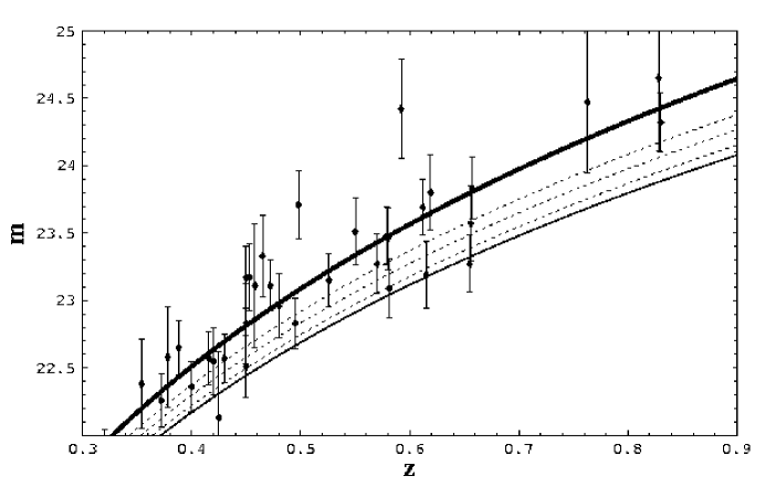
FIG. 1.: Hubble diagram for the high-redshift SNe of P99. The thick line is the best fit flat universe solution $(\Omega_{m},\Omega_{\Lambda})=(0.28,0.72)$. The thin line corresponds to $(\Omega_{m},\Omega_{\Lambda})=(1,0)$. The dotted lines are again for $(\Omega_{m},\Omega_{\Lambda})=(1,0)$ but with increasing $G$-correction, $\beta=0.1,0.3,0.5$, bottom to top.

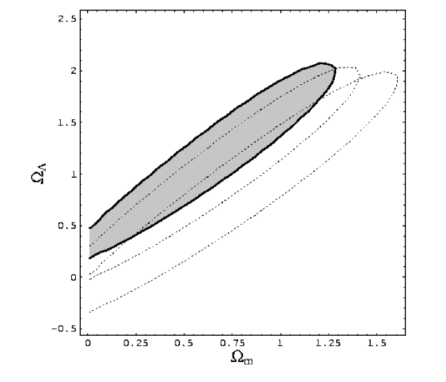
FIG. 2.: One sigma (67%) confidence regions in the plane $(\Omega_{m},\Omega_{\Lambda})$ for $\beta=0$ (shaded region) and, decreasing toward smaller $\Omega_{\Lambda}$, for $\beta=0.2$ and $\beta=0.5$.

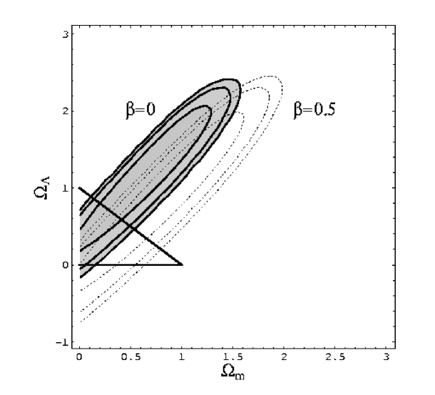
FIG. 3.: Confidence regions (67, 90 and 95%) in the plane $(\Omega_{m},\Omega_{\Lambda})$ without $G$-correction (shaded region), and with a $\beta=0.5$ $G$-correction. The straight lines correspond to a flat universe and a $\Lambda=0$ universe.

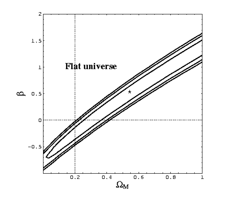
FIG. 4.: Confidence regions in the plane $(\beta,\Omega_{m})$, fixing $\Omega_{\Lambda}=1-\Omega_{m}.$ The vertical dotted line is the minimum value of $\Omega_{m}$ that is allowed observationally. The horizontal dotted line is the zero $G$-correction case. The star marks the best fit parameters.

REFERENCES

- [1] L. Amendola, Phys. Rev. D60, 043501, 1999a, astro-ph/9904120
- [2] L. Amendola, astro-ph/9906073, 1999b
- [3] L. Amendola, in preparation, 1999c
- [4] W. D. Arnett, Ap.J., 253, 785 (1982)
- [5] C. Baccigalupi, F. Perrotta & S. Matarrese, astro-ph/9906066 (1999)
- [6] R.R. Caldwell, R. Dave, & P.J. Steinhardt, Phys. Rev. Lett. 80, 1582 (1998)
- [7] X. Chen & M. Kamionkowski, astro-ph/9905368 (1999)
- [8] P.S. Drell, T. J. Loredo, & I. Wasserman, astro-ph/9905027
- [9] P. M. Garnavich et al., Ap.J., 509, 74 (1998)
- [10] S. P. Goodwin et al. astro-ph/9906187 (1999)
- [11] D. B. Guenther, L.M. Krauss & P. Demarque, Ap.J., 498, 871 (1998)
- [12] M. Morikawa, Ap.J., 369, 20 (1991)
- [13] S. Perlmutter et al. Ap.J., 517, 565 (1999)
- [14] A. G. Riess et al. Ap.J., 116, 1009 (1998)
- [15] J.-P. Uzan, Phys. Rev. D59, 123510 (1999), gr-qc/9903004,
- [16] C. Wetterich, A&A, 301, 321 (1995)
- [17] S. E. Woosley & T. A. Weaver, ARA&A, 24, 205 (1986)