A Semi-Analytic Model for Cosmological Reheating and Reionization Due to the Gravitational Collapse of Structure

Abstract

We present a semi-analytic model for the thermal and ionization history of the universe at $1000\gtrsim z\gtrsim 3$. This model incorporates much of the essential physics included in full-scale hydrodynamical simulations, such as (1) gravitational collapse and virialization; (2) star/quasar formation and subsequent ionizing radiation; (3) heating and cooling; (4) atomic and molecular physics of hydrogen; and (5) the feedback relationships between these processes. In addition, we model the process of reheating and reionization using two separate phases, self-consistently calculating the filling factor of each phase. Thus radiative transfer is treated more accurately than simulations to date have done: we allow to lowest order for both the inhomogeneity of the sources and the sinks of radiation. After calibrating and checking the results of this model against a hydrodynamical simulation, we apply our model to a variety of Gaussian and non-Gaussian CDM-dominated cosmological models. Our major conclusions include: (1) the epoch of reheating depends most strongly on the power spectrum of density fluctuations at small scales; (2) because of the effects of gas clumping, full reionization occurs at $z\sim 10$ in all models; (3) the CMBR polarization and the stars and quasars to baryons ratio are strong potential discrimants between different assumed power spectra; (4) the formation of galactic spheroids may be regulated by the evolution of reheating through feedback, so that the Jeams mass tracks the non-linear mass scale; and (5) the evolution of the bias of luminous objects can potentially discriminate strongly between Gaussian and non-Gaussian PDFs.

1 Introduction

In this paper we model semi-analytically the thermal and ionization history of the universe and its effects on the formation of luminous objects. Many parts of this complex early evolution of the universe have been studied previously, beginning with the papers of Binney (1977), Silk (1977), and Rees and Ostriker (1977), the last of whom used models of the thermal history of the universe to investigate the formation of galaxies. Tegmark et al. (1997) used a simplified model of dark matter halo profiles to derive the minimum mass of objects which are able to cool in a Hubble time. The evolution of the intergalactic medium (IGM) has been explored semi-analytically by numerous authors, including Shapiro, Giroux, and Babul (1994), and recently Valageas and Silk (1999). Also recently, Ciardi et al. (1999) use a semi-analytic model for galaxy and star formation in conjunction with high resolution N-body simulations. The detailed evolution of the IGM was addressed in a full hydrodynamical simulation by Ostriker and Gnedin (1996) and Gnedin and Ostriker (1997) (hereafter GO97). These studies explicitly allowed for clumping of the IGM, but was only able to simulate a small volume (a cube of side $2h^{-1}\mbox{Mpc}$). Ostriker and Gnedin (1996) found that a mass resolution of about $10^{4}M_{\odot}$ was required to resolve early epochs of reheating and reionization.

The more general problem of galaxy (as opposed to dark matter halo) formation has also been addressed in full hydrodynamical simulations by many investigators, including Katz, Weinberg, and Hernquist (1996), GO97, and recently by Pearce et al. (1999). Pearce et al. (1999) simulate a large volume, but with much courser mass resolution than GO97, and thus was not meant to address the details of reheating and reionization. Kauffmann, Nusser, and Steinmetz (1997) developed a “hybrid” scheme, using a semi-analytic model of gas dynamics and star formation in conjunction with N-body simulations of the formation of dark matter halos. In most cases, including all the hydrodynamical studies cited here, only Gaussian CDM have been considered.

Here, we attempt to incorporate much of the essential physics modeled by GO97 into a semi-analytic model for the reheating and reionization of the universe. The work is not explicitly three dimensional. Rather, we treat the multi-phase medium in a statistical fashion and treat collapse in the approximation of the Press-Schechter method (Press and Schechter, 1974). We consider the universe as an evolving two-phase medium — one phase ($I$) being neutral and the other phase ionized (${I\!I}$). Of course we still must make many assumptions as to which physical processes are important and which may be neglected. The main assumption we make is that UV photons from an early generation of stars and quasars are the main source of energy for the reheating and reionization of the universe

Our model also includes the following physical processes: (1) gravitational collapse and virialization, (2) non-equilibrium atomic and molecular physics of hydrogen, (3) heating and ionization by UV photons, (4) cooling, (5) simulated star/quasar formation, (6) clumping, and (7) feedback between star formation and the thermal and ionization evolution of the universe. All of these processes are calculated within the context of the standard evolution of the background cosmological model. In determining the evolution of structure formation, we explore several models for the probability density function (PDF) and power spectrum of the initial cosmological density field. Once the background cosmology and normalization of the power spectrum are fixed, our semi-analytic model has only two free parameters related to the efficiency of star formation and UV photon generation. These two parameters we fix by calibrating our results with GO97 and by requiring each cosmological scenario to reproduce appoximately the observed ionizing photon intensity $z=4$. The model we develop neglects the following processes: (1) spatial variations and correlations beyond the two phases, (2) non-virialization shock heating from gravitational collapse and supernova explosions, (3) local optical depths to UV photons and the frequency evolution of the photon energy spectrum, and (4) helium, dust, and heavy elements in the IGM. Because these effects are likely to be important at late times, we only consider our models a reasonable approximation for $z\geq 3$.

A word on motivation may be useful here. In almost all respects the full numerical hydrodynamical simulations provide a better physical treatment than we are implementing here; for example, the neglected processes (1)–(4) not treated by the current work are included in GO97. The two related ways that this treatment is to be preferred are that it is not limited by numerical resolution and that it allows, to lowest order, for a multi-phase (ionized/neutral) IGM. Given the overall relative strengths of the full numerical treatment, one can ask why bother to do anything less? The answer is threefold:

1. First, residual doubts about numerical resolution always remain whatever tests are made, so it is important to see how robust the conclusions of the numerical work are when resolution limits are removed.

2. The full numerical approach is so expensive that only a very small number of models can be explored. The result is that one is again concerned with the questions of robustness and generality of the results to variations of the adopted model. How sensitive are conclusions to the assumed nature of the perturbations (Gaussian/non-Gaussian), amplitude of the power spectrum, etc. Semianalytic methods allow one to explore the parameter space.

3. The full numerical results, paradoxically, in so far as they are better and are more and more comprehensive in physical treatment, tell one less and less! Understanding depends on knowing which physical processes and initial conditions are essential to the results, and which merely modify the details of the overall picture. A semi-analytic treatment allows one to add and subtract from the modeling to determine what matters and what does not.

The organization of this paper is as follows. In § 2, we present the elements of our adopted physical model for reheating and reionization. In § 3, we apply it to several Gaussian and non-Gaussian cosmological models. We then place some constraints on these models using several current and potential observations, such as Gunn-Peterson absorption and the CMBR, which are directly affected by the ionization history of the universe. In § 4, we discuss the relationship between the reheating and ionization history of different models to the evolution of the luminous matter in the universe. We summarize our results in § 5. In the appendices, we delineate our treatment of the standard physics of the universe, as well as the specific calculational implementation (e.g., finite difference equations) of our semi-analytic model.

2 A Model for the Physics of Reionization

In this section, we describe the semi-analytic model we use of the physics of reionization. We concentrate on the treatment of a two-phase medium with sources and sinks of radiation. In particular we define our basic differential equations, and describe how we calculate the formation rate of bound objects, the UV production rate, and the clumping of cosmic gas.

2.1 Definitions and Conservation Equations

Since we are considering a two-phase medium, we will need to understand the time evolution of the filling factor of ionized regions $f_{{I\!I}}$. The two other independent quantities required are the ionization fraction in the ionized region $x_{{I\!I}}$ and the mean (volume-averaged) UV ionizing ($\geq 13.6$ eV $\equiv\epsilon_{0}$) intensity $\bar{J}$. The corresponding intensity in the ionized region is $\bar{J}_{{I\!I}}=\bar{J}/f_{{I\!I}}$. In our notation, $n_{H}$ is the total mean hydrogen density.

Considering only ionization of hydrogen, local particle conservation in the ionized region gives

$$\frac{d}{dt}\left(n_{H}x_{{I\!I}}\right) = -3\frac{\dot{a}}{a}n_{H}x_{{I\!I}}+n_{H}(1-x_{{I\!I}})\frac{4\pi\bar{J}_{{I\!I}}\sigma_{p}}{\epsilon_{0}}$$ (2)

$$\qquad+\,{\cal C}\,n_{H}^{2}\left[x_{{I\!I}}(1-x_{{I\!I}})k_{ci}-x_{{I\!I}}^{2}\alpha_{R}\right]$$

$$= -3\frac{\dot{a}}{a}n_{H}x_{{I\!I}}+n_{H}(1-x_{{I\!I}})\frac{\bar{E}c\sigma_{p}}{f_{{I\!I}}\epsilon_{0}}$$

$$\qquad+\,{\cal C}\,n_{H}^{2}\left[x_{{I\!I}}(1-x_{{I\!I}})k_{ci}-x_{{I\!I}}^{2}\alpha_{R}\right]$$

where the first term on the right hand side is from the expansion of the universe, and the second term from photoionization, and the third term from collisional ionizations (rate coefficient $k_{ci}$) and radiative recombinations (rate coefficient $\alpha_{R}$). The effective cross section to photoionization $\sigma_{p}$ is given below. The clumping factor ${\cal C}\equiv\langle\rho_{b}^{2}\rangle/\langle\rho_{b}\rangle^{2}$ takes into account the non-uniformity of the gas. We describe how to estimate ${\cal C}$ in § 2.4.

For an energy spectrum of the form $E_{\nu}\propto\nu^{-\gamma}$, the average UV energy density ($E=4\pi J/c$) of the universe evolves as

$$\frac{d\bar{E}}{dt} = \bar{S}-[4+(\gamma-1)]\frac{\dot{a}}{a}\bar{E}-f_{{I\!I}}n_{H}(1-x_{{I\!I}})4\pi\bar{J}_{{I\!I}}\sigma_{e}-\epsilon_{0}n_{H}x_{{I\!I}}\frac{df_{{I\!I}}}{dt}$$ (3)

$$= \bar{S}-[4+(\gamma-1)]\frac{\dot{a}}{a}\bar{E}-n_{H}(1-x_{{I\!I}})\bar{E}c\sigma_{e}-\epsilon_{0}n_{H}x_{{I\!I}}\frac{df_{{I\!I}}}{dt},$$ (4)

where we have used the relationship between $\bar{E}$, $\bar{E}_{{I\!I}}$, and $\bar{J}_{{I\!I}}$. We use a value of $\gamma=1.5$ throughout. The integrated source function is given by $\bar{S}$, the Hubble expansion is accounted for in the second term, energy lost to maintaining the ionization of the ionized region is given by the third term, and the last term is due to energy lost to ionizing new (i.e., previously neutral) material. The effective UV energy loss cross section is $\sigma_{e}$.

The definitions of $\sigma_{p}$ and $\sigma_{e}$ are as follows. If the ionizing specific intensity is $\bar{J}_{\nu}$, then the ionizing intensity is

$$\bar{J}\equiv\int_{\nu_{0}}^{\nu_{\ast}}\bar{J}_{\nu}d\nu,$$ (5)

where $\nu_{\ast}$ is a high frequency cutoff (we use 7.4 keV, from Abel 1998). For a power law

$$\bar{J}_{\nu}=J_{0}\nu_{0}^{-1}\left(\frac{\nu_{0}}{\nu}\right)^{\gamma},$$ (6)

we have the relation

$$\bar{J}=\frac{J_{0}}{\gamma-1}\left[1-\left(\frac{\nu_{0}}{\nu_{\ast}}\right)^{\gamma-1}\right].$$ (7)

The photoionization rate per hydrogen atom is given (in s^-1) by

$$\Gamma_{p} \equiv \int_{\nu_{0}}^{\nu_{\ast}}4\pi\bar{J}_{\nu}\sigma(\nu)\frac{d\nu}{h_{p}\nu}$$ (8)

$$= \frac{4\pi J_{0}}{h_{p}\nu_{0}}\int_{\nu_{0}}^{\nu_{\ast}}\left(\frac{\nu_{0}}{\nu}\right)^{\gamma}\sigma(\nu)\frac{d\nu}{\nu},$$ (9)

where $h_{p}$ is Planck’s constant. Equating this with $4\pi\bar{J}\sigma_{p}/\epsilon_{0}$ gives

$$\sigma_{p}\equiv\frac{\gamma-1}{1-\left(\frac{\nu_{0}}{\nu_{\ast}}\right)^{\gamma-1}}\int_{\nu_{0}}^{\nu_{\ast}}\left(\frac{\nu_{0}}{\nu}\right)^{\gamma}\sigma(\nu)\frac{d\nu}{\nu}.$$ (10)

Similarly, assuming that all the excess energy from each photoionization goes into heat and produces no UV photons, the rate of UV energy loss per hydrogen atom (erg s^-1) is

$$\Gamma_{e} \equiv \int_{\nu_{0}}^{\nu_{\ast}}4\pi\bar{J}_{\nu}\sigma(\nu)d\nu$$ (11)

$$= 4\pi J_{0}\int_{\nu_{0}}^{\nu_{\ast}}\left(\frac{\nu_{0}}{\nu}\right)^{\gamma}\sigma(\nu)\frac{d\nu}{\nu_{0}}.$$ (12)

Equating this with $4\pi\bar{J}\sigma_{e}$ gives

$$\sigma_{e}\equiv\frac{\gamma-1}{1-\left(\frac{\nu_{0}}{\nu_{\ast}}\right)^{\gamma-1}}\int_{\nu_{0}}^{\nu_{\ast}}\left(\frac{\nu_{0}}{\nu}\right)^{\gamma}\sigma(\nu)\frac{d\nu}{\nu_{0}}.$$ (13)

The difference between these cross sections gives the cross section for photoheating, or equivalently a photoheating rate (erg s^-1) of

$$\Gamma_{ph}\equiv 4\pi\bar{J}(\sigma_{e}-\sigma_{p}).$$ (14)

In order to fully specify the model, we need to be able to determine $\bar{S}$, as well as have a relationship between $\bar{E}$ and $f_{{I\!I}}$. These turn out to be intimately related.

2.2 Formation Rate of Bound Objects

We assume that stars/quasars only form in virialized collapsed objects. Hence the first input into the star formation rate is the formation rate of bound objects. In the next subsection we relate these bound objects to UV energy output in order to derive expressions for the source function $\bar{S}$ and the relationship between the mean radiation energy density $\bar{E}$ and the filling factor $f_{{I\!I}}$.

Generalized Press-Schechter for a PDF $P(\nu)$, and normalization factor $f^{-1}\equiv\int_{0}^{\infty}P(\nu)d\nu$ gives the comoving number density of collapsed objects with initial comoving radius between $R$ and $R+dR$ to be

$$N_{R}dR = f\cdot P\left[\nu(R,t)\right]\frac{3}{4\pi R^{3}}\frac{\partial\ln\nu(R,t)}{\partial\ln R}\nu(R,t)\frac{dR}{R}$$ (15)

$$\nu(R,t) \equiv \frac{\delta_{c}}{\sigma(R)\,D(t)}$$ (16)

$$\frac{\partial\ln\nu(R,t)}{\partial\ln R} = \frac{d\ln\sigma^{-1}(R)}{d\ln R}\equiv\alpha(R)$$ (17)

where $\sigma(R)$ is the rms fluctuation on scale $R$ linearly extrapolated to the present, $\delta_{c}\approx 1.69$ is the standard linear overdensity of collapse, and $D(t)$ is the linear growth factor normalized to $D(t_{0})=1$. The original Press-Schechter (Press and Schechter, 1974) method was derived in for a Gaussian PDF, and has been checked in that case with N-body simulations (Efstathiou et al., 1988). These expressions in the non-Gaussian case were derived in Chiu, Ostriker, and Strauss (1997), and recently tested through N-body simulations for several non-Gaussian models (Robinson and Baker, 1999).

For each model, we filter the power spectrum using a top-hat window to obtain the rms fluctuation $\sigma$. The power spectra we use are from Bardeen et al. (1986) and Sugiyama (1995) in the adiabatic cases; Pen, Spergel, and Turok (1994) and Pen and Spergel (1995) in the textures case; and Peebles 1999ab in the ICDM case.

In general, we cannot use only the Press-Schechter number density to determine the formation rate of bound objects. This is because the net time-rate of change of the number density of objects at a particular scale consists of both a formation $\dot{N}_{R,\rm form}$ rate and a destruction rate $\dot{N}_{R,\rm dest}$. Thus the actual formation rate may be larger than the rate inferred from Press-Schecter alone. Of course, we must constrain these rates to be consistent with the Press-Schechter formalism:

$$\dot{N}_{R}=\dot{N}_{R,\rm form}-\dot{N}_{R,\rm dest},$$ (18)

where $\dot{N}_{R}$ is given by differentiating equations (15)–(17) with respect to time. We seek a semi-analytic methodology applicable to an arbitrary PDF which gives these two rates.

Sasaki (1994) models the formation and destruction rates of these objects by assuming that the destruction efficiency rate $\phi\equiv\dot{N}_{R,\rm dest}/N_{R}$ has no characteristic scale — “destruction” by incorporation into larger objects is hierarchical and scale-invariant. In this section, we generalize his derivation to non-Gaussian PDFs.

The assumption of no characteristic scale of destruction efficiency, in addition to the requirement that the net rate of formation minus destruction be consistent with Press-Schechter, leads to the conclusion that $\phi$ must be a function only of time. Sasaki (1994) derives the following relation for the destruction probability per unit time:

$$\phi(t)=\frac{\dot{D}}{D},$$ (19)

which we find to be independent of the PDF. It follows that the probability that an object created at $t_{1}$ exists at $t_{2}$ without having been incorporated into a larger object is given by

$$p_{\rm surv}(t_{2}|t_{1})=\exp\left[\int_{t_{1}}^{t_{2}}\phi(t)dt\right]=\frac{D(t_{1})}{D(t_{2})}.$$ (20)

Combining $\phi$ and the Press-Schechter consistency requirement equation (18) leads to a formation rate of the form:

$$\dot{N}_{R,\rm form}=N_{R}\cdot\nu(R,t)\frac{\dot{D}}{D}\left(\frac{-P^{\prime}}{P}\right),$$ (21)

where $P^{\prime}=dP/d\nu$. The quantity $-P^{\prime}/P$ for a Gaussian and an exponential $P(\nu)$ takes on the forms:

$$\frac{-P^{\prime}}{P} = \nu,\qquad\mbox{if}\ P(\nu)\propto e^{-\frac{1}{2}\nu^{2}};$$ (22)

$$\frac{-P^{\prime}}{P} = \omega,\qquad\mbox{if}\ P(\nu)\propto e^{-\omega\nu}.$$ (23)

Textures and non-Gaussian ICDM both have PDFs which are well approximated by exponentials (Gooding et al. 1992; Park, Spergel, & Turok 1991; Peebles 1998ab). For textures $\omega=1.45$ (using Park, Spergel, & Turok 1991 as described in Chiu, Ostriker, & Strauss 1997), and for non-Gaussian ICDM $\omega=0.67$ Peebles (1999b). Recalling that

$$\frac{\dot{D}}{D}=f(\Omega)\frac{\dot{a}}{a},$$ (24)

where the velocity factor $f(\Omega)\approx\Omega^{0.6}$, the formation rate in closed form is

$$\dot{N}_{R,\rm form}dR=f\cdot\left[-P^{\prime}(\nu)\right]\frac{3}{4\pi R^{3}}f(\Omega)\frac{\dot{a}}{a}\alpha(R)\,\nu^{2}(R,t)\,\frac{dR}{R}.$$ (25)

This is the formation rate per comoving volume we use in our model. For a power law $\sigma(R)\propto R^{-\alpha}$, the logarithmic slope $\partial\ln\nu/\partial\ln R=\alpha$ is a constant.

This formalism for merging and formation rates is consistent with the work of Blain and Longair (1993), who used a numerical extension of Press-Schechter with simple forms for the merging probability. All other work of this type is based on Lacey and Cole (1993) and Lacey and Cole (1994), who construct conditional probabilities by extending the work of Bond et al. (1991). Unfortunately, this method is heavily dependent upon the PDF begin Gaussian, and is sufficiently complicated so that extending it to non-Gaussian PDF is not straight forward. Furthermore, since objects are “constantly growing” in the Lacey and Cole (1993) formalism, rather than in “punctuated equilibrium” as implied by equation (20), it is difficult to directly compare the two methods. However, one sign that they might be roughly consistent is that Viana and Liddle (1996) obtain similar results for cluster abundances whether they use the Lacey and Cole (1993) or the Sasaki (1994) methodology.

We further note that during reheating and reionization, structure formation is largely hierarchical in most of the models we consider. This is because only a small fraction of the universe needs to collapse in order to release enough energy in order to reheat and reionize the universe. Collapsed objects are thus still “rare” ($\nu>1$), and their net formation rates are thus dominated by their creation rates. The use of the Sasaki results thus provide only a small correction. In the limit where the “destruction” rates are negligible, all semi-analytic merging formalisms which are based on Press-Schechter must give the same answer in order to be consistent with equation (18).

2.3 Determining the UV Production Rate

Our basic model for UV production is that individual halos which can undergo star formation will emit UV radiation radially, and thus be surrounded by a sphere of ionized material, a “cosmological Strömgren sphere.” Consider halos of baryonic mass in the range $M_{b}$ to $M_{b}+dM_{b}$, corresponding to comoving length scale between $R$ and $R+dR$, formed in the time interval $\tilde{t}$ to $\tilde{t}+d\tilde{t}$, and “observed” at time $t$. The comoving number density of such objects is given by

$$N(R,\tilde{t},t)\,dR\,d\tilde{t}=\dot{N}_{\rm form}(R,\tilde{t})\cdot p_{\rm surv}(t|\tilde{t})\,dR\,d\tilde{t},$$ (26)

where the notation is the same as in the previous section. The second factor accounts for the destruction objects of scale $R$ through merging into larger objects. Although we are using Sasaki’s method to determine $\dot{N}_{\rm form}$ and $p_{\rm surv}$ as described above, the form of equation (26) is completely general. Note that $M_{b}$ and $R$ are related by $M_{b}=4\pi R^{3}\rho_{b,0}/3$. Following the prescriptions of Cen (1992) and Gnedin (1996), we assume that star formation is spread over a dynamical time scale, so that the UV luminosity of such an object is given by

$$\ell(M_{b},\tilde{t},t)=(1-f_{\ast})M_{b}c^{2}\frac{\epsilon_{\rm cool}\epsilon_{\ast}\epsilon_{\rm hm}\epsilon_{\rm UV}}{\tilde{t}_{\rm dyn}}\left(\frac{t-\tilde{t}}{\tilde{t}_{\rm dyn}}\right)\exp\left[-\left(\frac{t-\tilde{t}}{\tilde{t}_{\rm dyn}}\right)\right],$$ (27)

where $f_{\ast}$ is the fraction of the baryonic mass which has already been processed into stars/quasars and $\tilde{t}_{\rm dyn}$ is the dynamical time associated with the object at its time of formation (see equation C1). We are also assuming here that the stars/quasars are uniformly distributed throughout the collapsed halo.

The efficiencies $\epsilon_{i}$ are as follows: $\epsilon_{\rm cool}$ is the mass fraction of the halo which is cooling, $\epsilon_{\ast}$ is the mass fraction of cooling gas which physically ends up in collapsed objects, $\epsilon_{\rm hm}$ is the mass fraction of collapsed objects which are quasars or high-mass stars (i.e., with substantial UV flux), and $\epsilon_{\rm UV}$ is the mass-to-UV efficiency of the high-mass stars/quasars. The cooling fraction $\epsilon_{\rm cool}$ we derive below in Appendix C, and is a function of the halo virial mass and the redshift of collapse. GO97 uses $\epsilon_{\rm UV}=6\times 10^{-5}$ and Gnedin (1996) gives $\epsilon_{\rm hm}=0.16$, derived using a standard initial mass function. We cannot use $\epsilon_{\rm UV}$ directly because we are not resolving the mass elements within individual cooling halos. The “resolution” factor $\epsilon_{\ast}$ parameterizes this uncertainty. We use a net efficiency

$$\epsilon_{\rm eff}\equiv\epsilon_{\ast}\epsilon_{\rm hm}\epsilon_{\rm UV},$$ (28)

normalized by requiring, for each model, that the ionizing intensity $J_{21}=1$ at $z=4$. There is, effectively, only one free parameter here, $\epsilon_{\rm eff}$, and that is fixed by normalizing to observations.

A separate estimate of $\epsilon_{\ast}$, however, is necessary in order to derive $f_{\ast}$, the fraction of baryons which is sequestered in stars/quasars and their remnants. It is important to keep track of $f_{\ast}$ to avoid “double counting” star formation — baryons which are in such bound objects are not available for additional star formation. Note that results are insensitive to the value of $f_{\ast}$ while $f_{\ast}\lesssim 10\%$, since they are only dependent on $1-f_{\ast}$. We can use the GO97 simulation to derive our “resolution” factor $\epsilon_{\ast}$ by assuming that it is constant for all cosmological models. If $\epsilon_{\ast}$ is a constant, then it should correspond to the value which gives the same $J_{21}$ as the GO97 simulation, using their values for $\epsilon_{\rm hm}$ and $\epsilon_{\rm UV}$ and the same cosmological model. This correspondence leads to a value $\epsilon_{\ast}\approx 0.5$.

Given $\epsilon_{\ast}$, the simplest way to calculate the fraction $f_{\ast}$ is actually to integrate over the UV production rate $\bar{S}$, given in equation (31), dividing by the appropriate efficiencies:

$$f_{\ast}(t) = \int_{0}^{t}\frac{\bar{S}(\tilde{t})d\tilde{t}}{\epsilon_{\rm hm}\epsilon_{\rm UV}n_{H}m_{H}c^{2}/X}$$ (29)

$$= \epsilon_{\ast}\int_{0}^{t}\frac{\bar{S}(\tilde{t})d\tilde{t}}{\epsilon_{\rm eff}n_{H}m_{H}c^{2}/X},$$ (30)

where $X$ is the hydrogen mass fraction, and we have expressed the result in terms of the $J_{21}$-normalized effective efficiency $\epsilon_{\rm eff}$ and the resolution factor $\epsilon_{\ast}$. As a check on our value of $\epsilon_{\ast}$, we compare $f_{\ast}$ at $z\approx 4$ between our model and the GO97 simulation, given the same cosmological parameters. We find the values to be consistent, with $f_{\ast}\approx 2\%$ at this redshift (see also Figure A Semi-Analytic Model for Cosmological Reheating and Reionization Due to the Gravitational Collapse of Structure).

The global mean UV production rate per unit (physical) volume is given by

$$\bar{S}(t)=a(t)^{-3}\int_{0}^{\infty}dR\int_{0}^{t}d\tilde{t}\,\psi(R,\tilde{t})\cdot N(R,\tilde{t},t)\cdot\ell(M_{b},\tilde{t},t),$$ (31)

where the function $\psi(R,\tilde{t})$ is a selection function for objects which are able to collapse and form stars/quasars. One simple form for $\psi$ is

$$\psi_{\rm simp}(R,\tilde{t})=\theta[R-R_{J}(\tilde{t})],$$ (32)

where the $\theta$ function is zero if the argument is $<0$ and unity if the argument is $>0$. These represent the criteria that a mass must be greater than the Jeans mass to collapse. In order to account for the fact that the Jeans mass will be different in the two phases, we can define $\psi$ to be

$$\psi_{\rm 2ph}(R,\tilde{t})=\left\{(1-\tilde{f}_{{I\!I}})\cdot\theta\left[R-R_{J,c}(\tilde{t})\right]+\tilde{f}_{{I\!I}}\cdot\theta\left[R-R_{J,h}(\tilde{t})\right]\right\},$$ (33)

where $\tilde{f}_{{I\!I}}$ is the filling factor of the ionized region at time $\tilde{t}$, $M_{J,c}$ is the Jeans mass in the neutral (cold) region, and $M_{J,h}$ is the Jeans mass in the ionized (hot) region. Note that we are assuming that an object, once formed, can only be destroyed by merging and forming a larger object. We are assuming, thus, that virialized gas halos are “self-shielded” from ionizing radiation due to their high density. That is, they can not be heated to the point of dynamical instability nor can they be “evaporated” away.

In order to derive the needed relation between $f_{{I\!I}}(t)$ and $\bar{E}(t)$, we make two further assumptions. One is that the ionized volume $v_{{I\!I}}(M_{b},\tilde{t},t)$ around an isolated object is proportional to its UV luminosity $\ell(M_{b},\tilde{t},t)$ with a coefficient of proportionality $\kappa(t)$ that is a function only of the time $t$ when it is “observed.” This should be a reasonable approximation, since the recombination rates are determined by the density and temperature at $t$, not at the formation time $\tilde{t}$. As long as objects live longer than the recombination time, our assumption is consistent with the work of Shapiro and Giroux (1987) on cosmological H II regions. We thus have the relation

$$\ell(M_{b},\tilde{t},t)=\kappa^{-1}(t)\,v_{{I\!I}}(M_{b},\tilde{t},t)\equiv\frac{4\pi}{3\kappa(t)}r_{{I\!I}}^{3}.$$ (34)

The second assumption, which is needed to determine $\kappa(t)$ from $f_{{I\!I}}(t)$ and $\bar{S}(t)$, is that the filling factor can be related to the average number of “overlapping” ionized regions by modeling it as an uncorrelated Poisson process. The average number $\lambda(t)$ of overlapping regions seen by a random volume element is

$$\lambda(t)\equiv\int_{0}^{\infty}dR\int_{0}^{t}d\tilde{t}\,\psi(R,\tilde{t})\cdot N(R,\tilde{t},t)\cdot v_{{I\!I}}(M_{b},\tilde{t},t).$$ (35)

We no longer have the factor $a^{-3}$ because $v_{{I\!I}}$ is a comoving volume. For Poisson probabilities, the filling factor $f_{{I\!I}}(t)$ is related to $\lambda(t)$ by

$$f_{{I\!I}}(t)=1-e^{-\lambda(t)}.$$ (36)

Combining equation (35) with equation (34) and using (31) gives

$$\lambda(t)=\kappa(t)\,a^{3}(t)\,\bar{S}(t).$$ (37)

Thus we have determined $\kappa(t)$ in terms of $f_{{I\!I}}(t)$ and $\bar{S}(t)$.

With $\kappa(t)$ defined, we can derive a relationship between $f_{{I\!I}}(t)$ and $\bar{E}(t)$ which will close our system of equations. Consider the contribution of each source to the mean intensity $\bar{J}(t)$. Neglecting the optical depth within an isolated ionized region, and assuming no flux escapes beyond a radius $r_{{I\!I}}(M_{b},\tilde{t},t)$, the average flux seen by a random volume element due to an object of luminosity $\ell(M_{b},\tilde{t},t)$ is

$$d[4\pi\bar{J}(t)] = dR\,d\tilde{t}\,N(R,\tilde{t},t)\int_{0}^{r_{{I\!I}}}d^{3}r\frac{\ell(M_{b},\tilde{t},t)}{4\pi[a(t)\,r]^{2}}$$ (38)

$$= dR\,d\tilde{t}\,N(R,\tilde{t},t)\cdot\ell(M_{b},\tilde{t},t)\cdot r_{{I\!I}}(M_{b},\tilde{t},t)\cdot a^{-2}(t)$$ (39)

$$= dR\,d\tilde{t}\,N(R,\tilde{t},t)\cdot\ell^{4/3}(M_{b},\tilde{t},t)\left[\frac{3\kappa(t)}{4\pi}\right]^{1/3}a^{-2}(t),$$ (40)

where $r$ is a comoving length, $a\,r$ is a physical length, and we have used

$$r_{{I\!I}}(M_{b},\tilde{t},t)=\left[\frac{3\kappa(t)}{4\pi}\ell(M_{b},\tilde{t},t)\right]^{1/3},$$ (41)

which we assume to be much smaller than the Hubble radius. Equation (40) also assumes that the central luminous object emits radiation radially, which is a good approximation as long as the radius of the sphere is much larger than the virial radius. Using equation (37) in equation (40) gives

$$d(4\pi\bar{J})=dR\,d\tilde{t}\,N(R,\tilde{t},t)\cdot\ell^{4/3}(M_{b},\tilde{t},t)\left[\frac{3\lambda(t)}{4\pi\bar{S}(t)}\right]^{1/3}a^{-3}(t).$$ (42)

Therefore the mean energy density $\bar{E}(t)=4\pi\bar{J}(t)/c$ at time $t$ is given by

$$\bar{E}(t)=\frac{1}{c}\left[\frac{3\lambda(t)}{4\pi\bar{S}(t)}\right]^{1/3}a^{-3}\int_{0}^{\infty}dR\int_{0}^{t}d\tilde{t}\,\psi(R,\tilde{t})\cdot N(R,\tilde{t},t)\cdot\ell^{4/3}(M_{b},\tilde{t},t).$$ (43)

This is the desired relationship between $f_{{I\!I}}(t)=(1-e^{-\lambda(t)})$ and $\bar{E}(t)$ which closes the system of equations.

We have neglected spatial correlations among these sources. This approximation should be less important for the texture model, which is well approximated by uncorrelated seeds, than for the Gaussian models. As long as the filling factor is small, though, these correlations are likely not to be important, since most of the universe is neutral. We will find below that in the Gaussian cases we consider, reionization occurs quite rapidly, and this rapid percolation likely overwhelms any spatial correlations, which tend to slow down the percolation.

Furthermore, we have neglected the optical depths within the collapsed object as well as in the gas in the Strömgren sphere surrounding each object. We assume both that the covering factor of other halos within the sphere is small, and that there is a sharp transition between the ionized and neutral regions. This approximation is somewhat alleviated by assuming a clumping factor for the gas (see § 2.4). With clumping, our model is self-consistent in the volume average, accounting for all photoionizations and recombinations in the ionized region.

In summary, we assume that star formation in collapsed halos is the source of UV photons. The number density of these sources is determined using the Press-Schechter formalism with the requirement that the baryonic halo mass is greater than the Jeans mass; the luminosity of each source is determined by the fraction of cooling gas and several efficiency factors. These sources are assumed to be scattered randomly (i.e., a Poisson point process), and each surrounded by a Strömgren sphere. The volume emmissivity of these objects is assumed to be uniform, and they are assumed to radiate radially into the surrounding intergalactic medium. Assuming that at fixed time, the volume of each Strömgren sphere is proportional to the luminosity of the central source, the radius of each sphere is determined by requiring consistency among the filling factor, the mean intensity, the number density of sources, and the total UV luminosity.

2.4 Nonuniformity of Cosmic Gas: The Clumping Factor and Tracking the Diffuse Component

The importance of clumping in determining the ionization history of the universe was stressed by GO97. Because the clumping factor has been neglected in most previous semi-analytic work on reionization, there has been no attempt to estimate it analytically. In this subsection we use Press-Schechter to estimate the clumping factor. A similar procedure was described in Valageas and Silk (1999).

Consider dividing the baryons in the universe into clumped and diffuse components. The clumped component consists of baryons which have collapsed into virialized halos. Using equation (26), the fraction of the baryonic mass of the universe which collapsed $df_{m}$ in time interval $\tilde{t}$ to $\tilde{t}+d\tilde{t}$, and survives without being incorporated into a larger object to time $t$, is given by

$$df_{m}(\tilde{t})\equiv\left[\int dR\,\frac{D(\tilde{t})}{D(t)}\dot{N}_{\rm form}(R,\tilde{t})\frac{4\pi R^{3}}{3}\,\psi(R,\tilde{t})\right]\,d\tilde{t},$$ (44)

where $\psi(R,\tilde{t})$ is the selection function which filters out objects below the Jeans scale. The fraction of baryonic mass which is in collapsed objects at time $t$ is given by integrating over $\tilde{t}$:

$$f_{m}(t)=\int^{t}\frac{df_{m}(\tilde{t})}{d\tilde{t}}d\tilde{t}.$$ (45)

Note that we do not take the collapsed fraction $f_{m}(t)$ to be equal to be the fraction of mass above the Jeans mass at time $t$. This is because during reheating, the Jeans mass increases, but objects below the Jeans mass which formed at earlier times (when the Jeans mass was lower) can still survive as long as they are not merged into larger objects. If all of these objects are in virialized halos, then their overdensity relative to the mean density will by

$$\frac{\rho_{\rm vir}}{\bar{\rho}}\equiv\bar{\delta}_{\rm vir}\equiv\frac{\Delta_{\rm vir}}{\Omega(t)},$$ (46)

where $\Delta_{\rm vir}$ is the overdensity relative to the critical density. Thus the fraction of the volume in the universe that they occupy will be

$$f_{v}(t)=\frac{f_{m}}{\bar{\delta}_{\rm vir}}.$$ (47)

Self-consistency requires that the diffuse component be underdense so that $\rho_{\rm diff}<\bar{\rho}$. Taking volume average gives

$$\bar{\rho}=f_{v}\rho_{\rm vir}+(1-f_{v})\rho_{\rm diff},$$ (48)

which implies that

$$\frac{\rho_{\rm diff}}{\bar{\rho}}=\frac{1-f_{m}}{1-f_{v}}.$$ (49)

The volume-averaged square density will be

$$\langle\rho^{2}\rangle = f_{v}\rho_{\rm vir}^{2}+(1-f_{v})\rho_{\rm diff}^{2}$$ (50)

$$= \bar{\rho}^{2}\left(f_{m}\bar{\delta}_{\rm vir}+\frac{(1-f_{m})^{2}}{1-f_{v}}\right).$$ (51)

The average clumping factor ${\cal C}$ is thus

$${\cal C} \equiv \langle\rho^{2}\rangle/\bar{\rho}^{2}$$ (52)

$$= f_{m}\bar{\delta}_{\rm vir}+\frac{(1-f_{m})^{2}}{1-f_{v}}.$$ (53)

This is the clumping factor we use in our model. Our model, however, assumes that UV sources are uniformly distributed throughout collapsed halos and that all halos carry the same overdensity. These two assumptions will tend to reduce clumping, so equation (53) probably gives a lower bound on the importance of clumping. As shown in Figure A Semi-Analytic Model for Cosmological Reheating and Reionization Due to the Gravitational Collapse of Structure, the results of this semi-analytic calculation are in fair agreement with the results of the numerical simulation in GO97.

We keep track of the ionization and temperature history of the purely diffuse phase of the ionized region. We do this in order to properly calculate the Gunn-Peterson optical depth, which probes the diffuse intergalactic medium (IGM). This phase is by definition unclumped, and is underdense relative to the mean, equation (49). Note, however, that this diffuse phase plays no feedback role — it simply responds to the other physics which is going on.

3 Results

In this section we present the results of our calculations for a range of cosmological models. We begin with a “calibration” model which uses the same cosmological parameters as were used by GO97 ($\Omega_{0}=0.35$, $\Omega_{\Lambda}=0.65$, $h=0.70$, and $\Omega_{b}=0.03$). We then consider adiabatic Gaussian CDM (G+ACDM), textures (T+CDM), and non-Gaussian isocurvature CDM (ICDM) as proposed by Peebles (1999ab). To help assess the sensitivity of the results to the PDF and the power spectrum, we also consider an “artificial” case of a texture PDF with an adiabatic CDM power spectrum (T+ACDM). We use a Hubble parameter $h=0.65$, a baryon density parameter $\Omega_{b}h^{2}=0.0125$ throughout, and consider flat ($\Lambda$-dominated) and open models with matter density parameters of $\Omega_{0}=$ 1, 0.45, 0.35, and 0.25. All models are normalized to cluster abundances (method of Chiu, Ostriker, & Strauss 1997 for all models except ICDM, which uses Peebles 1999ab). The cosmological parameters associated with the models we consider are listed in the first three columns of Table 1. As noted above, the UV efficiency $\epsilon_{\rm eff}$ in each run is adjusted to reproduce $J_{21}=1$ at $z=4$. There are no other adjustable parameters in the model.

3.1 Comparison with GO97 Simulation

In Figure A Semi-Analytic Model for Cosmological Reheating and Reionization Due to the Gravitational Collapse of Structure we show the filling factor $f_{{I\!I}}$, the ionizing intensity $J_{21}$, the neutral fraction $\langle 1-x\rangle$, and the gas temperature $T$ in the case were we mimic the GO97 calculation. While the ionizing intensity was adjusted to be consistent with the GO97 value at $z=4$, the evolution of $J_{21}$ is similar in the two calculations. As in the GO97 calculation, reionization to $1-x=10^{-3}$ occurs suddenly at $z\sim 10$, while reheating occurs more gradually. The main difference between this work and GO97 is that reionization and reheating begin somewhat earlier in our model. This may in part be due to the limited resolution and single-phase treatment of GO97.

In Figure A Semi-Analytic Model for Cosmological Reheating and Reionization Due to the Gravitational Collapse of Structure, we show the stellar fraction and clumping factor for this reionization calculation. Again, the values are similar to those in GO97. The clumping factor shows the greatest discrepancy, and is without doubt inaccurately calculated in our model. Without full-scale simulation, however, it is difficult to calculate the clumping factor to a much greater accuracy than what we have presented in § 2.4. The fact that our result is within a factor of a few of the GO97 calculation is encouraging. The earlier onset of star formation shown in the top panel by our semi-analytic model may reflect the limited resolution of GO97, which while adequate for average objects, is insufficient for early, dense small ones.

In Figure A Semi-Analytic Model for Cosmological Reheating and Reionization Due to the Gravitational Collapse of Structure, we show the nonlinear and average Jeans mass scales derived from our model. Our results are qualitatively consistent with OG96: we find that the Jeans mass and the nonlinear mass (here defined by $\delta M/M\approx 0.4$) track each other to remarkable accuracy during the reheating phase. Because reheating begins earlier in this model than in the GO97 simulation, the precise degree of nonlinearity which tracks the Jeans mass is different, and the epochs during which the Jeans and nonlinear mass scales track each other occur earlier. A possible physical basis for this tracking is clear. When the Jeans mass is lower than the nonlinear mass, star formation accelerates so that the average temperature increases, the Jeans mass increases to above the nonlinear mass scale, and further star formation is quenched.

We do not expect an exact correspondence between our method and the GO97 work. For example, this semi-analytic calculation is not limited by mass resolution, so mass condensations down to the Jeans mass limit can contribute to the ionizing UV flux. This may partially explain why reheating starts at $z\sim 30$ in our model, rather than at $z\sim 20$ in GO97. Another contributing factor to this difference in the reheating epoch is that the largest GO97 simulation lacked significant large-scale power relative to the true power spectrum. Furthermore, we model here a two-phase medium where the radiation field is not spatially uniform, while GO97 use an average UV radiation field. On the other hand, this calculation neglects all spatial correlations, which are automatically taken into account by the three-dimensional numerical calculation of GO97, and uses a power-law radiation spectrum. While it is unclear what the net effect of all these differences should be, it is encouraging that two completely different methods of calculating the reheating and reionization of the universe give such similar results.

3.2 Reheating and Reionization in Various Cosmologies

The results of our calculations for the models we consider are presented in Table 1 and Figures A Semi-Analytic Model for Cosmological Reheating and Reionization Due to the Gravitational Collapse of Structure–A Semi-Analytic Model for Cosmological Reheating and Reionization Due to the Gravitational Collapse of Structure. Qualitatively, the evolution of reheating and reionization can be divided into two broad categories characterized by late or early reheating, corresponding to late or early evolution of the filling factor $f_{{I\!I}}$. In models with late reheating, which include the Gaussian models and the T+ACDM model, the filling factor rises from $f_{{I\!I}}<10^{-4}$ at $z=30\sim 50$ to $f_{{I\!I}}\sim 1$ at $z=10\sim 20$. For models with early reheating, which include the pure texture T+CDM models and the ICDM model, the filling factor is already $f_{{I\!I}}>0.1$ at $z\sim 80$, but rises slowly to $f_{{I\!I}}=1$ at $z=10\sim 20$.

The general picture of the evolution in these models is as follows. We note that by “reionization” we mean when $f_{{I\!I}}$ is approaching unity, but that by “full reionization” we mean the epoch at which the individual ionized regions start overlapping substantially, so that $\lambda=-\ln{(1-f_{{I\!I}})}\gg 1$.

For an adiabatic CDM-type power spectrum, the fluctuation spectrum $\sigma_{R}$ rises logarithmically, or nearly logarithmically, as $R\rightarrow 0$. Hence, at the Jeans scale of $\sim 0.01h^{-1}\mbox{Mpc}$, there is a logarithmic cutoff in power for $z>\sigma_{R_{J}}\sim 10-20$. Furthermore, cooling becomes less efficient at the Jeans scale at later times. These two factors lead to a suppression of reheating and reionization until late times. Full reionization occurs after the filling factor approaches unity, at redshifts $z\lesssim 10$.

These results for Gaussian CDM models are consistent with the work of GO97 (who considered a flat $\Omega_{\Lambda}=0.35$ CDM model), as well as Ciardi et al. (1999) (who considered an $\Omega_{0}=1$ CDM model), but vary somewhat from the results of Valageas and Silk (1999) (who considered $\Omega_{0}=1$ and open $\Omega_{0}=0.3$ CDM models). The latter find a slightly lower value for the redshift of reionization ($z\sim 6-7$). This difference is unlikely due to gas clumping, as proposed by Ciardi et al. (1999), since both this work and GO97 incorporate clumping. In fact, our work uses a prescription for clumping very similar to Valageas and Silk (1999). We do, however, use a different prescription for calculating the radius of the cosmological Strömgren spheres, but the rapidity with which reionization occurs may mitigate the effect of this differences. While the exact value of the epoch of reionization remains uncertain, various methods, including ours, give the range $z=8\pm 2$ for Gaussian CDM models.

For T+CDM and ICDM power spectra, the fluctuation spectrum rises as a power law for small $R$, the Jeans scale becoming nonlinear with $\delta M/M\sim 1$ at $z\sim 50$. At this redshift, cooling at the Jeans scale is still efficient, and UV photons are created in abundance. At $z\sim 100$, the Jeans scale is already mildly nonlinear, with $\delta M/M\sim 0.5$, causing the universe to already be substantially reionized ($f_{{I\!I}}>10\%$) at $z\sim 80$. But because of the early formation of non-linear structures, the clumping factor is higher, and hence the recombination rate is greater. Full reionization is thus delayed until $z=10\sim 20$. Detailed calculations for reheating and reionization have not been done for these models, so comparisons with other work can not be made.

3.3 Current and Future Constraints on the CMBR: The Compton $y$ and the Optical Depth to Recombination

The $y$-parameter measures the CMBR spectral distortion away from a blackbody spectrum caused by Compton-Thomson scattering. Free electrons scatter and so Doppler shift CMBR photons, causing them to undertake a random walk in frequency. In thermal equilibrium, of course, the spectrum does not shift, since by detailed balance, all the processes must cancel. However, after thermal decoupling at $z\sim 100$, the kinetic temperature of the gas evolves away from the CMBR temperature, first cooling by adiabatic expansion, and then heating by virializing in collaping structures or by photoheating from star formation. The parameter $y$ is defined by:

$$\dot{y}=\frac{k_{B}(T_{e}-T)}{m_{e}c^{2}}\sigma_{T}n_{e}c,$$ (54)

where $T_{e}$ is the electron temperature, $T$ is the CMBR temperature, and the other symbols have their usual meanings. When structure formation begins in earnest and the gas temperature rises, low-energy CMBR photons will be scattered to higher energies.

The $y$ we calculate in our models using equation (54) are shown in Table 1. Again, the T+CDM and ICDM models behave similarly, with $y=2\sim 11\times 10^{-7}$, and the Gaussian and T+ACDM models have $y=1\sim 3\times 10^{-7}$. Thus, they differ by a factor of $\sim 3$. The COBE satellite (Fixsen et al., 1997) put a bound on the spectral distortion

$$y\lesssim 1.5\times 10^{-5}.$$ (55)

At long-wavelengths, (in the Rayleigh-Jeans limit) the effective temperature $T_{\rm eff}=T+\delta T$ is lowered by a factor proportional to $y$:

$$\frac{\delta T}{T}=-2y.$$ (56)

Unfortunately, the prospect for future experimental bounds on $y$ which are significantly better than equation (55) are not good (Wilkinson, D., 1998, private communication).

As a check, an upper bound on $y$ can be obtained by assuming that all the energy released by star formation before redshift $z$ is transfered to the CMBR. If a fraction $d\epsilon$ of the baryon rest mass which has been transfered, then the contribution the $y$-parameter, $dy$, is governed by

$$d\epsilon\,\rho_{b}=4dy\,\rho_{\gamma},$$ (57)

or

$$dy = d\epsilon\frac{\rho_{b}}{4\rho_{\gamma}}$$ (58)

$$\approx d\epsilon\frac{\Omega_{b}h^{2}}{10^{-4}(1+z)}$$ (59)

where $\rho_{\gamma}$ is the photon energy (mass) density.

Compton cooling is only efficient (i.e., faster than the expansion rate) when $z\gtrsim 5$. For the Gaussian models, the mass fraction in stars/quasars at this epoch is $f_{\ast}\sim 0.03$, and using the UV efficiency $\epsilon_{\rm UV}\approx 6\times 10^{-5}$ gives a bound $\epsilon<2\times 10^{-6}$, which implies that $y<4\times 10^{-5}$. This assumes that all the energy is transferred at $z\sim 5$. Integrating equation (59) gives a value of $y<0.6-1.3\times 10^{-5}$, all of them below the COBE limit. The numbers for the T+CDM and ICDM models are about $y<0.3-0.7\times 10^{-5}$. The remaining factor of $\sim 10^{1.6-2.6}$ comes from several factors. One is the fact that the ionizing photons leave in the electrons on average $\sim 1-2$ eV per ionization in heat which can be transferred to the CMBR, resulting in a $\sim 10\%$ efficiency factor. Furthermore, there is competition from cooling processes other than Compton cooling, such as ${\rm H}_{2}$ and atomic line cooling. Thus the CMBR only absorbs a small fraction of the total UV energy produced. It appears, then, that the $y$-parameter is not a good distinguishing characteristic between these models.

A potentially stronger constraint on reionization comes from the CMBR anisotropy spectrum. The optical depth to recombination is given by

$$\tau_{\rm rec}=\int n_{e}c\sigma_{T}dt$$ (60)

On small angular scales, reionization results in the damping of the temperature anisotropy spectrum by a factor $e^{-\tau_{\rm rec}}$. Because we stop our calculation at $z=3$, we can only give a lower bound on the recombination optical depth.

Zaldarriaga (1998) notes that while it might be difficult to extract the difference between a small degree of damping due to reionization and changes in other cosmological parameters, even a modest optical depth due to reionization can enhance the polarization anisotropy spectrum on medium angular scales by an order of magnitude. Reionization causes a polarization anisotropy because the polarization source is dominated by the temperature quadrupole, which grows after recombination via free-streaming of the temperature monopole. For example, Zaldarriaga (1998) shows that an optical depth to recombination $\sim 0.5$ can produce a polarization anisotropy at $\ell=10$ on the order of a micro-Kelvin ($\mu{\rm K}$), while the same model with $\tau_{\rm rec}=0$ gives a polarization anisotropy of of $\sim 10^{-1.5}\mu{\rm K}$.

In the models we consider, those with the adiabatic CDM power spectrum give a small optical depth of $\tau_{\rm rec}\lesssim 0.1$, while the other models have $\tau_{\rm rec}\gtrsim 0.3$. According to Zaldarriaga, a negative detection on the $1^{\circ}$ scale with sensitivity $\sim 1\mu{\rm K}$ would be able to rule out these moderate optical depth models. The upcoming MAP and PLANCK satellites may be able to distinguish between the low and high reionziation optical depths. As long as polarization foregrounds do not limit the measurements, the MAP and PLANCK satellites should be able to detect reionization optical depths of $\sim 0.02$ and $0.004$, respectively (Spergel, D., private communication).

3.4 Constraints on the Intergalactic Medium: The Gunn-Peterson Optical Depth and the Baryon Fraction

Gunn-Peterson optical depth as a function of scalefactor $a$ is given by (Peebles, 1993)

$$\tau_{\rm GP}=\frac{3\Lambda_{21}\lambda_{21}^{2}n_{{\rm H}^{0}}(a)c}{4H_{0}a\sqrt{\Omega_{0}a^{-3}+\Omega_{\Lambda}+(1-\Omega_{0}-\Omega_{\Lambda})a^{-2}}},$$ (61)

where $\Lambda_{21}=6.25\times 10^{8}\,\mbox{s}^{-1}$ is the Ly$\alpha$ decay rate and $\lambda_{21}=1216$ Å is the wavelength. The Gunn-Peterson optical depth at $z=3$ is shown in Table 1. The results for all models are near the upper limits of $0.1\sim 0.35$ at $z=4$ established by observations (Jenkins and Ostriker, 1991; Giallongo et al., 1994). Because we have neglected the effect of large-scale shock heating (which would increase the temperature) as well as metals and other coolants (which would increase the star formation rate), it is plausible that our final neutral fractions are overestimated, leading to an overestimate of $\tau_{\rm GP}$.

A stronger discriminant between models may be in their predicted star formation histories. Figure A Semi-Analytic Model for Cosmological Reheating and Reionization Due to the Gravitational Collapse of Structure shows the baryon fraction in stars/quasars predicted by the various models we have considered. Clearly, the early reheating models require that a significantly greater fraction of the baryons be tied up in stars/quasars or their remnants. The observational limit that we consider is from the analysis by Rauch et al. (1997). Their work indicates that Ly$\alpha$ clouds account for the majority of the baryons in the universe. The strong limit on the Ly$\alpha$ clouds of $\Omega_{\rm cl}h^{2}>0.017$ combined with the most generous (low deuterium abundance) big bang nucleosynthesis (BBN) constraint value of $\Omega_{b}h^{2}=0.024$, implies that a fraction less than $0.017/0.024=0.29$ of the baryons in the universe can have been converted into stars/quasars by a redshift $z=3$. The models with the adiabatic power spectrum are well within this constraint, with stellar fractions $f_{\ast}<0.06$. The T+ACDM models gives lower values than the Gaussian models because of the lower value of cluster normalization required. The ICDM model is within the limit with $f_{\ast}=0.2$; however, if the BBN value of $\Omega_{b}h^{2}$ falls below $\sim 0.02$, or if the limit is increased by more than $\sim 15\%$, then the ICDM model will also encounter difficulties. The pure texture T+CDM gives stellar fractions which are at or above the limit set by Rauch et al. (1997).

While we have used $\Omega_{b}h^{2}=0.0125$ in these models, we expect the fraction of baryons converted to stars/quasars should be similar or higher for models with higher $\Omega_{b}$. The stellar fraction depends on the fraction of baryons collapsing and on the fraction of collapsed mass which is cooling. Increasing the baryon density will increase the cooling efficiency, thus decreasing the Jeans mass and increasing the cooling fraction. Both of these effects will lead to an increased fraction of baryons undergoing star formation and thus an increased stellar fraction. Of course, the mass-to-UV efficiency will need to decrease so as to produce the same $J_{21}$ at $z=4$.

4 Discussion: Physical Bias and the Formation of Galactic Spheroids

In this section, we explore the relationship between luminous matter and the thermal and ionization history of the universe. We begin by addressing the issue of physical bias at the Jeans mass limit using a generalized form of statistical bias based on the peak-background split. We then consider the cooling efficiency of objects at or above the Jeans mass, and speculate as to the origin of galactic spheroids.

4.1 Generalized Statistical Bias

The peak-background split was first suggested by Kaiser (1984) and recently revisited in the case of non-Gaussian models by Robinson, Gawiser, and Silk (1998). In this model, the density contrast field $\delta({\mathbf{x}})$ is split into a short-wavelength “signal” $\delta_{s}$ and a long-wavelength “background” $\delta_{b}$. The split is made in such a manner that $\delta_{s}$ and $\delta_{b}$ are largely uncorrelated, $\langle\delta_{s}\delta_{b}\rangle\approx 0$. The wavelengths of $\delta_{s}$ corresponds to the scales of the objects whose clustering properties are of interest, and the wavelengths of $\delta_{b}$ corresponds to the scales at which the clustering properties (and bias) are to be measured. In this prescription, the local threshold for collapse $\delta_{c}$ is modified locally to $\delta_{c}-\delta_{b}({\mathbf{x}})$, and the (observed) Eulerian density is modified from the Lagrangian one by a factor $1+\delta_{b}({\mathbf{x}})$. Let the average comoving number density of objects of scale $R$ to $R+dR$ be given by $\bar{N}_{R}(\delta_{c})dR$, where we have explicitly shown the dependence on the critical threshold of collapse $\delta_{c}$. Then the local comoving number density per unit scale $dR$ is given by

$$N_{R}({\mathbf{x}}) = \left[1+\delta_{b}({\mathbf{x}})\right]\cdot\bar{N}_{R}\left[\delta_{c}-\delta_{b}({\mathbf{x}})\right]$$ (62)

$$= \left[1+\delta_{b}({\mathbf{x}})\right]\cdot\bar{N}_{R}\left(\delta_{c}\right)-\delta_{b}({\mathbf{x}})\frac{\partial\bar{N}_{R}\left(\delta_{c}\right)}{\partial\delta_{c}}+O\left[\delta^{2}_{b}({\mathbf{x}})\right],$$ (63)

where in the second line, we have used a Taylor expansion to first order. The long-wavelength “bias at birth” $b_{\ast}(R)$ can be defined by the ratio of the correlation functions at the time when the objects of scale $R$ are identified,

$$b_{\ast}^{2}(R)\equiv\frac{\xi_{R}({\mathbf{x}})}{\xi({\mathbf{x}})},$$ (64)

where we have defined

$$1+\xi_{R}({\mathbf{x}})\equiv\frac{\langle N_{R}({\mathbf{x}})N_{R}({\mathbf{0}})\rangle}{\bar{N}^{2}_{R}},$$ (65)

and $\xi$ is the usual mass correlation function. The bias at birth is thus given by

$$b_{\ast}(R)=1-\frac{1}{\bar{N}_{R}}\frac{\partial\bar{N}}{\partial\delta_{c}}.$$ (66)

The value of $\bar{N}_{R}$ is given from Press-Schechter by equations (15)–(17). Differentiating with respect to the critical threshold $\delta_{c}$ and rearranging gives the following general form for $b_{\ast}(R)$:

$$b_{\ast}(R)=1+\frac{1}{\delta_{c}}\left[\left(\frac{-P^{\prime}}{P}\right)\nu(R,t)-1\right],$$ (67)

where $P^{\prime}\equiv\frac{dP}{d\nu}$. Examples of the ratio $-P^{\prime}/P$ are given in equations (22)–(22). In the cases we consider, the bias at birth will be given by

$$b_{\ast}(R)=1+\frac{1}{\delta_{c}}\times\left\{\begin{array}[]{ll}\nu^{2}-1,&\qquad\mbox{Gaussian PDF}\\ 1.45\nu-1,&\qquad\mbox{Texture PDF}\\ 0.67\nu-1,&\qquad\mbox{Non-Gaussian ICDM PDF}\end{array}\right..$$ (68)

The Gaussian case has been derived previously by Mo and White (1996) and others. The non-Gaussian cases are similar to the derivation for $\nu\gg 1$ by Kaiser (1984). It is important to note that for small $\nu$, an exponential PDF such as that from textures or from the ICDM model gives a (slightly) larger bias than a Gaussian PDF; but for extremely rare events with $\nu\gg 1$, a Gaussian PDF leads to a substantially larger bias than exponential PDFs. This was previously noted by Gooding et al. (1992).

A similar calculation yields the bias of objects of scale $\geq R$ to be

$$b_{\ast}(\geq R)=\frac{\int_{R}^{\infty}dR\,\bar{N}_{R}\,b_{\ast}(R)}{\int_{R}^{\infty}dR\,\bar{N}_{R}}$$ (69)

As noted by Mo and White (1996), the total bias is simply the average of the individual biases, weighted by the mean number density of objects at each scale. An equivalent form for $b_{\ast}(\geq R)$ was derived by Robinson, Gawiser, and Silk (1998).

Below, we will primarily consider this bias at birth in the cosmological models we have analyzed. This is equivalent to considering models which are dominated by constant merging at the epochs we consider, so that objects do not “survive” long enough for their clustering bias to dynamically decrease.

4.2 Physical Bias from Statistical Bias: Objects at the Jeans Scale

As far as we know, a necessary condition for matter to be luminous is that the baryons collapse to high density. Thus the first criterion we use to explore physical bias is that objects have a mass greater or equal to the Jeans mass.

The Jeans birth bias $b_{\ast,J}$ is dependent on the PDF and the degree on nonlinearity at the Jeans scale, $\nu_{J}$. In Figure A Semi-Analytic Model for Cosmological Reheating and Reionization Due to the Gravitational Collapse of Structure, we show the value of $\nu_{J}$ in the ionized and neutral phases, as well as the value of $\nu_{J}$ averaged between the two phases. In most cases, the results are similar to those found by OG96: during reheating, the average Jeans scale tracks the nonlinear scale defined by a constant value of $\nu_{J}$. The early evolution of $\nu_{J}$ is determined primarily by the power spectrum, and is only weakly dependent on the PDF. This is, of course, related to the fact that the Jeans scale depends primarily on the thermal evolution of the universe, which we found in the previous section to be determined mainly by the power spectrum on small scales. At epochs $z\lesssim 30$ all the models look quite similar. This may be because of feedback between star formation and the temperature of the universe once reheating has begun, keeping the Jeans scale at a constant nonlinear scale of $\nu=2\sim 3.5$.

The resulting bias is shown in Figure A Semi-Analytic Model for Cosmological Reheating and Reionization Due to the Gravitational Collapse of Structure. At high redshift, well before reionization, the Gaussian models exhibit the strongest bias, with $b_{\ast}>10$ at redshifts $z>30\sim 40$. After a pause during reheating, during which $b_{\ast}$ remains in the range of $5\sim 7$, the bias drops quickly after full reionization to a level of $b_{\ast}=1.5\sim 2$ at $z=3$. The T+ACDM model has an intermediate bias, falling to $b_{\ast}\sim 10$ at redshift $z\sim 80$, pausing during reheating at $b_{\ast}\sim 3$, and then falling to $b_{\ast}=1.5\sim 2$ at $z=3$. The pure texture T+CDM and ICDM models have a low bias which always remains $b_{\ast}\lesssim 3$, with the T+CDM bias declining slowly to from 2.5 to 1.5 after reionization and the ICDM model bias always remaining $\sim 1$.

In contrast to many of the observational constraints considered in the previous section, the evolution of $b_{\ast,J}$ depends on both the PDF and the fluctuation spectrum. While the value of $\nu_{J}$ depends primarily on the power spectrum, the relationship between $\nu_{J}$ and $b_{\ast,J}$ is quite different for different PDFs.

4.3 Cooling Efficiency and the Origin of Galactic Spheroids

The Jeans mass is the smallest possible baryonic mass which can collapse, and the value of $\nu_{J}$ derived here gives a lower bound on the average bias of all luminous objects. But a second necessary condition which baryons must satisfy in order to become luminous is that they can cool, so as to collapse beyond virial density.

From the cooling grid calculation described in § C and the prescription for the cooling fraction $\epsilon_{\rm cool}$ equation (C13), we can determine the constraints from cooling efficiency on the formation of luminous objects. In particular, at a given redshift $z$ and a minimum cooling fraction $\epsilon_{\rm min}$, we can determine the maximum scale $R_{c}(z,\epsilon_{\rm min})$ for which halos collapsing at $z$ have $\epsilon_{\rm cool}(R_{c})\geq\epsilon_{\rm min}$. This gives the scale at which at least a fraction $\epsilon_{\rm min}$ of the baryons in the halo can cool. Given the power spectrum this maximum scale can be translated into a value for the degree of nonlinearity $\nu_{c}(z,\epsilon_{\rm min})$. To summarize, we have the correspondences:

$$R_{c}(z,\epsilon_{\rm min}) \equiv \mbox{max}[R],\ \mbox{such that}\ \epsilon_{\rm cool}(R,z)\geq\epsilon_{\rm min}$$ (70)

$$\nu_{c}(z,\epsilon_{\rm min}) \equiv \frac{\delta_{c}}{\sigma[R_{c}(z,\epsilon_{\rm min})]}.$$ (71)

In Figures A Semi-Analytic Model for Cosmological Reheating and Reionization Due to the Gravitational Collapse of Structure–A Semi-Analytic Model for Cosmological Reheating and Reionization Due to the Gravitational Collapse of Structure we show for $z\leq 30$ the values of $\nu_{J}$ derived in the previous subsection along with the values of $\nu_{c}(z,\epsilon_{\rm min})$ for minimum cooling fractions. Each panel shows $\nu_{J}$ for the same value of $\Omega_{0}$, with different symbols for the different power spectra and PDF. The lines show contours of $\epsilon_{\rm min}=10^{0,-0.5,-1}$, where all, $\sim 1/3$, and 1/10 of the baryons can cool.

What is particularly striking about the results of this calculation is that for $z\lesssim 10$, the ratio of the dynamical time to the cooling time for Jeans mass objects is on the order of unity. Thus objects at or above the Jeans mass limit are barely able to cool, or can only cool at their centers. The implications for galaxy formation are quite profound: because the average cooling times and dynamical times are comparable, Jeans mass or larger gas clouds at redshifts $z\lesssim 10$ will on the average only have a marginal star formation efficiency. The $\rho^{1/2}\sim r^{-1}$ dependence of the ratio of the dynamical time to the cooling time means that the centers of these gas clouds will have significantly more efficient star formation.

The next question is whether the hierarchical nature of halo formation leads to gas clouds whose luminosity is dominated by orbiting stellar condensations or by a single central stellar condensation. In the first case, the gas cooling efficiency of the more massive halos is small enough so that the cooling mass $M_{c}=M_{b}\epsilon_{\rm cool}(z,M_{b})$ begins to decrease when $M_{b}$ is greater than some critical value. In the second case, the cooling mass $M_{c}$ must be monotonically increasing with $M_{b}$.

We find the second case to be more plausible because the dynamical to cooling ratio is a relatively weak function of mass. This fact is straight-forward to understand. At redshifts $20\geq z\geq 3$, Compton cooling is the dominant coolant at scales of $\sim 1h^{-1}\mbox{Mpc}$. Because the Compton cooling coefficient $\propto(1+z)^{4}$, bremsstrahlung cooling does not become dominant until recent epochs. Thus at high temperatures, the cooling function $\Lambda_{c}\propto T$, and the cooling time $t_{c}\propto T/\Lambda_{c}$ approaches a constant. Since the dynamical time is determined by the redshift, the ratio of the dynamical time to the cooling time at high temperature is constant for all masses in a given epoch. The cooling fraction thus approaches a constant, so $M_{c}\propto M$ and monotonically increases with the total mass $M$. Even with brehmsstrahlung cooling, which rises as $\Lambda_{c}\propto T^{1/2}$, the cooling time would only decrease as $t_{c}\propto T^{-1/2}$. The virial temperature is related to the comoving scale by $T\propto R^{2}$, the cooling fraction will fall as $R^{-1}$. Since the mass $M$ increases as $M\propto R^{3}$, the total cooling mass will still increase as $M_{c}\propto R^{2}\propto M^{2/3}$.

Therefore, the star forming regions of halos formed in the redshift range $10\lesssim z\lesssim 3$ should always be dominated by their central star forming core rather than orbiting stellar condensations leftover from mergers. Thus a picture of galactic spheroids forming at the centers of much more massive gas clouds and dark halos is in place.

5 Summary and Conclusions

We have developed a semi-analytic model for the reheating and reionization of the universe. Our primary assumption is that UV photons from early generations of star formation provide the energy to heat and ionize the primeval gas. We have explored the thermal and ionization evolution of the universe in a variety of cosmological models.

Interestingly, we have found that many of the results found in a set of specific hydrodynamic simulations of the $\Lambda$-CDM model (GO97) appear to be generic: (1) reheating precedes reionization, and clumping is important for understanding both processes; (2) full reionization is a sudden process of percolation and occurs near redshift $z=12\pm 5$; (3) during reheating, the Jeans mass closely tracks the nonlinear mass scale; and (4) hierarchical clustering models are broadly consistent with the measured Gunn-Peterson opacity of the IGM. However, models do have significant differences between which observations in the near future might be able to distinguish.

Our major conclusions are as follows:

1. The most important determinant of the thermal history of the universe for $z\leq 100$ is the power spectrum at the Jeans scale. The shape of the PDF is only of secondary importance to the overall thermal history. For both Gaussian and texture PDFs, models with adiabatic CDM-type power spectra, which have a logarithmically diverging fluctuation spectrum $\sigma(R)$ at small scales, lead to reheating beginning at $z\sim 30$. These we refer to as “late reheating models.” For models with a power law divergence at small scales, such as textures or ICDM, reheating has already begun at $z\sim 100$. These we refer to as “early reheating models.”

2. In all models, full reionization occurrs as $z\sim 10$. In models with late reheating, reionization proceeds after reheating has plateaued. In the early reheating models, the increased clumping of gas caused by earlier structure formation delays full reionization until $z\sim 10$.

3. Two important observational constraints which may be able to distinguish between different models are the CMBR and the composition of the IGM. With regards to the CMBR, the polarization anisotropy caused by Compton scattering off free electrons will be the strongest test of when the epoch of reionization occurred. The late and early reheating models give different Compton optical depths to recombination which may be testable with experiments with sensitivity of $\sim 1\mu$K. With regards to the IGM, the strongest constraint is the baryon fraction in stars/quasars. The early reheating models have $>20\%$ of the baryons sequestered in stars/quasars by $z=3$, while the observational evidence suggests that this fraction is smaller.

4. We found a correlation between the thermal and ionization history of the universe and the formation of luminous matter. In particular, we found that during reheating, the Jeans mass scale tracks the nonlinear mass scale in all models, with $\delta M_{J}/M_{J}=0.4\sim 1$, depending on the particular model. After full reionization occurs, the Jeans scale remains roughly constant, so $\delta M_{J}/M_{J}$ grows.

5. Since $\delta M/M$ can be related to galaxy bias, we find that bias at the Jeans scale remains roughly constant during reheating, and then drops after reionization. Gaussian models generically give much higher biases than the texture and non-Gaussian ICDM models, and is a potential discriminant between models.

We also considered the impact of the thermal and ionization history of the universe on galaxy formation. It turns out that Jeans mass objects at $z\lesssim 10$ are, on average, barely able to cool in a Hubble time. Therefore, galaxy-sized objects will only cool efficiently in their centers. Galactic spheroids, then, may form at the centers of much larger, slowly cooling gas clouds. A rough picture of galaxy formation has thus emerged.

Appendix A Thermal History of Neutral and Ionized Phases

The temperature of the neutral (cold) phase will be determined primarily by adiabatic expansion and Compton scattering of electrons off the CMBR. We take the electron fraction of the neutral phase $x_{I}$ to be equal to the residual electron fraction $x_{0}$ from Peebles (1993) of

$$x_{I}=x_{0}\equiv\frac{1.2\times 10^{-5}\Omega_{0}^{1/2}}{h\Omega_{b}}$$ (A1)

where $\Omega_{0}$ is the present day value of the total mass density parameter, $h$ is the Hubble parameter, and $\Omega_{b}$ is the present day baryon density parameter. We define the gas internal energy and particle number density

$$u \equiv \frac{3}{2}nk_{b}T$$ (A2)

$$n \equiv \frac{n_{b}}{\mu}\equiv\frac{n_{H}}{\mu X},$$ (A3)

where $k_{b}$ is Boltzmann’s constant, $T$ is the temperature, $n$ is the total particle density, $n_{b}$ is the baryon density, $\mu^{-1}$ is the particles per baryon, and $X$ is the hydrogen mass fraction. We have assumed an adiabatic index $\gamma_{a}=5/3$.

For simplicity, we consider only cooling from hydrogen and electrons, using the compilation of Anninos et al. (1998). In erg cm^-3 s^-1, these rates, followed by their reference and formulae (if not too complicated) are:

Compton cooling (heating): Peebles (1993)
	$\Gamma_{cc}n_{e}\equiv 5.65\times 10^{-36}a^{-4}\left(T-\frac{2.73}{a}\right)~{}n_{e}$
Collisional excitation cooling: Black (1981); Cen (1992)
	$\Gamma_{ec}n_{e}\equiv 7.50\times 10^{-19}~{}(1+\sqrt{T_{5}})^{-1}~{}\exp{(-118348/T)}~{}n_{e}n_{H^{0}}$
Collisional ionization cooling: Shapiro and Kang (1987); Cen (1992)
	$\Gamma_{ic}n_{e}\equiv 2.18\times 10^{-11}~{}k_{ci}n_{e}n_{H^{0}}$
Recombination cooling (Case A): Black (1981); Spitzer (1978)
	$\Gamma_{rc}n_{e}\equiv 8.70\times 10^{-27}~{}T^{1/2}~{}T_{3}^{-0.2}~{}(1+T_{6}^{0.7})^{-1}~{}n_{e}n_{H^{+}}$
Molecular hydrogen cooling: Formula from Lepp and Shull (1983)
	$\Gamma_{H_{2}c}n_{e}$
Bremsstrahlung cooling: Black (1981); Spitzer and Hart (1979)
	$\Gamma_{bc}n_{e}\equiv 1.43\times 10^{-27}~{}T^{1/2}~{}[1.1+0.34\exp{(-(5.5-\log_{10}T)^{2}/3)}]~{}n_{e}n_{H^{+}}$

Here $k_{ci}$ is the H⁰ + e^- collisional ionization rate coefficient taken from the Janev et al. (1987) compilation, and $T_{n}$ is the temperature in units of $10^{n}$ Kelvin.

We define the total cooling rate to be

$$\Gamma_{{\rm tot},c}\equiv{\cal C}\,(\Gamma_{ec}+\Gamma_{ic}+\Gamma_{rc}+\Gamma_{H_{2}c}+\Gamma_{bc})+\Gamma_{cc},$$ (A4)

where the clumping factor ${\cal C}$ is required for the particle-particle cooling rates, but not the Compton cooling rate. The equations for thermal evolution in the H I and H II regions are thus

$$\dot{u_{I}} = -5\frac{\dot{a}}{a}u_{I}-\Gamma_{{\rm tot},c}x_{I}n_{H}$$ (A5)

$$\dot{u_{{I\!I}}} = -5\frac{\dot{a}}{a}u_{{I\!I}}+\Gamma_{ph}(1-x_{{I\!I}})n_{H}-\Gamma_{{\rm tot},c}x_{{I\!I}}n_{H},$$ (A6)

where the photoheating rate $\Gamma_{ph}$ is given by equation (14), and we have assumed that the electron density $n_{e}$ is equal to the ionized hydrogen density $n_{H^{+}}$. The equations for the temperature evolution are thus

$$k_{b}\dot{T_{I}} = -2\frac{\dot{a}}{a}k_{b}T_{I}-\frac{2X}{3\mu}\Gamma_{{\rm tot},c}x_{I}$$ (A7)

$$k_{b}\dot{T_{{I\!I}}} = -2\frac{\dot{a}}{a}k_{b}T_{{I\!I}}+\frac{2X}{3\mu}\left[\Gamma_{ph}(1-x_{{I\!I}})-\Gamma_{{\rm tot},c}x_{{I\!I}}\right],$$ (A8)

where $X$ is the hydrogen mass fraction.

These temperatures are used to determine the comoving Jeans length in each region:

$$R_{J,[I,{I\!I}]}=\frac{\pi}{k_{J,[I,{I\!I}]}}=\sqrt{\frac{5\pi k_{b}T_{[I,{I\!I}]}}{12G\bar{\rho}\mu m_{H}a^{2}}},$$ (A9)

where $k_{J}$ is the comoving Jeans wavenumber and $\bar{\rho}$ is the total mean density (including dark matter). The Jeans mass in baryons is thus

$$M_{J,[I,{I\!I}]}=\frac{4\pi}{3}\bar{\rho}_{0,b}R^{3}_{J,[I,{I\!I}]}$$ (A10)

where $\bar{\rho}_{0,b}$ is the current mean density in baryons.

Appendix B Molecular Hydrogen Formation

We follow the procedure described in Anninos et al. (1998) to solve for the evolution of molecular hydrogen. The reactions involving molecular hydrogen are given in Table 2. The formation of ${\rm H}_{2}$ is primarily through the intermediaries ${\rm H}^{-}$ and ${\rm H}_{2}^{+}$, which Anninos et al. (1998) note to be nearly in their (small) equilibrium abundances at all times. Neglecting the reaction ${\rm H}_{2}^{+}+{\rm H}^{-}\rightarrow{\rm H}_{2}+{\rm H}^{0},$ which is only a small order correction, the equilibrium abundance of ${\rm H}^{-}$, $x_{{\rm H}^{-}}\equiv n_{{\rm H}^{-}}/n_{H}$, can be written independently of ${\rm H}_{2}^{+}$:

$$x_{{\rm H}^{-}}=\frac{k_{7}n_{{\rm H}^{0}}x_{e}}{k_{8}n_{{\rm H}^{0}}+k_{14}n_{e}+k_{15}n_{{\rm H}^{0}}+(k_{16}+k_{17})n_{{\rm H}^{+}}+k_{23}},$$ (B1)

where the variables $k_{i}$ are the rate coefficients with subscripts referring to the reaction number in Table 2. Then given $n_{{\rm H}^{-}}$, the equilibrium abundance of ${\rm H}_{2}^{+}$, $x_{{\rm H}_{2}^{+}}\equiv n_{{\rm H}_{2}^{+}}/n_{H}$ can be written with no additional assumptions as

$$x_{{\rm H}_{2}^{+}}=\frac{k_{9}n_{{\rm H}^{0}}x_{{\rm H}^{+}}+k_{11}n_{{\rm H}_{2}}x_{{\rm H}^{+}}+k_{17}n_{{\rm H}^{-}}x_{{\rm H}^{+}}+k_{24}x_{{\rm H}_{2}}}{k_{10}n_{{\rm H}^{0}}+k_{18}n_{e}+k_{19}n_{{\rm H}^{-}}+k_{25}+k_{26}}.$$ (B2)

The evolution equation for ${\rm H}_{2}$ is thus

$$\dot{x}_{{\rm H}_{2}}=C-Dx_{{\rm H}_{2}},$$ (B3)

where the creation and destruction rates are

$$C \equiv k_{8}n_{{\rm H}^{-}}x_{{\rm H}^{0}}+k_{10}n_{{\rm H}_{2}^{+}}x_{{\rm H}^{0}}+k_{19}n_{{\rm H}_{2}^{+}}x_{{\rm H}^{-}}$$ (B4)

$$D \equiv k_{11}n_{{\rm H}^{+}}+k_{12}n_{e}+k_{13}n_{{\rm H}^{0}}+k_{24}+k_{27}+k_{28}.$$ (B5)

Appendix C Gas Cooling in Virialized Halos

In Press-Schechter theory, the dynamical time for halos collapsing at $z_{\rm col}$ is the same regardless of its mass, since the virialized density of the halo depends only on the collapse time. Specifically, the dynamical time we use is:

$$t_{\rm dyn}(z_{\rm col}) = \sqrt{\frac{3\pi}{32G\rho_{\rm vir}(z_{\rm col})}}$$ (C1)

$$\rho_{\rm vir}(z_{\rm col}) = \Delta_{\rm vir}[\Omega(z_{\rm col})]\rho_{c}(z_{\rm col}),$$ (C2)

where $\rho_{c}$ is the critical density, and the overdensity factor $\Delta_{\rm vir}$ depends only on $\Omega$ at the time of collapse.

It is a much more involved process, however, to determine the cooling time $t_{\rm cool}$. Although the mass density is the same for all halos collapsing at a given epoch, different mass halos have different virial temperatures, as well as different temperature histories. Because the primordial chemistry of the expanding universe not in equilibrium, we must follow the thermal and ionization history of a halo in order to determine its cooling time at virialization.

Some previous semi-analytic models (e.g., Cole, Fisher, & Weinberg 1994) have simply assumed a collisional equilibrium cooling function $\Lambda_{c}(T)\equiv\Gamma_{{\rm tot},c}/n_{H}$ which only depended on temperature. Tegmark et al. (1997) considered the minimum mass which could cool within a Hubble time. Their results, as well as those of OG96 and GO97, showed that molecular hydrogen plays a major role in the cooling of early halos (as envisaged by Kashlinsky and Rees 1983 and Couchman and Rees 1986). The formation of ${\rm H}_{2}$, however, is both non-equilibrium and density dependent. Thus, we calculate a cooling rate for each halo, assuming a uniform spherical collapse of gas which ends up at the virial density. Our cooling function depends on the temperature of the halo and the collapse redshift. We do make the simplifying assumption that the same cooling function $\Lambda_{c}(T,z)$ applies for the entire halo.

To calculate $\Lambda_{c}(T,z)$, we extensively modified the non-equilibrium “T0D” ionization code of Abel (1998) so that it modeled a spherical collapse. This code incorporates all of the physics of Anninos et al. (1998) and Abel et al. (1998). We assume a uniform sphere of gas and dark matter which collapses to one-half its radius of maximum expansion and which heats the gas to the virial temperature. Before turnaround, we assume the standard parametric form for spherical collapse, given by:

$$r = A(1-\cos\theta)$$ (C3)

$$t = B(\theta-\sin\theta)$$ (C4)

$$A^{3} = GMB^{2}$$ (C5)

$$t_{\rm ta} = \pi B$$ (C6)

$$r_{\rm max} = 2A,$$ (C7)

where $t_{\rm ta}$ is the time at turnaround, $r_{\rm max}$ is the maximum radius of expansion, and $M$ is the total mass of the halo. After turnaround, we adopt the following simple functional form for the radius as a function of time:

$$r = A\left(2-\frac{\tau^{2}}{\tau^{2}+8\,{\rm sech}\frac{1}{2}\tau^{2}}\right)$$ (C8)

$$\tau \equiv \frac{t-t_{\rm ta}}{B}$$ (C9)

For the velocity dispersion $\sigma^{2}$ of the gas, we assume shock heating leads to a rise from its value at turnaround $\sigma^{2}_{\rm ta}$ to the virial velocity dispersion $\sigma^{2}_{\rm vir}$ via the equation

$$\sigma^{2}=\sigma^{2}_{\rm ta}+(\sigma^{2}_{\rm vir}-\sigma^{2}_{\rm ta})\cdot\left(1-{\rm sech}\frac{1}{2}\tau^{2}\right).$$ (C10)

Plots of these functions are shown in Figure A Semi-Analytic Model for Cosmological Reheating and Reionization Due to the Gravitational Collapse of Structure.

The calculated value of the ratio $t_{\rm dyn}/t_{\rm cool}$ for gas at the virial density is given in Figures A Semi-Analytic Model for Cosmological Reheating and Reionization Due to the Gravitational Collapse of Structure and A Semi-Analytic Model for Cosmological Reheating and Reionization Due to the Gravitational Collapse of Structure, for the cases of $\Omega_{0}=1.0$ and $\Omega=0.35$. Also shown is the comoving Jeans length for gas in the neutral phase. The narrow ridge in which the cooling time is longer than the dynamical time extending from $R\approx 0.02,\ z\approx 25$ to $R\approx 0.01,\ z\approx 100$ for the $\Omega_{0}=1$ case, and $R\approx 0.04,\ z\approx 20$ to $R\approx 0.02,\ z\approx 100$ for $\Omega_{0}=0.35$, corresponds to when ${\rm H}_{2}$ has been destroyed, but atomic line cooling is not yet efficient. This “pause” in the cooling efficiency was first identified by Ostriker and Gnedin (1996). Note that ${\rm H}_{2}$ cooling remains efficient later for $\Omega_{0}=0.35$ than for $\Omega_{0}=1$ (the tip of the “banana” shaped region to the left of the ridge extends to lower redshift ).

This calculation is essentially a simplified version of the Tegmark et al. (1997) calculation, but we use the information in the entire “cooling grid” in our work. This is particularly important at later times, since the cooling efficiency actually begins to decrease for large masses (this is why we have clusters of galaxies rather than gigantic $\sim 10^{15}\,M_{\odot}$ mega-galaxies). These “cooling grids” can be precalculated for a given background cosmology, and are assumed to be the same for any PDF.

Even if the average cooling time of a halo is greater than or equal to the dynamical time, it is possible that the central, densest parts of a halo can still cool. To see why, consider a constant cooling function $\Lambda_{c}$. Because the cooling time is inversely proportional to the density $t_{\rm cool}\propto\rho^{-1}$, and the dynamical time $t_{\rm dyn}\propto\rho^{-1/2}$, the ratio of the dynamical to the cooling times is proportional to $\rho^{1/2}$:

$$\varphi\equiv\frac{t_{\rm dyn}}{t_{\rm cool}}\propto\rho^{1/2}$$ (C11)

If we make the ansatz that only regions cooling on a timescale shorter than the dynamical timescale, so that $\varphi\geq 1$, can undergo star formation, then there will be a maximum radius, possibly equal to the virial radius, outside of which star formation will not occur. For a singular isothermal sphere, the density is proportional to $r^{-2}$, and the mass within a radius $r$ is proportional to $r$. Therefore the fraction of the baryonic mass of the halo undergoing star formation is simply proportional to $\varphi$:

$$\frac{M_{b}[r(\varphi=1)]}{M_{b,\rm vir}}=\frac{r(\varphi=1)}{r_{\rm vir}}=\sqrt{\frac{\rho_{\rm vir}}{3\rho(r)}}\propto\varphi.$$ (C12)

If we define $\varphi_{0}$ to be the value of $\varphi$ for gas at the virial density of the halo, then since the mean density of the halo $\rho_{\rm vir}$ equals the local density when $r=r_{\rm vir}/\sqrt{3}$, the fraction of a halo which is cooling faster than the dynamical timescale $\epsilon_{\rm cool}(M_{b})$ will be given by

$$\epsilon_{\rm cool}(M_{b})=\mbox{min}\left[\frac{\varphi_{0}}{\sqrt{3}},\ 1\right].$$ (C13)

This is, of course, an upper limit, since halos will have cores so that the density no longer scales as $r^{-2}$. To account for core radii, we set a $\epsilon_{\rm cool}=0$ if $\varphi_{0}/\sqrt{3}<0.01$, corresponding to a core radius equal to about 1/30 of the virial radius.

Appendix D Calculational Implementation

D.1 Scaled Equations

In order to simplify our differential equations (2) and (4), we convert to dimensionless energy densities by dividing $\bar{E}$ and $\bar{S}$ by $\epsilon_{0}n_{H}$:

$${\cal E} \equiv \frac{\bar{E}}{\epsilon_{0}n_{H}}$$ (D1)

$${\cal S} \equiv \frac{\bar{S}}{\epsilon_{0}n_{H}}.$$ (D2)

We scale the luminosity $\ell(M_{b},\tilde{t},t)$ equation (27) by $\epsilon_{0}$:

$${\cal L}(M_{b},\tilde{t},t) \equiv \frac{\ell(M_{b},\tilde{t},t)}{\epsilon_{0}}$$ (D3)

$$= \left[1-f_{\ast}(\tilde{t})\right]\frac{M_{b}\epsilon_{\rm cool}\epsilon_{\rm eff}c^{2}}{\epsilon_{0}\tilde{t}_{\rm dyn}}\left(\frac{t-\tilde{t}}{\tilde{t}_{\rm dyn}}\right)\exp\left[-\left(\frac{t-\tilde{t}}{\tilde{t}_{\rm dyn}}\right)\right].$$

We also make the following definitions:

$$n_{0} \equiv n_{H}a^{3}$$ (D4)

$$\zeta \equiv {\cal E}\lambda^{-1/3}$$ (D5)

$$\beta \equiv n_{H}c\sigma_{p}$$ (D6)

$$\xi \equiv n_{H}c\sigma_{e}$$ (D7)

$$\Gamma \equiv {\cal C}n_{H}\alpha_{R}$$ (D8)

$$K_{ci} \equiv {\cal C}n_{H}k_{ci}$$ (D9)

$$H \equiv \frac{\dot{a}}{a}$$ (D10)

$$\eta^{-1} \equiv x_{{I\!I}}(1-f_{{I\!I}})=x_{{I\!I}}e^{-\lambda}.$$ (D11)

The expression for ${\cal S}$ in closed form from equation (31) is thus

$${\cal S}=n_{0}^{-1}\int_{0}^{\infty}dM_{b}\int_{0}^{t}d\tilde{t}\,\psi(M_{b},\tilde{t})\cdot N(M_{b},\tilde{t},t)\cdot{\cal L}(M_{b},\tilde{t},t);$$ (D12)

the expression for $\zeta$, using equation (43), is

$$\zeta=\frac{a}{c}\left(\frac{3}{4\pi{\cal S}}\right)^{1/3}n_{0}^{-4/3}\int_{0}^{\infty}dM_{b}\int_{0}^{t}d\tilde{t}\,\psi(M_{b},\tilde{t})\cdot N(M_{b},\tilde{t},t)\cdot{\cal L}^{4/3}(M_{b},\tilde{t},t).$$ (D13)

Note that although the integrands which determine ${\cal S}$ and $\zeta$ depend on $f_{{I\!I}}$ through the selection function $\psi$, this dependence is only for $f_{{I\!I}}$ evaluated at times $\tilde{t}<t$ since ${\cal L}(M_{b},\tilde{t}=t,t)=0$.

These integrals can be simplified by making the definition

$$\dot{\varrho}(\tilde{t}) \equiv \int dR\,\psi(R,\tilde{t})\dot{N}_{\rm form}(R,\tilde{t})\times$$ (D14)

$$\qquad\left[1-f_{\ast}(\tilde{t})\right]\epsilon_{\rm cool}(R,\tilde{t})\frac{4\pi R^{3}}{3}\left(\frac{m_{H}c^{2}\epsilon_{\rm eff}}{X\epsilon_{0}}\right),$$

which is the cumulative source function for star formation, with energy in Rydbergs. The scaled source function ${\cal S}$ is given by smoothing $\dot{\varrho}$ over a dynamical time, and accounting for the destruction of halos through mergers. The smoothing function ${\cal K}(\tilde{t},t)$, from the definition of $\ell$, is given by

$${\cal K}(\tilde{t},t)\equiv\frac{1}{\tilde{t}_{\rm dyn}}\left(\frac{t-\tilde{t}}{\tilde{t}_{\rm dyn}}\right)\exp\left[-\left(\frac{t-\tilde{t}}{\tilde{t}_{\rm dyn}}\right)\right]\frac{D(\tilde{t})}{D(t)},$$ (D15)

so the scaled source by

$${\cal S}(t)=\int^{t}d\tilde{t}\,{\cal K}(\tilde{t},t)\dot{\varrho}(\tilde{t}).$$ (D16)

Similarly, defining

$$\dot{\varrho}_{4/3}(\tilde{t}) \equiv \int dR\,\psi(R,\tilde{t})\dot{N}_{\rm form}(R,\tilde{t})\times$$ (D17)

$$\qquad\left\{\left[1-f_{\ast}(\tilde{t})\right]\epsilon_{\rm cool}(R,\tilde{t})\frac{4\pi R^{3}}{3}\left(\frac{m_{H}c^{2}\epsilon_{\rm eff}}{X\epsilon_{0}}\right)\right\}^{4/3},$$

we obtain from equation (D13)

$$\zeta=\frac{a}{c}\left(\frac{3}{4\pi{\cal S}}\right)^{1/3}\int^{t}d\tilde{t}\,{\cal K}(\tilde{t},t)\dot{\varrho}_{4/3}(\tilde{t}).$$ (D18)

In terms of the scaled source function ${\cal S}$, the differential equation for $f_{\ast}$, the fraction of baryons in stars/quasars, is:

$$\dot{f}_{\ast}=\epsilon_{\ast}\frac{{\cal S}(t)\,\epsilon_{0}X}{\epsilon_{\rm eff}m_{H}c^{2}},$$ (D19)

obtained by differentiating equation (30). The ionization fraction and UV energy evolution equations (2) and (4) thus become

$$\dot{x_{{I\!I}}} = x_{{I\!I}}\left[(1-x_{{I\!I}})K_{ci}-x_{{I\!I}}\Gamma\right]+(1-x_{{I\!I}})\frac{\beta{\cal E}}{f_{{I\!I}}}$$ (D20)

$$\dot{{\cal E}} = {\cal S}-\left[\gamma H+(1-x_{{I\!I}})\xi\right]{\cal E}-\eta^{-1}\dot{\lambda},$$ (D21)

having replaced $\dot{f_{{I\!I}}}$ by $(1-f_{{I\!I}})\dot{\lambda}$. Our constraint equation, derived from equation (43), is

$$\lambda=\left(\frac{{\cal E}}{\zeta}\right)^{3},$$ (D22)

and ${\cal S}$ and $\zeta$ are defined above.

D.2 Finite Difference Equations

The differential equations (D20) and (D21) are non-linear and “stiff,” so forward differencing such as by Runge-Kutta is not stable. Two methods often used in such stiff systems are “implicit” and “semi-implicit” differencing (Press et al., 1992). Implicit differencing evaluates the right-hand side derivatives at the new location, but is only guaranteed to have a stable solution in closed form for linear systems. In our case, the nonlinearity of the equations precludes using purely implicit differencing. Semi-implicit differencing linearizes the right-hand side derivatives, inverting a matrix at each step, but is not guaranteed to be stable. Furthermore, because of the complicated nature of the right-hand side derivatives, the Jacobian matrix required for these methods is extremely cumbersome to evaluate. Below, we use a simple “mostly backward” differencing scheme.

At each timestep, we first evaluate ${\cal S}$ and $\zeta$ using equations (D12) and (D13), and update the temperature of each phase using equations (A7) and (A8). At very high redshift, ${\cal S}$ and $\zeta$ will be zero; we leave $x_{{I\!I}}$ at the post-recombination residual ionization, and ${\cal E}$ and $\lambda$ as zero. When ${\cal S}$ and $\zeta$ become nonzero, we solve for the new values of $\lambda$ and ${\cal E}$ simultaneously from equations (D21) and (D22), using the previous timestep value for $x_{{I\!I}}$. We then solve the ionization equation (D20) to update the value of $x_{{I\!I}}$. Finally, we update the abundance of ${\rm H}_{2}$. The finite differencing implementation of this procedure follows below.

In differencing equation (D21), we take the values of $(1-x_{{I\!I}})$ and $\eta$ at the current timestep $t_{i}$. The other values are evaluated at the advanced time step $t_{i+1}$. The finite difference equation for $dt=t_{i+1}-t_{i}$ is thus

$${\cal E}_{i+1}-{\cal E}_{i}=dt\,{\cal S}_{i+1}-dt[\gamma\,H_{i+1}+(1-x_{{I\!I}})_{i}\xi_{i+1}]\,{\cal E}_{i+1}-\eta_{i}^{-1}(\lambda_{i+1}-\lambda_{i}).$$ (D23)

Replacing $\lambda_{i+1}$ with $({\cal E}_{i+1}/\zeta_{i+1})^{3}$, equation (D22), and collecting terms gives the equation

$$\left(\frac{{\cal E}_{i+1}}{\zeta_{i+1}}\right)^{3}\eta_{i}^{-1}+{\cal E}_{i+1}U-V=0$$ (D24)

with

$$U \equiv 1+dt\,\gamma\,H_{i+1}+dt\,(1-x_{{I\!I}})_{i}\xi_{i+1}$$ (D25)

$$V \equiv \lambda_{i}\eta_{i}^{-1}+{\cal E}_{i}+{\cal S}_{i+1}dt.$$ (D26)

While this cubic equation has an algebraic solution, it is faster to solve for ${\cal E}_{i+1}$ iteratively using Newton’s method. Equation (D24) is of the form

$$f(y)\equiv Cy^{3}+Uy-V=0,$$ (D27)

where $y={\cal E}_{i+1}$. Newton’s method iterates to a solution using

$$y_{j+1}=y_{j}-\frac{f(y_{j})}{f^{\prime}(y_{j})}=y_{j}-\frac{Cy_{j}^{3}+Uy_{j}-V}{3Cy_{j}^{2}+U}.$$ (D28)

We use the subscript $j$ so as to not confuse this iterative root finding with our time step labels $i$. The key to Newton’s method is a good “first guess” for $y$. Since $U,\,V,\,C\,>\,0$, we know that the solution $\tilde{y}$ satisfies $\tilde{y}<(V/C)^{1/3}$ and $\tilde{y}<V/U$. So our first guess $y_{0}=\mbox{min}[(V/C)^{1/3},V/U]$. In cases where $U\ll C^{1/3}V^{2/3}$ or $U\gg C^{1/3}V^{2/3}$, the iteration will converge in only one or two steps. Once a solution for ${\cal E}_{i+1}$ is found, we then use equation (D22) to find $\lambda_{i+1}$.

We use the updated values for ${\cal E}$ and $\lambda$ in the ionization equation (D20). We evaluate all values at the advanced time step. The finite difference equation is thus

$$x_{{I\!I},i+1}-x_{{I\!I},i} = dt\,\biggl{[}x_{{I\!I},i+1}(1-x_{{I\!I},i+1})K_{ci,i+1}-x^{2}_{{I\!I},i+1}\Gamma_{i+1}$$ (D29)

$$\quad\quad+(1-x_{{I\!I},i+1})\beta_{i+1}\frac{{\cal E}_{i+1}}{f_{{I\!I},i+1}}\biggr{]}.$$

Collecting terms gives

$$x^{2}_{{I\!I},i+1}dt(\Gamma_{i+1}+K_{ci,i+1})+x_{{I\!I},i+1}\left[1+dt\left(\beta_{i+1}\frac{{\cal E}_{i+1}}{f_{{I\!I},i+1}}-K_{ci,i+1}\right)\right]=\qquad$$

$$\qquad\qquad\qquad\qquad\qquad x_{{I\!I},i}+dt\,\beta_{i+1}\frac{{\cal E}_{i+1}}{f_{{I\!I},i+1}},$$ (D30)

or equivalently

$$x^{2}_{{I\!I},i+1}+A\,x_{{I\!I},i+1}-B=0$$ (D31)

with

$$A \equiv \frac{1+dt\left(\beta_{i+1}{\cal E}_{i+1}/f_{{I\!I},i+1}-K_{ci,i+1}\right)}{dt\left(\Gamma_{i+1}+K_{ci,i+1}\right)}$$ (D32)

$$B \equiv \frac{x_{i}+dt\,\beta_{i+1}{\cal E}_{i+1}f_{{I\!I},i+1}}{dt\left(\Gamma_{i+1}+K_{ci,i+1}\right)}.$$ (D33)

This can be solved for $x_{{I\!I},i+1}$ either algebraically or iteratively.

The new values of the electron fraction are used to update the molecular hydrogen abundance. Converting the differential equation for the evolution of ${\rm H}_{2}$ equation (B3) to a backward difference equation gives

$$x_{{\rm H}_{2},i+1}=\frac{x_{{\rm H}_{2},i}+C_{i+1}\,dt}{1+D_{i+1}\,dt}$$ (D34)

where the creation $C$ and destruction $D$ rates are given by equations (B4) and (B5. We use the equilibrium abundances of ${\rm H}^{-}$ and ${\rm H}_{2}^{+}$, equations (B1)–(B2).

Results of reionization calculation with GO97 parameters: $f_{II}$ is the filling factor; $\langle J_{21}\rangle$ is the global average of the ionizing intensity $J_{21}$; $\langle 1-x\rangle$ is the neutral fraction (thick: global average, thin: ionized region); and $\langle T\rangle$ is the temperature. The results from the GO97 simulation are denoted by the stars.

The fraction of baryons in stars/quasars $f_{\ast}$, and the clumping factor ${\cal C}$ for reionization calculation with GO97 Parameters. The results from the GO97 simulation are denoted by the stars.

Jeans and nonlinear mass scales for GO97 comparison: solid line marks the volume-averaged Jeans mass in baryons derived from our semi-analytic model; the dotted line denotes the mass scale at which $\delta M/M\approx 0.4$ at each epoch. The Jeans mass from the GO97 simulation, as described in Ostriker and Gnedin (1996), is denoted by the stars.

Results of reionization calculation for flat Gaussian models G+ACDM: $f_{II}$ is the filling factor; $\langle J_{21}\rangle$ is the global average of the ionizing intensity $J_{21}$; $\langle 1-x\rangle$ is the neutral fraction (thick: global average, thin: ionized region); and $\langle T\rangle$ is the temperature.

Results of reionization calculation for flat texture models T+CDM.

Results of reionization calculation for flat texture models with adiabatic CDM power spectrum T+ACDM.

Results of reionization calculation for open Gaussian models.

Results of reionization calculation for open texture models.

Results of reionization calculation for ICDM model.

Fraction of baryons in stars/quasars for different models. Except for the ICDM model, the different line styles denote $\Omega_{0}=1$ (solid), 0.45 (dotted), 0.35 (dashed), and 0.25. For the ICDM model, which only has one background cosmology, $\Omega_{0}=0.2$.

Degree of nonlinearity $\nu$ of Jeans scale for different models. The correspondence between line styles and $\Omega_{0}$ are the same as in Figure A Semi-Analytic Model for Cosmological Reheating and Reionization Due to the Gravitational Collapse of Structure. The upper thin lines are $\nu$ for the ionized phase, and lower thin lines are $\nu$ for the neutral phase, and the thick lines in between are the average values of $\nu$.

Bias at birth $b_{\ast}$ of Jeans scale objects for different models. The definitions of line styles are the same as in Figure A Semi-Analytic Model for Cosmological Reheating and Reionization Due to the Gravitational Collapse of Structure.

Limits on $\nu$ from Jeans criterion and cooling efficiency for flat Gaussian and texture Models. The adiabatic Gaussian G+ACDM model is denoted by diamonds $\Diamond$, the texture model T+CDM is denoted by triangles $\bigtriangleup$, and the texture + adiabatic model T+ACDM is denoted by squares $\Box$. The contour lines indicate the value of $\nu_{c}(z,\epsilon_{\rm min})$ with the minimum fractions of the mass of the halo can cool in a dynamical time having values of $\epsilon_{\rm min}=10^{0,-0.5,-1}$ (solid, dotted, dashed lines).

Limits on $\nu$ from Jeans criterion and cooling efficiency for open Gaussian and texture models, and ICDM model. The adiabatic Gaussian model G+ACDM is denoted by diamonds $\Diamond$, the texture model T+CDM is denoted by triangles $\bigtriangleup$, and the ICDM model is denoted by the crosses $\times$. The contour lines indicate the value of $\nu_{c}(z,\epsilon_{\rm min})$ with the minimum fractions of the mass of the halo can cool in a dynamical time having values of $\epsilon_{\rm min}=10^{0,-0.5,-1}$ (solid, dotted, dashed lines).

Top figure gives the radius as a function of time for uniform spherical collapse (thin line) and our functional form for collapse and virialization with virial radius equal to half the maximum radius (thick line). The lower figure gives the function form of the heating of gas from its velocity dispersion at turnaround $\sigma^{2}_{\rm ta}$ to the virial equilibrium with velocity dispersion $\sigma^{2}_{\rm vir}$.

The ratio of dynamical time to cooling time for $\Omega_{0}=1$, as a function of collapse redshift and comoving radius. Also shown is the comoving Jeans length of the neutral phase (white boxes). The contours mark where $t_{\rm dyn}/t_{\rm cool}=10^{-2,-1,-0.5,0,0.5,1,2}$.

The ratio of dynamical time to cooling time for $\Omega_{0}=0.35$, as a function of collapse redshift and comoving radius. The notation is the same as in Figure A Semi-Analytic Model for Cosmological Reheating and Reionization Due to the Gravitational Collapse of Structure

Table 1: Cosmological Models Considered and Calculated Results Related to the Thermal and Ionization History of the Universe

Cosmological			Results
Parameters			Reheating	Reionization		CMBR		IGM
$\Omega_{0}$	$\Omega_{\Lambda}$	$\sigma_{8}$	early	$z$ for $\langle 1-x\rangle$    of		$y$	$\tau_{\rm rec}$	$\tau_{\rm GP}$	$f_{\ast}$
			or late	0$10^{-1}$	0$10^{-3}$	$(\times 10^{-7})$		(at $z=3$)
Gaussian Adiabatic CDM
1.00	0.00	0.60	late	13.1	10.3	$1.4$	0.069	0.14	0.047
0.45	0.55	0.71	late	10.6	07.6	$1.3$	0.065	0.17	0.027
0.35	0.65	0.76	late	10.2	07.3	$1.4$	0.068	0.17	0.025
0.25	0.75	0.85	late	09.8	07.2	$1.6$	0.077	0.19	0.025
0.45	0.00	0.68	late	11.9	09.7	$1.8$	0.087	0.17	0.045
0.35	0.00	0.71	late	11.8	09.8	$2.1$	0.099	0.17	0.049
0.25	0.00	0.76	late	11.7	10.0	$2.6$	0.120	0.21	0.058
Textures + CDM
1.00	0.00	0.37	early	17.2	14.4	$5.8$	0.280	0.08	0.350
0.45	0.55	0.50	early	12.8	10.6	$6.5$	0.320	0.13	0.370
0.35	0.65	0.56	early	12.0	10.0	$6.6$	0.350	0.14	0.380
0.25	0.75	0.66	early	11.0	09.1	$3.9$	0.380	0.16	0.420
0.45	0.00	0.47	early	13.6	11.3	$5.9$	0.330	0.11	0.420
0.35	0.00	0.50	early	12.7	10.6	$4.6$	0.430	0.11	0.450
0.25	0.00	0.56	early	12.3	10.1	$1.8$	0.460	0.12	0.480
Textures + Adiabtic CDM power spectrum
1.00	0.00	0.35	late	13.6	10.8	$1.0$	0.065	0.15	0.021
0.45	0.55	0.47	late	11.8	09.7	$1.2$	0.073	0.18	0.016
0.35	0.65	0.53	late	11.6	09.6	$1.3$	0.074	0.19	0.016
0.25	0.75	0.62	late	11.2	09.5	$1.7$	0.097	0.22	0.018
Non-Gaussian Isocurvature CDM
0.20	0.80	0.90	early	18.9	16.5	11.	0.530	0.44	0.200

Table 2: Chemical Reactions Involving ${\rm H}_{2}$, ${\rm H}_{2}^{+}$, and ${\rm H}^{-}$

Reaction number	Reaction
(7)	${\rm H}^{0}+e^{-}\rightarrow{\rm H}^{-}+\gamma$
(8)	${\rm H}^{-}+{\rm H}^{0}\rightarrow{\rm H}_{2}+e^{-}$
(9)	${\rm H}^{0}+{\rm H}^{+}\rightarrow{\rm H}_{2}^{+}+\gamma$
(10)	${\rm H}_{2}^{+}+{\rm H}^{0}\rightarrow{\rm H}_{2}+{\rm H}^{+}$
(11)	${\rm H}_{2}+{\rm H}^{+}\rightarrow{\rm H}_{2}^{+}+{\rm H}^{0}$
(12)	${\rm H}_{2}+e^{-}\rightarrow 2{\rm H}^{0}+e^{-}$
(13)	${\rm H}_{2}+{\rm H}^{0}\rightarrow 3{\rm H}^{0}$
(14)	${\rm H}^{-}+e^{-}\rightarrow{\rm H}^{0}+2e^{-}$
(15)	${\rm H}^{-}+{\rm H}^{0}\rightarrow 2{\rm H}^{0}+e^{-}$
(16)	${\rm H}^{-}+{\rm H}^{+}\rightarrow 2{\rm H}^{0}$
(17)	${\rm H}^{-}+{\rm H}^{+}\rightarrow{\rm H}_{2}^{+}+e^{-}$
(18)	${\rm H}_{2}^{+}+e^{-}\rightarrow 2{\rm H}^{0}$
(19)	${\rm H}_{2}^{+}+{\rm H}^{-}\rightarrow{\rm H}_{2}+{\rm H}^{0}$
(23)	${\rm H}^{-}+\gamma\rightarrow{\rm H}^{0}+e^{-}$
(24)	${\rm H}_{2}+\gamma\rightarrow{\rm H}_{2}^{+}+e^{-}$
(25)	${\rm H}_{2}^{+}+\gamma\rightarrow{\rm H}^{0}+{\rm H}^{+}$
(26)	${\rm H}_{2}^{+}+\gamma\rightarrow 2{\rm H}^{+}+e^{-}$
(27)	${\rm H}_{2}+\gamma\rightarrow{\rm H}_{2}^{*}\rightarrow 2{\rm H}^{0}$
(28)	${\rm H}_{2}+\gamma\rightarrow 2{\rm H}^{0}$

Figure 1:

Figure 2:

Figure 3:

Figure 4:

Figure 5:

Figure 6:

Figure 7:

Figure 8:

Figure 9:

Figure 10:

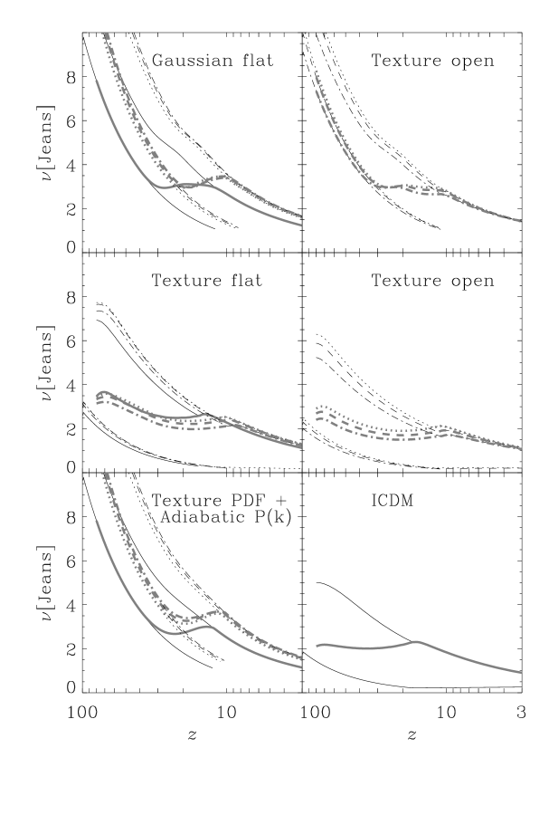
Figure 11:

Figure 12:

Figure 13:

Figure 14:

Figure 15:

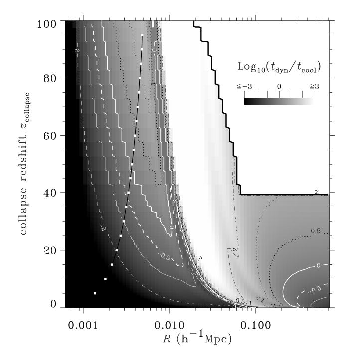
Figure 16:

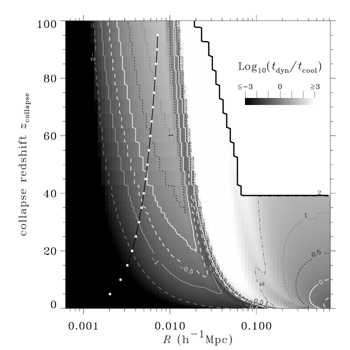
Figure 17:

References

- Abel (1998) Abel, T. 1998, http://zeus.ncsa.uiuc.edu/abel/PGas/codes.html
- Abel et al. (1998) Abel, T., Anninos, P., Zhang, Y., and Norman, M. L. 1997, New Astronomy, 2, 181
- Anninos et al. (1998) Anninos, P., Zhang, Y., Abel, T., and Norman, M. L. 1998, New Astronomy, 2, 209
- Bardeen et al. (1986) Bardeen, J. M., Bond, J. R., Kaiser, N., and Szalay, A. S. 1986, ApJ, 304, 15
- Binney (1977) Binney, J. J. 1977, ApJ, 215, 483
- Black (1981) Black, J. H. 1981, MNRAS, 197, 553
- Blain and Longair (1993) Blain, A. W. and Longair, M. S. 1993, MNRAS, 264, 509
- Bond et al. (1991) Bond, J. R., Cole, S., Efstathiou, G., and Kaiser, N. 1991, ApJ, 379, 440
- Cen (1992) Cen, R. 1992, ApJS, 78, 341
- Chiu, Ostriker, and Strauss (1997) Chiu, W., Ostriker, J. P., and Strauss, M. A. 1997, ApJ, 494, 479
- Ciardi et al. (1999) Ciardi, B., Ferrara, A., Governato, F., and Jenkins, A. 1999, preprint, astro-ph/9907189.
- Cole, Fisher, and Weinberg (1994) Cole, S., Fisher, K. B., and Weinberg, D. H. 1994, MNRAS, 267, 785
- Couchman and Rees (1986) Couchman, H. M. P. and Rees, M. J. 1986, MNRAS, 221, 53
- Efstathiou et al. (1988) Efstathiou, G., Frenk, C. S., White, S. D. M., and Davis, M. 1988, MNRAS, 235, 715
- Fixsen et al. (1997) Fixsen, D. J., Cheng, E. S., Gales, J. M., Mather, J. C., Shafer, R. A., and Wright, E. L. 1997, ApJ, 473, 576
- Giallongo et al. (1994) Giallongo, E., D’Odorico, S., Fontana, A., McMahon, H. G., Savaglio, S., Cristiani, S., Molaro, P., and Treverse, D. 1994, ApJ, 425, L1
- Gnedin (1996) Gnedin, N. Y. 1996, ApJ, 456, 1
- Gnedin and Ostriker (1997) Gnedin, N. Y. and Ostriker, J. P. 1997, ApJ, 486, 581
- Gooding et al. (1992) Gooding, A. K., Park, C., Spergel, D. N., Turok, N., and Gott, III, J. R. 1992, ApJ, 393, 42
- Janev et al. (1987) Janev, R. K., Langer, W. D., Evans, K. J., and Post, D. E. J. 1987, Elementary Processess in Hydrogen-Helium Plasmas, New York: Springer-Verlag
- Jenkins and Ostriker (1991) Jenkins, E. B. and Ostriker, J. P. 1991, ApJ, 276, 33
- Kaiser (1984) Kaiser, N. 1984, ApJ, 284, L9
- Kashlinsky and Rees (1983) Kashlinsky, A. and Rees, M. J. 1983, MNRAS, 205, 955
- Katz, Weinberg, and Hernquist (1996) Katz, N., Weinberg, D. H., and Hernquist, L. 1996, ApJS, 105, 1
- Kauffmann, Nusser, and Steinmetz (1997) Kauffmann, G., Nusser, A., and Steinmetz, M. 1997, MNRAS, 286, 795
- Lacey and Cole (1993) Lacey, C. G. and Cole, S. 1993, MNRAS, 262, 627
- Lacey and Cole (1994) Lacey, C. G. and Cole, S. 1994, MNRAS, 271, 676
- Lepp and Shull (1983) Lepp, S. and Shull, J. M. 1983, ApJ, 270, 578
- Mo and White (1996) Mo, H. J. and White, S. D. M. 1996, MNRAS, 282, 347
- Ostriker and Gnedin (1996) Ostriker, J. P. and Gnedin, N. Y. 1996, ApJ, 472, L63
- Park, Spergel, and Turok (1991) Park, C., Spergel, D. N., and Turok, N. 1991, ApJ, 372, L53
- Pearce et al. (1999) Pearce, F. R. et al. 1999, preprint, astro-ph/9905160.
- Peebles (1993) Peebles, P. J. E. 1993, Principles of Physical Cosmology, Princeton: Princeton University Press
- Peebles (1999a) Peebles, P. J. E. 1998a, ApJ, 510, 523
- Peebles (1999b) Peebles, P. J. E. 1998b, ApJ, 510, 531
- Pen and Spergel (1995) Pen, U. and Spergel, D. N. 1995, Phys. Rev. D, 49, 692
- Pen, Spergel, and Turok (1994) Pen, U., Spergel, D. N., and Turok, N. 1994, Phys. Rev. D, 51, 4099
- Press and Schechter (1974) Press, W. H. and Schechter, P. 1974, ApJ, 187, 425
- Press et al. (1992) Press, W. H., Teukolsky, S. A., Vetterling, W. T., and Flannery, B. P. 1992, Numerical Recipes in C, 2nd edition, Cambridge: Cambridge University Press
- Rauch et al. (1997) Rauch, M. et al. 1997, ApJ, 489, 7
- Rees and Ostriker (1977) Rees, M. J. and Ostriker, J. P. 1977, MNRAS, 179, 541
- Robinson and Baker (1999) Robinson, J. and Baker, J. E. 1999, preprint, astro-ph/9905098
- Robinson, Gawiser, and Silk (1998) Robinson, J., Gawiser, E., and Silk, J. 1998, preprint, astro-ph/9805181
- Sasaki (1994) Sasaki, S. 1994, PASJ, 46, 427
- Shapiro and Kang (1987) Shapiro, P. R. and Kang, H. 1987, ApJ, 318, 32
- Shapiro and Giroux (1987) Shapiro, P. R. and Giroux, M. L. 1987, ApJ, 321, L107
- Shapiro, Giroux, and Babul (1994) Shapiro, P. R., Giroux, M. L., and Babul, A. 1994, ApJ, 427, 25
- Silk (1977) Silk, J. 1977, ApJ, 211, 638
- Spitzer (1978) Spitzer, L., J. 1978, Physical Processes in the Interstellar Medium, New York: Wiley.
- Spitzer and Hart (1979) Spitzer, L., J. and Hart, M. H. 1979, ApJ, 442, 480
- Sugiyama (1995) Sugiyama, N. 1995, ApJS, 100, 281
- Tegmark et al. (1997) Tegmark, M., Silk, J., Rees, M. J., Blanchard, A., Abel, T., and Palla, F. 1997, ApJ, 474, 1
- Valageas and Silk (1999) Valageas, P. and Silk, J. 1999, å, in press
- Viana and Liddle (1996) Viana, P. T. P. and Liddle, A. R. 1996, MNRAS, 281, 323
- Zaldarriaga (1998) Zaldarriaga, M. 1998, PhD thesis, MIT