All sky mapping of the Cosmic Microwave Background at $8\hbox{${}^{\prime}$}$ angular resolution with a 0.1 K bolometer: simulations

Abstract

We present simulations of observations with the 143 GHz channel of the Planck High Frequency Instrument (HFI). These simulations are performed over the entire sky, using the true angular resolution of this channel: 8 arcmin FWHM, 3.5 arcmin per pixel. We show that with measured 0.1 K bolometer performances , the sensitivity needed on the Cosmic Microwave Background (CMB) survey is obtained using simple and robust data processing techniques, including a destriping algorithm.

Key words: 03.09.1 (Instrumentation: detectors), 03.13.2 (Methods: data analysis), 12.03.1 (cosmic microwave background)

1 Introduction

The ESA Planck mission, to be launched in 2007, will perform a quasi complete survey of the Cosmic Microwave Background (CMB) with an angular resolution reaching $5\hbox{${}^{\prime}$}$. It will use a 1.5 metre diametre off-axis telescope placed at the lagrangian L2 point, about 1.5 million kilometres from the Earth, in the antisolar direction. The focal plane includes two instruments, LFI and HFI, using respectively HEMTS and bolometer technologies. The frequency range is from 30 to 100 GHz for the LFI (beam sizes from $30\hbox{${}^{\prime}$}$ to $10\hbox{${}^{\prime}$}$), and from 100 to 857 GHz for the HFI ($11\hbox{${}^{\prime}$}$ to $5\hbox{${}^{\prime}$}$) . (for a detailed description see Bersanelli et al. [1994] and the Web pages at http://astro.estec.esa.nl/planck/). Planck will allow to grasp details on the last scattering surface which are more than ten times smaller than the size of the horizon at the epoch of recombination. The observed pattern will inform us on the statistics of the primordial seeds that have been generated in the very early universe, providing a unique observational test to fundamental physics. In addition, the maps will probe the Universe to an unprecedented distance, $z\simeq 1000$, allowing to derive the important cosmological parameters which determine its geometry (see e.g. Bond et al. [1997] and White et al. [1998]).

There are many observational difficulties to this challenge. Some are astrophysical (contamination by foregrounds) and others are instrumental (e.g. far sidelobe pickup and detector noises). The effects of the astrophysical foregrounds have been discussed in various papers and it has been demonstrated that the CMB can be recovered down to the level of the cosmic variance if adequate frequency bands are used (see e.g. Gispert and Bouchet [1996], or Linden-Vornle and Norgaard-Nielsen [1998]). The instrumental limitations seem to be a much more uncertain issue. The detector behaviour is one of the most critical instrumental issues. Janssen et al. [1996] investigated the problem of 1/f noise contamination for the PSI and FIRE proposals to NASA’s Medium-class Explorer program. Their study demonstrated that, given the performances of the detectors (bolometers and HEMTs), a simple scan by scan drift removal was enough to subtract most of the temporally correlated noise (e.g. 1/f noise) without any significant alteration of the CMB power spectrum. A more sophisticated method presented by Delabrouille ([1998]) uses the scans intersects redundancy to determine and subtract the low frequency useless signals. Except in very recent works (see the draft by Maino et al. [1999]), up to now, mostly for computational reasons, this destriping has been simulated at a very limited angular resolution (about 1 degree).

In this paper we present all sky simulations of CMB observations in the 143 GHz channel of the HFI instrument with a 0.1K bolometer. This channel is simulated with its true beam width, 8 arcmin full width at half maximum (FWHM), using sky maps with a pixel size of 3.5 arcmin. We show that a simple data processing (pixels binning) including a destriping algorithm, allows to efficiently eliminate the 1/f noise. The next section shows the measured performances of Planck prototype bolometers mounted on a 0.1 K open cycle ${}^{3}He/^{4}He$ dilution refrigerator. Section 3 deals with the simulations of all-sky Planck observations and map reconstruction. The results are discussed in section 4.

2 Performances of 0.1K bolometers

Prototype spiderweb bolometers with time constants suitable for Planck, e.g. a few milliseconds, have been integrated on a 0.1 K open cycle dilution refrigerator. The readout system uses a square-wave current control of the bolometer thermistor with capacitive load. This full digitally controled system is described in Gaertner et al. [1997]. It has been optimized to mimize power consumption, given the Planck needs. Those are: time frequency coverage from 0.01 to 200 Hz and sensitivity of order $3nV/Hz^{0.5}$ (corresponding to the typical Johnson noise of the bolometer thermistor, a few megohms). Fig. 1 shows the electrical noise performance of this system tested on a 300K resistor (a), and on a 0.1K Planck prototype bolometer (b). The measurement on the resistor demonstrates that the performance of the modulation control system plus amplifier chain fullfills the noise level requirement. The bolometer noise power spectrum has been obtained with an active temperature control of the 0.1 K plate. Volts have been calibrated against watts using the bolometer electrical response derived from the I(V) curve:

Fig. 1.: Measured noise performances on a 0.1 K prototype spiderweb bolometer (lower), and a pure resistor (upper). The 1/f noise on the bolometer is due to temperature unstabilities of the 0.1 K stage. The dashed line on the lower plot is the noise power spectrum used in the simulation, $f_{knee}=0.6Hz$ (see text).

$$\frac{dV}{dP}(volt/watt)=\frac{R-Z}{2RI}$$ (1)

where $Z=dV/dI$ is the dynamical impedance of the bolometer and $R=V/I$ is its resistance. The bolometer sensitivity in this system is of the order of $\,{\,10}^{-17}W/Hz^{-0.5}$ for all frequencies larger than 1 Hz. The excess noise at lower frequencies has been attributed to residual temperature fluctuations of the 0.1 K system. Its thermal origin is demonstrated by the correlation with the bolometer response: this noise is always at the same level in terms of ”Watts” for different system temperatures, thus bolometer responses, whereas the high frequency plateau in the noise spectrum has a constant level in terms of ”volts”, whatever is the bolometer response. Most of the 0.1 K temperature fluctuations are due to instabilities in the flow of the cooling fluids. Current studies of the 0.1K refrigerator system aim at reducing this problem together with improving the active temperature control of the bolometer plate. However, our simulations in section 3 show that this noise level is acceptable and already allows to measure the CMB signal with the required accuracy.

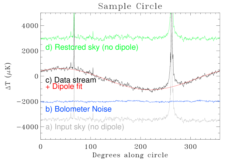
Fig. 2.: A sample simulated circle showing the co-added signal from a single 143 GHz bolometer between two satellite pointings.

3 All sky simulations

3.1 Simulating the data stream

We have simulated 12 months of the Planck mission with the following observing strategy: the satellite spin rate is $S=1$ rpm, with the spin axis following the antisolar direction. The beam scans the sky at an angular distance of 85 degrees from the spin axis. Re-pointing of the spin axis to follow the antisolar direction is performed with a step of 2.5 arcmin (i.e. a period $T\simeq 61minutes$). The spin axis follows a sinusoïdal trajectory along the ecliptic with full amplitude $\Delta\delta=\pm 10$ degrees, so that the polar caps are not left unobserved. A duration of 12 months is the minimum which allows to observe twice at 6 months interval almost all directions of the sky, thus providing redundancy.

In this simulation, the observed sky is the sum of the CMB, including the COBE-DMR determination of the CMB dipole (Lineweaver et al. [1996]), and the Galaxy extrapolated from the composite 100 $\,{\mu m}$ IRAS-COBE/DIRBE all sky dataset (Schlegel et al. [1998]). This extrapolation assumes a dust spectrum typical of high latitude cirrus clouds, $T_{d}=17K,n_{d}=2$ (Boulanger et al. [1996]). The CMB sky is obtained from a standard Cold Dark Matter model: $\Omega_{tot}=1$, $\Omega_{b}=0.05$, $\Omega_{\Lambda}=0$, and $\,{H_{0}}=50km/s/Mpc$. We compute the $\,{C_{l}}$ power spectrum with CMBFAST (Seljak et al. [1996]) and the map is generated in a Healpix-type all-sky pixellisation with a pixel size of 3.5 arcmin (Górski [1998], see the web pages at http://www.tac.dk/~healpix). Since our simulations will be limited to the frequencies of the HFI instrument, $\nu\geq 100GHz$, we do not include the galactic synchrotron and free-free emissions. The COBE/DMR data analysis from Kogut et al. ([1996]) has shown that both are smaller than the dust at such frequencies, the former being highly correlated with the dust. The radio point sources are not included either, and they are supposed to be extracted on a scan by scan analysis. The instrumental noise is added after pickup of the sky signal on a scan by scan basis. The noise power spectrum follows the characteristics of our 0.1 K bolometer system, and is the sum of a white noise and 1/f low frequency noise:

$$N=N_{\infty}*(1+f_{knee}/f)$$ (2)

With typical values being, $N_{\infty}=52\mu K/Hz^{0.5}$ (physical temperature) for the millimeter channels, and $f_{knee}=0.6Hz$.

In order to spare computer time, only one scan (called circle in the following) is simulated between two satellite re-pointings. The noise level is correspondingly reduced by factor $(T/S)^{0.5}=7.8$, assuming that all the scans are coadded into a single circle and that the noise is not correlated from one scan to the other. This is not strictly correct given the frequency aliasing produced by the co-addition (see Janssen et al. [1996]). However we have checked that this is correct within the statistics of the noise. Fig. 3 demonstrates this: we have plotted here the power spectrum of the circle obtained by the averaging of 64 scans (one hour of observing time) and compare it to the average power spectrum of a single scan (i.e. Equ. 2) divided by the square root of the number of scans coadded. The data sampling along the scan direction is equal to the depointing step: 2.5 arcmin. The time frequency domain is thus sampled from 0.016 Hz (spin frequency) to 144 Hz (sampling rate).

Fig. 3.: The power spectrum of a simulated circle obtained by averaging 64 scans (dots) is compared to the average power spectrum of a single scan (dashed line) and the average scan power spectrum divided by $\sqrt{6}4$ (thick dashed line). For FFT efficiency 64 was used instead of 60, the exact number of scans per circle.

3.2 Data processing and destriping algorithm

To construct the simulated sky maps, the data from the circles are simply coadded within the pixels of the map. As usual with bolometric devices, the absolute level of the measured power is unknown.

At zero order, the level of each circle is adjusted by subtraction of a constant so that the measured signal fits a cosecant law (galactic dust) plus dipole emission:

$$M_{ik}=r_{k}(Dipole_{ik}+\frac{g_{k}}{sin(bII_{i})}+C^{0}_{k})$$ (3)

k is the circle index, and i the data index along the circle. The free parameters are: $g_{k}$ the level of the galactic emission for this circle, and $C^{0}_{k}$ the constant to be subtracted. The detector response, $r_{k}$, is supposed to be fixed and known from calibration procedures. Portions of the circle with a strong signal ( $>6mK$ or $|lII|<10^{\circ}$ ) or a strong gradient (point sources) are excluded from the fit. The cosecant law is introduced in the fit to avoid subtraction of the average galactic signal, which is positive. The calibrated data projected on the final survey map is then:

$$D_{ik}=M_{ik}/r_{k}-C^{0}_{k}-Dipole_{ik}$$ (4)

Fig. 2 shows a sample simulated circle (addition of about 60 scans) for one bolometer of the frequency band centered at 143 GHz. The dipole and the Galaxy are the dominating signals. On this circle the Galactic plane is intercepted at Galactic longitudes of about 18 and 195 degrees. The primary fluctuations of the CMB are clearly visible on the measured signal for this single bolometer measurement.

This coarse evaluation of the offset of each circle is not sufficient to obtain the high quality maps required for the Planck mission. We further destripe the data using an algorithm derived from Delabrouille ([1998]) which uses the scan intercepts. We actually adjust the constants $C^{1}_{k}$ to subtract to each circle $k$ by minimising the spread between the measurements contributing to the same sky pixel. This is done globally for all the sky pixels using for each pixel a weight wich is proportional to the number of circles contributing to this pixel. The quantity to be minimised thus reads:

$$J=\sum_{ipix\,\in\,Sky}\left[\frac{\sum_{ik\,\in\,ipix}(D_{ik}-C^{1}_{k})^{2}}{n(ipix)}-\left(\frac{\sum_{ik\,\in\,ipix}(D_{ik}-C^{1}_{k})}{n(ipix)}\right)^{2}\right]$$ (5)

$ik\,\in\,ipix$ means that the sum is over all measurements from circle k and index i contributing to pixel ipix.

$n(ipix)$ is the total number of measurements contributing to a given sky pixel.

We find the minimum of $J$ using a maximum gradient iterative algorithm. At each iteration the optimal step length in the direction of the gradient can be computed exactly because $J$ is a quadratic form. The gradient reads:

$$\frac{\partial J}{\partial C^{1}_{k}}=2\sum_{i\,\in\,k}\left[\frac{\sum_{i^{\prime}k^{\prime}\,\in\,ipix(ik)}(D_{i^{\prime}k^{\prime}}-C^{1}_{k^{\prime}})}{n(ipix(ik))}-(D_{ik}-C^{1}_{k})\right]/n(ipix(ik))$$ (6)

$i\,\in\,k$ means that the sum is over all data points from circle k, and $i^{\prime}k^{\prime}\,\in\,ipix(ik)$ means that the sum is over all measurements falling on the same sky pixel ipix(ik) as measurement ik.

The optimal iterative step is:

$$\Delta C^{1}_{k}=\alpha\frac{\partial J}{\partial C^{1}_{k}}$$ (7)

with

$$\alpha=\frac{\sum_{ipix\,\in\,Sky}\left[\frac{\sum_{ik\,\in\,ipix}\frac{\partial J}{\partial C^{1}_{k}}}{n(ipix)}\frac{\sum_{ik\,\in\,ipix}(D_{ik}-C^{1}_{k})}{n(ipix)}-\frac{\sum_{ik\,\in\,ipix}\frac{\partial J}{\partial C^{1}_{k}}(D_{ik}-C^{1}_{k})}{n(ipix)}\right]}{\sum_{ipix\,\in\,Sky}\left[\left(\frac{\sum_{ik\,\in\,ipix}\frac{\partial J}{\partial C^{1}_{k}}}{n(ipix)}\right)^{2}-\frac{\sum_{ik\,\in\,ipix}\frac{\partial J}{\partial C^{1}_{k}}^{2}}{n(ipix)}\right]}$$ (8)

Figure 4 shows the convergence of our iterative destriping method which evaluates the best constants to subtract to each circle. We plot in this Figure the average over the whole sky of the rms spread of the data within a pixel (i.e. $sqrt(J/npix)$). This is shown for two different starting conditions: i) the stars are obtained with a simplistic starting condition which consists in forcing the average signal of each circle to be nul, ii) the diamonds are obtained starting from circles where the constant subtracted has been set using (3): a fit which includes the CMB dipole and a cosecant galactic law. This second method is very efficient and a relative precision better than 1.e-4 is obtained within five or six iterations of the starting point. The value of 1.e-4 for the relative precision on the final average rms is the criterium that we have fixed to end the destriping iterations. The triangles show the result for a pure white bolometer noise (no 1/f noise). The comparison of the final rms values for both cases shows an excess of about 15% for the 1/f noise with respect to the white noise. This is to be compared to the noise excess induced by the 1/f tail : 10% on the rms for a knee frequency of 0.6 Hz if we take into account only the frequencies higher than the spin rate (0.016 Hz). In fact the noise at frequencies smaller than the spin rate has not been fully washed out since we only subtract a constant level to each circle. A Wierner filtering in the frequency domain would be optimum, but this would alter the astrophysical signal.

Fig. 4.: Convergence of the iterative maximum gradient algorithm used to destripe the data. The upper plot shows the average rms spread of the data points falling into a single pixel as a function of the iteration step. The stars show the convergence from a starting point where each circle has been set to a null average. The diamonds are obtained with a starting point where the constant subtracted to each circle is evaluated in a fit which includes the CMB dipole plus a cosecant law (see equ. 4). The triangles are obtained for a pure white bolometer noise. The lower plot shows the relative difference between the current and final rms value.

Our simulations are performed on a Pentium III 500 MHz processor using the IDL environment. The data are first generated for the full mission and stored in a file with the corresponding sky pixel indexes. This needs about 30 minutes of computer time. Then the iterations are performed, which needs about 20 minutes each, so that the time for a full simulation with destriping is less than 2 hours.

The computation of the spherical harmonics power spectrum from the simulted map is about the same duration, using the fast code implemented with the Healpix package (Hivon and Górski [1998]). The signal at galactic latitudes bellow 30 degrees is set to zero for the $\,{C_{l}}$ power spectrum estimation. This implies some aliasing of the galactic component for the low l values (see below).

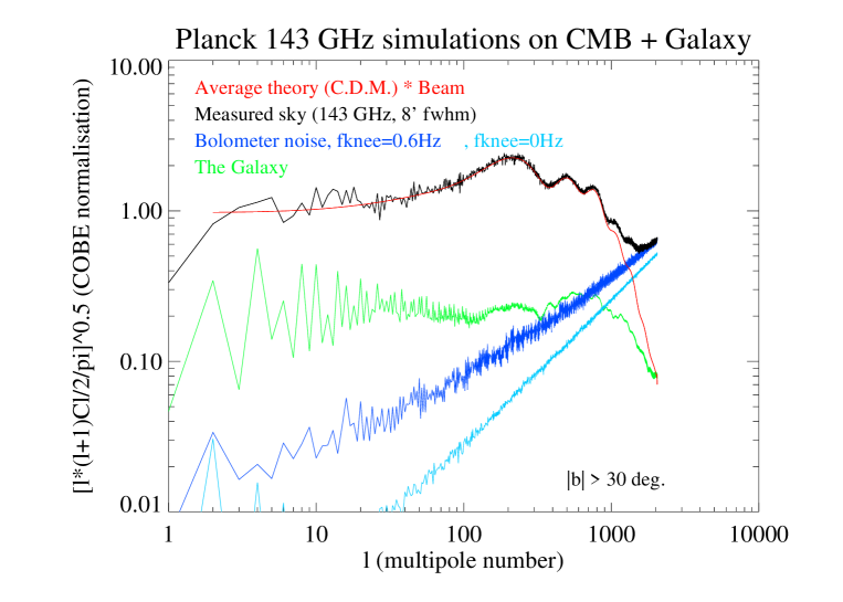
Fig. 5.: Black: $\,{C_{l}}$ transform of the simulated reconstructed sky at 143 GHz for 6 bolometers, 12 months (galactic latitudes bellow 30 degrees have been set to zero). Red: average theory from which the CMB sky was generated (convolved by the instrumental beam: 8 arcmin FWHM gaussian). Green: contribution from the galactic dust. Blue: contribution from the bolometer noise with 1/f noise (dark) and for pure white noise (light).

4 Results and conclusion

Fig. 7 shows the allsky average map for six bolometers at 143 GHz. It has been obtained by averaging six simulations with independent noise realisations. This is certainly a simplistic assumption since one can expect the bolometer noises to be correlated. However, such correlated noises will be monitored by thermometers and blind bolometers. The average signal-to-noise ratio on each 3.5 arcmin pixel of this map is about 6 at high galactic latitudes, where the CMB dominates, the rms signal and noise being respectively $110$ and $22\mu K$. The variance of the reconstructed map for a single bolometer has been computed using a Monte-Carlo method which repeats the simulation for different noise seeds. Fig. 8 and 9 show respectively the variance for the non-destriped and destriped map estimated from 28 simulations. The gain induced by the use of the destriping is clearly visible.

The noise due to the data processing has been estimated in a simulation performed with no instrumental noise. The destriping has been iterated 6 times, which is the average number of iterations needed to reach the convergence criterium in the case where the instrumental noise is included. The map obtained by difference from this simulation and the input sky is shown in Fig. 10. The level of this difference is always below a few $\mu K$, demonstrating that the data processing noise is negligible compared to the instrumental noise. Moreover, its level can be lowered by several orders of magnitude by simply increasing the number of iterations in the destriping algorithm.

We have also computed the noise correlation of a particuliar pixel with all other sky pixels. The pixel is located at galactic coordinates (LII, BII) = ($45\,{{}^{{o}}}$, $28\,{{}^{{o}}}$). The correlation coefficient of this pixel with others is shown for the sky region arround that pixel in Fig. 11 a and b (respectively non-destriped and destriped). The number of iterations for this estimation has been set to 128. It needs to be much higher than for the auto-covariance since the average value is in general close to zero. The correlation of the central pixel with its neighbours is, as expected, maximum along the circles intercepting this pixel. It is clearly improved with the iterative destriping. The spread in the values of the estimated correlation for the other pixels is actually dominated by the error of the Monte-Carlo method : about $5\,{\,10}^{-10}K^{2}$ ($rms^{2}$) for 128 iterations and a rms noise in this part of the sky of $70\,{\,10}^{-6}$ K.

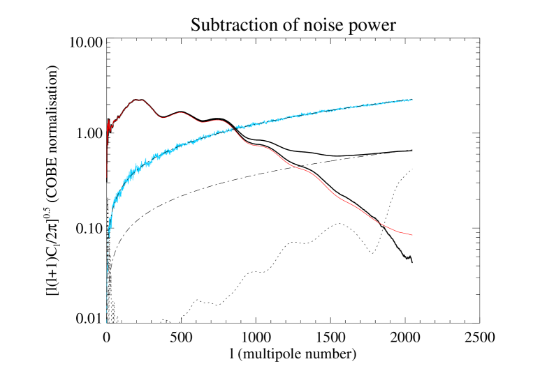
Fig. 6.: Recovered smoothed $\,{C_{l}}$ for the 12 months simulation (thick black) compared to the original $\,{C_{l}}$ (red) at 143 GHz. Blue: pure noise from a 2 bolometer difference fitted by a log-log 3rd order polynomial (black dashed) and adjusted to the measured $\,{C_{l}}$ at high l’s (black dot-dashed). Black dots : relative error on the recovered $\,{C_{l}}$.

The $C_{l}$ power spectra of the reconstructed sky and the various components are plotted in Figure 5. We did not try here to correct for the beam of the instrument. Our simulated beam is a gaussian of 8 arcmin FWHM. This could be removed in $\,{C_{l}}$ space by division of the measured spectrum by the $\,{C_{l}}$ transform of the beam. However, the true beam will not be symmetrical (due to the off-axis telescope and the electrical signal filtering in the scanning direction) so that such a method will provide only a first order approximation. One will actually need more sophisticated inversion methods which are out of the scope of this paper.

The bolometer noise dominates the power-spectrum at high multipole numbers. Its estimation and subtraction will be a critical step for the recovery of the astrophysical sky power-spectrum for these multipole numbers. The shape of the noise power spectrum can practically be estimated from a pure noise map obtained by difference from 2 bolometers. Its level can then be adjusted to the measured (sky+noise) power-spectrum at high multipole numbers and subtracted. Fig. 6 compares the recovered power spectrum to the original one. The noise power spectrum from a 2 bolometer difference has been fitted by a 3rd order polynomial in log-log scale and then quadratically subtracted to the sky measured power-spectrum, after adjustment on high multipole numbers, $l>1950$. In this Figure the final and original $\,{C_{l}}$’s have been smoothed by a square window of constant logarithmic width (dl/l = 0.1), thus reducing the fluctuations due to the cosmic variance. The relative error on the recovered $\,{C_{l}}$ is also shown in Fig. 6. Its level is below 1 % for $l<500$ , and rises from 1 % to 10 % for $500<l<1950$.

The galactic emission, which has not been subtracted in our data processing, dominates the errors at high multipole numbers. Informations from the Planck higher frequency channels will be used to subtract this component. The accuracy of this subtraction will be limited by the uncertainty in the values of the dust spectral index and temperature deduced from the submillimeter channels. A conservative estimate of the residual galactic signal can be obtained if we assume that the relative error on the estimation of the galactic signal is of the order of 10 %. With this hypothesis the galactic residual will never be higher than 3 % of the CMB up to the higher l values ( $l<2048$, see Fig. 6).

The simulations presented in this paper address a limited number of points, both with regard to the astrophysical sky (we include only the CMB and the galactic dust which are dominant at 143 GHz) and to the instrument (only one frequency channel instead of the 9 channels of the two Planck focal plane instruments). As mentioned in Sect. 1 there will be systematic signals produced by temperature variations in the payload. The galactic signal picked up in the far side lobes of the telescope will be significant, even at high galactic latitudes. A proper analysis of the data, with optimal rejection of the systematics and noise sources for reconstructing the sky maps, will have to involve a global strategy making use of all frequency channels. Our result, however, show that even a single channel analysis at 143 GHz, which assumes noise performances measured on a prototype bolometer mounted on a 0.1 K open cycle dilution refrigerator, produces satisfactory results.

Acknowledgements. Map projections routines and power spectrum calculations were performed with the Healpix package written by Górski, Hivon and Wandelt (http://www.tac.dk/healpix). KG and EH were funded by the Dansk Grundforskningsfond through its funding for TAC. E.H. and A.L. were supported in part by NASA Grant NAG5-6573.

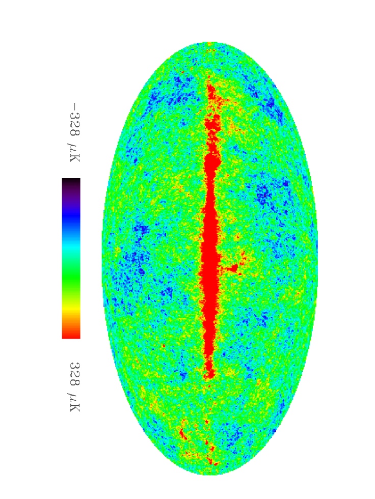
Fig. 7.: Simulated allsky reconstructed map at 143 GHz for the 12 months of the Planck missions (average of 6 bolometers).

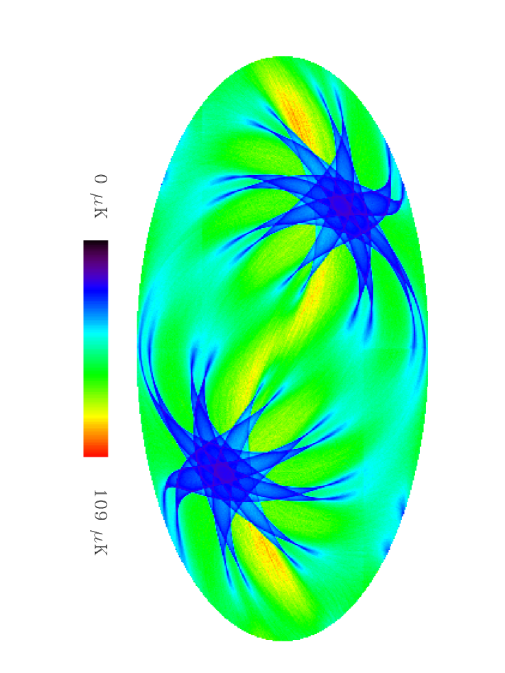
Fig. 8.: Variance map at 143 GHz for 12 months of the Planck mission: no destriping included.

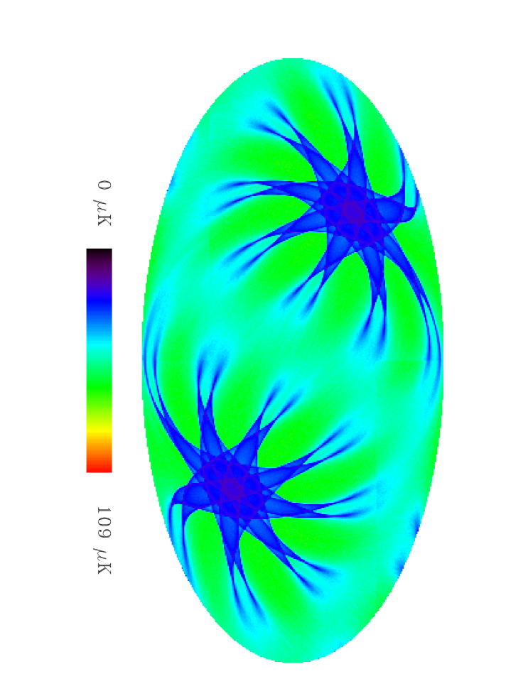
Fig. 9.: Variance map at 143 GHz for 12 months of the Planck mission: destriping included.

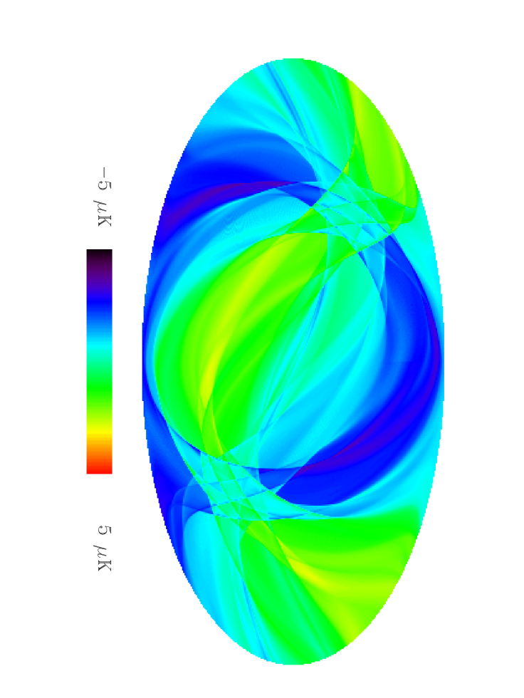
Fig. 10.: Map of the residual striping after 6 iterations of the maximum gradient algorithm. This is the difference between the input sky and the sky recovered after a simulation with no instrumental noise.

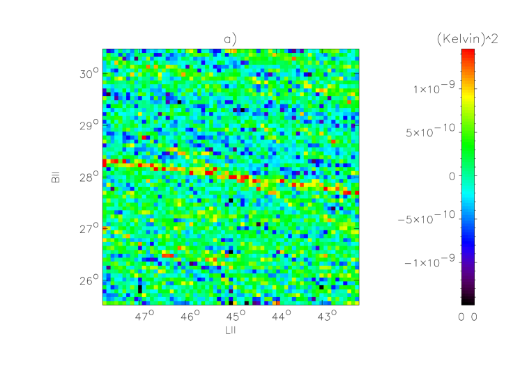
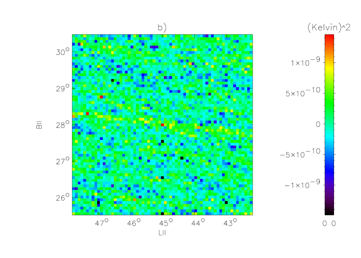
Fig. 11.: Estimated covariance map for a pixel at $(LII,BII)=(45\deg,28\deg)$ with its neighbour pixels : a) no destriping included, b) destriping included.

References

- 1994 Bersanelli, M., Bouchet, F., Efstathiou, G., Griffin, M., Lamarre, J.M., Mandolesi, R., Nogaard-Nielsen, H., Pace, O., Polny, J., Puget, J.L., Tauber, J., Vittorio, N. and Volont , S., 1996, COBRAS/SAMBA Phase A report.
- 1997 Bond, J. R., Efstathiou, G., and Tegmark, M., 1997, MNRAS 291, L33
- 1996 Boulanger, F., Abergel, A., Bernard, J.P., Burton, W.B., Désert, F.X., Hartmann, D. Lagache, G., and Puget, J.L., 1996, ApJ 312, 256
- 1998 Delabrouille, J., 1998, PhD Thesis
- 1998 Delabrouille, J., 1998, A&A Supl. 127, 555
- 1997 Gaertner, S., Benoit, A., Lamarre, J.M., Giard, M., Bret, J.L., Chabaud, J.P., Désert, F.X., Faure, J.P., Jegoudez, G., Lande, J., Leblanc, J., Lepeltier, J.P., Narbonne, J., Piat, M., Pons, R., Serra, G., Simiand, G., 1997, A&A Sup. 126, 151
- 1996 Gispert, R., and Bouchet, F. R., 1996, in Proc. of the 16th Moriond Astrophysics meeting, Les Arcs, France, p 503, 509.
- 1998 Górski, K., 1998, in preparation
- 1998 Hivon, E., and Górski, K., 1998, in preparation
- 1996 Kogut, A., Banday, A. J., Bennett, C. L., Górski, K. M., Hinshaw, G., and Reach, W. T. 1996, ApJ, 460, 1
- 1998 Linden-Vornle, M.J.D., and Norgaard-Nielsen, H.U., 1998, A&A Supl. 128, 377
- 1996 Janssen M., Scott, D., White, M., Seiffert, M.D., Lawrence, C.R., Górski, K.G., Dragovan, M., Gaier, T., Ganga, K., Gulkis, S., Lange, A.E., Levin, S.M., Lubin, P.M., Meinhold, P., Readhead, A.C.S., Richards, P., and Ruhl, J., 1996, astro-ph/9602009
- 1996 Lineweaver, C.H., Tenorio, L., Smoot, G.F., Keegstra, P., Banday, A.J., and Lubin, P., 1996, ApJ 470, 38
- 1999 Maino D., Burgarina, C., Maltoni, M., Wandelt, B.D., Górski, K.M., Malaspina, M., Bersanelli, M., Mandolesi, N., Banday, A.J., and Hivon, E., 1999, astro-ph/9906010.
- 1998 Schlegel, D.J., Finkbeiner, D.P., and Davis, M., 1998, ApJ 500, 525
- 1996 Seljak, U., and Zaldarriaga, M., 1996, ApJ 469, 437
- 1998 White M., 1998, astro-ph 9802295