The BL Lac Object Mkn 501 was in a state of high activity in the TeV range in 1997. During this time Mkn 501 was observed by all Cherenkov-Telescopes of the HEGRA-Collaboration. Part of the data were also taken during moonshine thus providing a nearly continuous coverage for this object in the TeV-range. We have carried out a QPO analysis and found evidence for a 23 day periodicity. We applied the same analysis on the ’data by dwell’ x-ray lightcurve from the RXTE/ASM database and found also evidence for the 23 day periodicity. The combined probability was ${\cal P}=2.8\,e$–$\,04$.

1 Introduction

The nearby AGN Mkn 501 ($z=0.034$) of the BL-Lac class is known to be one of the few TeV $\gamma$-ray (shortcut $\gamma$) sources. The source has been discovered in 1995 by the Whipple collaboration, Quinn et al. 1996, at a flux level equivalent to a few % of that of the Crab nebula and has been confirmed 1996 by the HEGRA collaboration, Bradbury et al. 1997.

Early in 1997 a large increase in the TeV $\gamma$-flux has been observed by at least 7 groups, see Protheroe 1997 for an overview. Observations covered the time from February until October. The flux was highly variable with a mean value of around 3 times and flares up to 10 times of that of the Crab.

Since 1996 Mkn 501 has been monitored in the 2-12 (10) keV X-ray band by the all sky monitor (ASM) of RXTE (Remillard 1997). The data are available as public domain (RXTE 1999) and presented either on rates per few hours or smoothed. The Mkn 501 X-ray data coverage is nearly continuous (with small gaps) and shows also a significant increase until mid 1997 and then a falling tendency. Again, significant fluctuations are observed, but much less dramatic compared to the TeV flux variation.

Already at the XXV ICRC, Durban, two groups (TA and HEGRA) reported about indications for periodicity in the TeV lightcurve, although no full analysis has been carried out. One of the problems was the interruption of the observations during the periods of moonshine. In the following the procedure and results of a QPO analysis to both the TeV and X-ray lightcurve will be presented.

2 The data

The TeV data were recorded with the 6 air Cherenkov telescopes of the HEGRA experiment located on the canary island La Palma. Four telescopes formed a stereo system (SCT) providing high statistics results from 110 hours of observation time. Less precise data were taken with the two standalone CTs. The latter instrument’s data correspond to 300 hours observation, in part overlapping with the SCT data. A sizable fraction of the data recorded with one of the standalone telescopes, CT1, was taken during moonshine, thus providing flux measurements when no other telescope was operational, see Aharonian et al. 1999a, Aharonian et al. 1999b, Kranich et al. 1999.

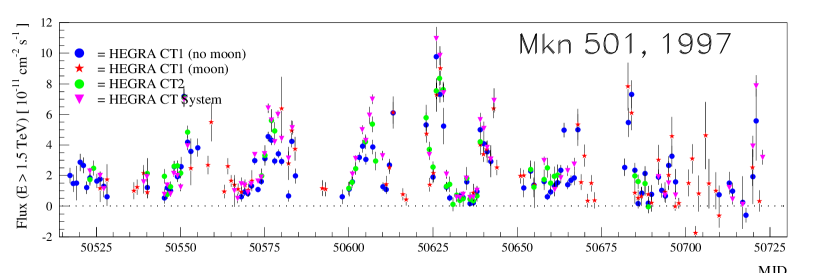
Figure 1: Lightcurve above 1.5 TeV energy; also shown is the X-ray lightcurve between 2 to 10 keV from RXTE-ASM. The one day averaged RXTE data are shown for clarity.

The used lightcurve above 1.5 TeV energy is shown in Fig. 1. Typical observation duration during summer 1997 was 3-4 hours/night whenever atmospheric conditions were acceptable. Fig. 1 also shows the X-ray lightcurve between 2 to 10 keV from RXTE-ASM. For clarity the smoothed data are shown while in the subsequent analysis the unsmoothed data ($\sim 3000$ data points) were used.

For the analysis the data between MJD 50545 and MJD 50661 were used. As starting date we took the onset of the high state while the second limit was taken where the X-ray curve was interrupted for some time. Additional reason to end the analysis at MJD 50661 was the fact that the later TeV data were taken only at large zenith angles and rather short observation times per day. Also the source seemed to return to a lower state.

3 The periodicity analysis

As mentioned in the introduction and visible in Fig. 1 the TeV lightcurve shows indications of a periodic modulation. In order to test for a QPO structure we used the formalism developed by Lomb and Scargle (Lomb 1976, Scargle 1982) which is able to derive power spectra from unevenly sampled data. The Lomb normalized periodogram (nP) is a modification of the classical Periodogram (defined within the formalism of discrete Fourier transformations) and gives the spectral power as a function of angular frequency $\omega\equiv 2\pi f$. The nP is defined as:

$$P_{N}\left(\,\omega\,\right)={1\over 2\,\sigma^{2}}\left\lgroup{\left[\sum_{j}(h_{j}-\overline{h})\cos\,\omega\left(t_{j}-\tau\right)\right]^{2}\over\sum_{j}\cos^{2}\,\omega\left(t_{j}-\tau\right)}+{\left[\sum_{j}(h_{j}-\overline{h})\sin\,\omega\left(t_{j}-\tau\right)\right]^{2}\over\sum_{j}\sin^{2}\,\omega\left(t_{j}-\tau\right)}\right\rgroup\$$ (1)

with $\tau$ defined by the equation:

$$\tan\,\left(2\,\omega\,\tau\,\right)=\Bigl{(}\,\sum_{j}\sin\,2\,\omega\,t_{j}\,\Bigr{)}\ /\ \Bigl{(}\,\sum_{j}\cos\,2\,\omega\,t_{j}\,\Bigr{)}$$ (2)

The $h_{j}$ are the individual flux values measured at time $t_{j}$, and the sums extend over all $N$ data points. $\overline{h}$ is the mean value of the $h_{j}$.
This definition of $\tau$ makes $P_{N}\left(\,\omega\,\right)$ completely independent of a constant time shift of the data. It can be shown (Scargle 1982) that the normalization on the variance forces $P_{N}\left(\,\omega\,\right)$ to have an exponential probability distribution if the data values are independent Gaussian random values:

$${\cal P}\left(\,P_{N}\left(\,\omega\,\right)>z\,\right)\ \equiv\ \exp\,(-z)\ .$$ (3)

[1,r,, Power spectra for TeV (solid line) and x-ray data (dashed line).] The results from the analysis, carried out independently for the TeV and X-ray data set, are shown in Fig. 3. Both, the TeV and X-ray data show a significant peak at a frequency of $0.044\,d^{-1}$ which corresponds to a 23 day period. The 2nd harmonic of this period is visible in the X-ray data but not in the TeV data. Note that the high power value in the X-ray data at $f=1\,/\,T=0.0088\,d^{-1}$ corresponds to the overall behavior of the average count-rate during 1997 (increasing/decreasing count rates before/after MJD $\sim$ 50625).
From the power value for the 23 days period one can calculate the corresponding probability against the null hypothesis of independent Gaussian random noise. But since it is known that BL Lac objects show the phenomenon of flaring it is more meaningful to test against the null hypothesis of independent, random distributed flares (so-called shot noise model, see deJager 1999 and reference therein). In order to state probabilities within this framework it is necessary to renormalize nP. This can be done by calculating the mean Fourier power from the shot noise model. If one assumes flares of Gaussian shape with standard deviation $\sigma$ the mean Fourier power becomes:

$$\left<\,P_{f}\left(\,\omega\,\right)\,\right>=A\cdot\exp\,\left(\,-\omega^{2}\,\sigma^{2}\right)$$ (4)

Here $A\,\propto\,\overline{a^{2}}$ which is the mean squared amplitude of the flares. A maximum likelihood analysis of the derived power spectra of Fig. 3, but excluding the 23 day period and the first frequency $f=1\,/\,T$, gives the parameters $A=3.8$, $\sigma=0.41\,{\rm d}$ (TeV range) and $A=3.8$, $\sigma=0.35\,{\rm d}$ (X-ray range) (deJager 1999). The final Fourier power is then calculated as:

$$P\left(\,\omega\,\right)=P_{N}\left(\,\omega\,\right)/\left<\,P_{f}\left(\,\omega\,\right)\,\right>\,.$$ (5)

The distribution of $P\left(\,\omega\,\right)$ is shown in Fig. 3. The power values now follow the same $\exp\,\left(\,-z\,\right)$ distribution as in the case of independent Gaussian random noise (Equ. 3). Again the 23 day period points have big, but less significant deviations from this distribution.

Figure 2: Number of frequencies with a given (renormalized) power vs. power for the TeV (black squares) and X-ray data (open circles). Points without errors consist of one single frequency.

Figure 3: The combined power spectrum (X-ray and TeV data) using proper normalization (see text). The probability of the 23 day period, after multiplication with the number of trials, corresponds to 3.5 $\sigma$ .

The final significance for the 23 day period is derived from the power spectrum of the combined X-ray and TeV data. Here we use the fact that if ${\cal P}\equiv\exp\,\left(\,-z\,\right)$, for each single frequency

$$\chi^{2}\,\left(\,4\,\right)=-2\,\ln\,\left(\,\exp\,\left(\,-z_{\gamma}\,\right)\,\right)-2\,\ln\,\left(\,\exp\,\left(\,-z_{\hbox{x-ray}}\,\right)\,\right)=2\cdot(z_{\gamma}+z_{\hbox{x-ray}})$$ (6)

is chi-square distributed with 4 degrees of freedom. The resulting $\chi^{2}$ values together with the corresponding probability are shown in Fig. 3. For the 23 day period a probability ${\cal P}=4.9\,e$–$\,06$ corresponding to $4.4\,\sigma$ is derived, which reduces to ${\cal P}=2.8\,e$–$\,04$ or $3.5\,\sigma$ after taking all 58 independent trial frequencies (between 1/T and 0.5 per day) into account.

4 Results and Conclusions

The power spectrum shows a significant peak at 23 days in both the TeV and X-ray data samples. This result is in accordance with the significant correlation of 0.64 which has been observed between the TeV and X-ray data (Aharonian 1999b). Using the framework of the shot noise model the combined significance becomes 3.5 $\sigma$. In order to avoid/reduce aliasing effects, introduced by the data gaps during the moon period in the TeV range, moon observations have proven to be of great importance.

References

Aharonian, F.A., et al., 1999a, A&A 342, 69
Aharonian, F.A., et al., 1999b, A&A accepted, see also astro-ph/9901248
Bradbury, S.M., et al., 1997, A&A 320, L5
de Jager, O.C., Kranich, D., Lorenz, E. & Kestel, M., 1999, these proceedings
Kranich, D., et al., 1999, Astroparticle Physics accepted, see also
astro-ph/9901330
Lomb, N.R., 1976, Astrophysics and Space Science, 39, 447-462
Protheroe, R.J., et al., 1997, Proc. 25th ICRC, Durban, Vol. 8, 317
Quinn, J., et al., 1996, ApJ 456, L83
Remillard, R.A. & Levine, M.L., 1997, Proc. All Sky X-Ray Observations in
the Next Decade,
see also astro-ph/9707338
RXTE, 1999, ’ASM/RXTE quick-look results’, http://space.mit.edu/XTE/asmlc/ASM.html
Scargle, J.D., 1982, ApJ 263, 835