email: soeren@astro.ku.dk
Young massive star clusters in nearby galaxies ††thanks: Based on observations made with the Nordic Optical Telescope, operated on the island of La Palma jointly by Denmark, Finland, Iceland, Norway, and Sweden, in the Spanish Observatorio del Roque de los Muchachos of the Instituto de Astrofisica de Canarias, and with the Danish 1.5-m telescope at ESO, La Silla, Chile.
Abstract
111Table 4 is also available in electronic form at the CDS via http://cdsweb.u-strasbg.fr/Abstract.htmlA detailed description is given of the data analysis leading to the discovery of young massive star clusters (YMCs) in a sample of 21 nearby galaxies. A new useful tool, ishape, for the derivation of intrinsic shape parameters of compact objects is presented, and some test results are shown. Completeness tests for the cluster samples are discussed, and ishape is used to estimate cluster sizes. Half-light radii of 0 - 20 pc are derived for clusters in 2 of the most cluster-rich galaxies, NGC 1313 and NGC 5236, which is within the range spanned by globular clusters in the Milky Way and by YMCs in the LMC and some starburst galaxies. Photometric data for all clusters, along with positions and estimated half-light radii, are tabulated.
Key Words.:
Galaxies: individual – photometry – spiral – star clusters. Techniques: image processing.1 Introduction
This paper is the second in a series describing the observations of “young massive star clusters” (YMCs) in a number of nearby spiral and irregular galaxies. A general outline of the project was given by Larsen & Richtler (lr1999 (1999), Paper1), and some first results were presented there. In this paper the data reductions are discussed in more detail, with special emphasis on two software tools developed as part of the project, which may be of general use to the astronomical community. These tools are mksynth, a programme which generates synthetic images with realistic noise characteristics, and ishape which derives intrinsic shape parameters for compact objects in a digital image by convolving an analytic model profile with the PSF and matching the result to the observed profile.
By YMCs we mean objects of the same type as e.g. the cluster NGC 1866 in the Large Magellanic Cloud (Fischer et al. fischer1992 (1992)). They are characterised by being similar (with respect to mass and morphology) to globular clusters seen in the Milky Way, but of much lower ages - in fact, the lower age limit of the clusters in our sample is set only by the fact that we avoid objects located within HII regions.
The paper is organised as follows: The observations are described in Sect. 2, and Sect. 3 is a discussion of the basic data reduction procedure including the standard calibrations. In Sect. 4 the tools mksynth and ishape are introduced, and Sect. 5 gives a discussion of the completeness corrections used in Paper1. Finally, in Sect. 6 ishape is used to derive radii of the clusters, and some implications of the results are discussed.
2 Observations
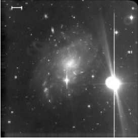
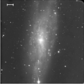
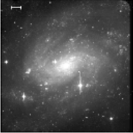
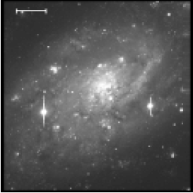
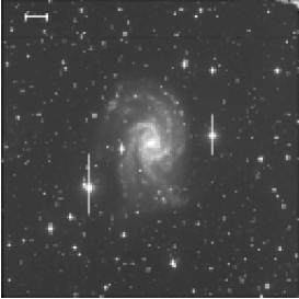
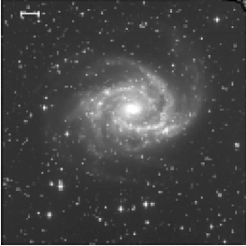
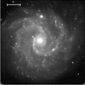
Observations of 21 nearby galaxies, listed in Table 1 of Paper1, were carried out with the Danish 1.54 m. telescope and DFOSC (Danish Faint Object Spectrograph and Camera) at the European Southern Observatory (ESO) at La Silla, Chile, and with the 2.56 m. Nordic Optical Telescope and ALFOSC (a DFOSC twin instrument), situated at La Palma, Canary Islands. The data consist of CCD images in the filters U,B,V,R,I and H. In the filters BVRI and H we typically made 3 exposures per galaxy of 5 minutes each, and 3 exposures of 20 minutes each in the U band. V-band images of the galaxies are shown in Figs. 4 and 5.
Both the ALFOSC and DFOSC were equipped with thinned, backside-illuminated 2 K2 Loral-Lesser CCDs. The pixel scale in the ALFOSC is 0.189″/pixel and the scale in the DFOSC is 0.40″/pixel, giving field sizes of and , respectively.
The seeing during the observations at La Silla was typically around 1.5 arcseconds as measured on V-band frames. On the images taken with the NOT the seeing was usually about 0.8 arcseconds. All observations used in this paper were conducted under photometric conditions.
During each observing run, photometric standard stars in the Landolt (landolt1992 (1992)) fields were observed for calibration of the photometry. Care was taken to include standard stars over as a wide a range in colours as possible, usually from to . Some of the Landolt fields were observed several times during the night at different airmass in order to measure the atmospheric extinction coefficients. For the flatfielding we used skyflats exposed to about half the dynamic range of the CCD, and in general each flatfield used in the reductions was constructed as an average of about 5 individual integrations, slightly offset with respect to each other in order to eliminate any stars.
3 Data reduction
The initial reductions of all CCD images (bias subtraction, flatfield correction, removal of bad columns) were done using the standard tools in IRAF222 IRAF is distributed by the National Optical Astronomical Observatories, which are operated by the Association of Universities for Research in Astronomy, Inc. under contract with the National Science Foundation. .
3.1 Standard calibrations
The instrumental magnitudes for the standard stars were obtained on the CCD images using the phot task in DAOPHOT (Stetson stet1987 (1987)) with an aperture radius of 20 pixels. The extinction correction was then applied directly to the raw instrumental magnitudes. The standard calibrations were carried out using the photcal package in IRAF with the transformation equations assumed to be of the linear form
Here the magnitudes written in capital letters correspond to the standard system, and magnitudes written with small letters are in the instrumental system, corrected for extinction only.
| NOT1 | NOT2 | DK1 | DK2 | |
| 14 | 32 | 45 | 35 | |
| 25 | 69 | 98 | 94 | |
| 0.039 | 0.029 | |||
| 1.109 | 1.111 | 1.100 | 1.104 | |
| 1.081 | 1.055 | 0.943 | 0.959 | |
| 1.012 | 1.027 | 1.013 | 1.014 | |
| 0.919 | 0.948 | 1.031 | 1.045 | |
| 0.082 | 0.005 | |||
| 0.154 | ||||
| 0.219 | 0.234 | 1.065 | 1.198 | |
| rms() | 0.008 | 0.034 | 0.019 | 0.037 |
| rms() | 0.013 | 0.042 | 0.019 | 0.032 |
| rms() | 0.042 | 0.043 | 0.050 | 0.041 |
| rms() | 0.017 | 0.033 | 0.030 | 0.024 |
The coefficients of the standard transformation equations are given in Table 1 for each of the four observing runs. NOT1 and NOT2 refer to observing runs at the Nordic Optical Telescope in May 1997 and October 1997, respectively, and DK1 and DK2 refer to runs at the Danish 1.54m telescope in September 1997 and February 1998. The CCD at the NOT was interchanged between the two runs which may explain the changes in the instrumental system from one run to the other, while the quantum efficiency of the CCD at the 1.54m telescope was notoriously unstable during the summer 1997/1998, and therefore the changes in the zero-point constants are hardly surprising. The rms scatter of the standard star observations relative to the standard system after the transformation is generally of the order of a few times 0.01 mag., with a slightly larger scatter in the U-B transformation. Thus, the accuracy of the standard transformations is sufficient for our purpose.
3.2 Reduction of science data
Following the initial reductions, the three exposures in each filter were aligned and combined into a single image, yielding an effective integration time of 15 minutes in BVRI and H and 60 minutes in U. As both the DFOSC and ALFOSC instruments can be rotated around the optical axis it was sometimes necessary to counter-rotate the individual exposures before they were combined (using the IRAF task rotate), even if attempts were made to position the instruments in the same way from night to night. This is due to the limited angular resolution of the encoders on the rotators. The necessary offsets and rotations were calculated by manually inspecting each frame and measuring the x-y coordinates of two selected stars using the IRAF task imexamine. By this method it was possible to align the images to a precision of about 0.1 pixel, accurate enough for our purpose. Flux conservation during the rotation was checked by comparing photometry on a synthetically generated image and on a rotated version of the same image. No deviations larger than 0.003 mag. were found.
The actual combination of the individual images was done using the task imcombine, with the reject option set to crreject in order to remove cosmic ray events. It was necessary to be particularly careful if the images to be combined had slightly different seeing, because the centres of bright stars could then be “rejected” by imcombine. We checked that this did not happen by also combining the images using no rejection at all and subtracting the two versions of the combined images from each other, making sure that no residuals were seen at the positions of stars. In general it was possible to avoid this problem by adjusting the snoise (“sensitivity noise”) parameter of imcombine.
As the first step towards detecting point-like objects we then created a smoothed version of a V-band image, using the median filtering task in IRAF and a 5 5 pixels box median filter. The median-filtered image was then subtracted from the original version, resulting in a residual image that contained no large-scale structure but only point sources superimposed on a uniform background. Point sources were finally located in the residual image using the daofind task in DAOPHOT.
Because star clusters are sometimes seen as slightly extended sources even at the distance of the galaxies in our sample, the photometry had to be obtained as aperture photometry rather than by PSF fitting (see also Östlin et al. ostlin1998 (1998)). The photometry was carried out directly on the combined images, and not on background subtracted images. In Paper1 it was argued that the accuracy obtained by this method was quite satisfactory. An aperture radius of 4 pixels was chosen for the determination of colour indices, while an aperture radius of 8 pixels was used to measure band magnitudes. It was shown in Paper1 (see also e.g. Holtzman et al. hol1996 (1996)) that aperture corrections tend to cancel out for colour indices, thus making it possible to measure accurate colours even with a quite small aperture.
The pixel size on the NOT images is half of that on the 1.54 m. images, but by coincidence the seeing on the NOT data was also, in general, twice as good as on the 1.54 m. data, so we used the same aperture radii in pixels for the NOT and 1.54 m. observations. Aperture corrections relative to the 20-pixels aperture radius used for the standard star observations were applied to the photometry, based on the assumption that the objects were point sources. The aperture corrections were derived from photometry of a few bright, isolated stars using the mkapfile task in DAOPHOT, and amounted in general to a few tenths of a magnitude. The photometry was corrected for Galactic foreground reddening using the extinction values given in the RC3 catalogue (de Vaucouleurs et al. vau91 (1991)).
3.3 Identification of star clusters

In short, young star cluster candidates were identified as compact bright, blue objects without any emission. The specific criteriae invoked to select cluster candidates were the following:
The first criterion was that the objects should have . In this way most foreground stars are eliminated, as demonstrated in Fig. 1 which shows colour-magnitude diagrams for objects in the field containing the galaxy NGC 2997. The NGC 2997 field is relatively rich in foreground stars, while the galaxy itself occupies only the central part of the frame, and therefore this field serves as an illustrative example. The difference between the colour-magnitude diagrams of the central part of the field (where the galaxy is located) and the outer parts (only foreground) is striking. In fact some of the foreground stars are slightly bluer than , so the limit is not completely rigorous and was adjusted slightly from case to case by inspecting diagrams like the one in Fig. 1. A colour of 0.45 for a star cluster corresponds to an age of about 500 Myr (Girardi et al. girardi1995 (1995)), so we are really just sampling young objects.
Secondly, the cluster candidates were divided into two groups, a “red” group with and a “blue” group with , and an absolute magnitude limit was applied. For a given mass, clusters in the “blue” group will be more luminous than clusters in the “red” group, and therefore a brighter magnitude cut-off could be applied to the “blue” clusters. Specifically, the limits were set to for the “red” group and to for the “blue” group (distance modulii for the galaxies are given in Paper1).
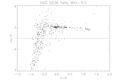
Third, it was necessary to exclude HII regions. In Fig. 2 we show vs. for all objects brighter than in the NGC 5236 field, chosen as an example because of the large number of sources in this galaxy. The photometry was not standard calibrated, so the magnitude scale on the y-axis in Fig. 2 is purely instrumental. It is clear from Fig. 2 that the objects with an excess in appear around , while is rather constant for redder objects. Denoting the average value at by , we chose to cut away objects with . The limit could have been placed closer to , but by choosing a cut-off at 0.5 magnitudes below we allow for some scatter in the photometry as well.
Finally we did a visual inspection of the cluster candidates. In this way objects which were too extended or “fuzzy” to be star clusters were eliminated (typically star clouds or associations in the spiral arms of the galaxies).
n1313-Psf

n5236-Psf

n628-Psf

n1313-201

n5236-76

n628-274

n1313-379

n5236-175

n628-1171

n1313-574

n5236-199

n628-1880

n1313-627

n5236-347

n628-2283

Photometric data are given for each cluster in Table 4, along with the effective radius (in pc) as derived by ishape (Sec. 4). A few examples of clusters are shown in Fig. 3.
A table showing the total number of star clusters identified in each of the galaxies in our sample was given in Paper1, and we refer to that paper for a detailed discussion of the properties of the cluster systems.
NGC 45
NGC 247
NGC 300
NGC 628
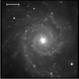
NGC 1156
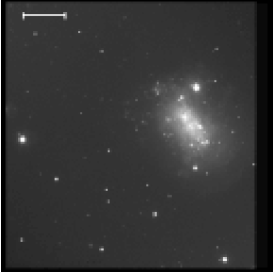
NGC 1313
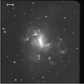
NGC 1493
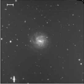
NGC 2403
NGC 2835
NGC 2997
NGC 3184
NGC 3621
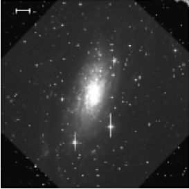
NGC 4395
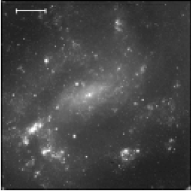
NGC 5204
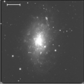
NGC 5236
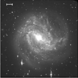
NGC 5585
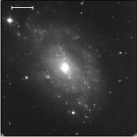
NGC 6744
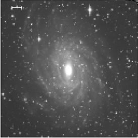
NGC 6946
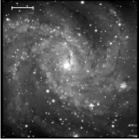
NGC 7424
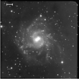
NGC 7741
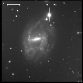
NGC 7793
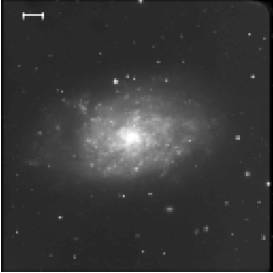
4 Tools for synthetic image generation and analysis
It is a complicated problem to carry out photometry on star clusters located within spiral galaxies, partly because of the strongly varying background, and partly because the clusters are not perfect point sources. The measurements are subject to many potential errors, and it is essential to check the photometry carefully and get a realistic idea of the achievable accuracy. One way to do this is to carry out experiments with artificial objects, which can be added at any desired position in the image and remeasured using the photometric method of choice. In order to give realistic estimates of the photometric errors the artificial objects should, of course, resemble the real objects as closely as possible.
We have developed a number of tools to be used in the analysis of this type of image data. The two most important ones, which will be described below are
-
•
mksynth - generates a synthetic image by adding artificial sources to a uniformly illuminated sky background.
-
•
ishape - which finds the intrinsic shape of extended sources by modeling them as one of several available analytic models. The parameters of the analytic model are adjusted until the best fit between the observed profile and the model convolved with the PSF of the image is obtained.
In practice these two algorithms (together with some more general image processing functions) are built into one stand-alone programme333 The programme containing the routines, (for historical reasons called baolab), is available at the following WWW address: http://www.astro.ku.dk/∼soeren/baolab/ , so that they can share common routines to handle user-definable parameters, read and write FITS images etc.
We have not included a task to generate the PSF itself from an image. This must be done using some other programme, such as the psf and seepsf tasks in DAOPHOT. We refer to the IRAF and DAOPHOT documentation for more details on these topics.
4.1 mksynth
This algorithm generates synthetic images which are as similar to real data as possible, including a “sky background” with gaussian photon shot noise. Stars are generated not just by adding a scaled PSF but rather by a process similar to that by which the photons arrive in a real CCD image during an integration. Thus, in contrast to other popular algorithms for adding synthetic stars to an image (such as addstar in DAOPHOT), mksynth generates a complete synthetic image from scratch, including a noisy background if desired. The PSF can be modeled as one of several analytic profiles (see Sect. 4.2), or read from a FITS file.
One of the major forces of the algorithm is that it allows a great flexibility in the generation of synthetic images, through a number of user-definable parameters. The coordinates and magnitudes of the synthetic objects can be read from a file, or generated at random.
Tests have shown that synthetic images generated by mksynth have very realistic noise characteristics, and it is possible to generate synthetic images which resemble real CCD images very closely. mksynth was described and tested more fully (although in a more primitive version) by Larsen (larsen1996 (1996)).
4.2 ishape
| FITRAD = float | Fitting radius (in pixels) |
|---|---|
| CENTERRAD = float | Centering radius |
| CLEANRAD = float | Cleaning radius |
| CTRESH = float | Cleaning threshold (in ) |
| SHAPE = string | Which model to use |
| ELLIPTICAL = YES/NO | Fit elliptical model? |
| EPADU = float | Conversion factor of CCD image |
| RON = float | Read-out noise |
| RESIMAGE = string | File with residual image |
| REPLACE = YES/NO | Remove the object from the original image? |
| KEEPLOG = YES/NO | Keep a log file? |
| LOGFILE = string | Name of log file (if KEEPLOG=YES) |
ishape can be used to estimate the intrinsic shape parameters of extended objects in a digital image with a known PSF. The algorithm is designed to work in the domain of “slightly” extended objects which can be modeled as simple analytic functions, i.e. objects with a size roughly equal to or smaller than the PSF. Conventional deconvolution algorithms are not designed for this type of problem. None of the “first-generation” deconvolution algorithms such as the Maximum Entropy Principle (Burch et al. burch1983 (1983)) and the Richardson-Lucy algorithm (Richardson richard1972 (1972), Lucy lucy1974 (1974)) handled point-like sources well at all. More recent “two-channel algorithms” (Lucy lucy1994 (1994), Magain et al. magain1998 (1998)) model the image as consisting of a smoothly varying background and a number of -functions. The two-channel algorithms seem to work quite well in many cases, being able to separate point sources and obtain deconvolved images of photometric quality, but they are not able to treat objects which are only nearly point-like. Therefore we feel it is worthwhile to spend some space describing our algorithm which handles this specialised, but for our work important case. We have used ishape to derive intrinsic radii for star clusters in other galaxies, but one could also imagine other areas of work where the algorithm might be useful, for example in the study of distant galaxies which are just barely resolved.
The analytic profiles by which ishape models the sources are:
| GAUSS: | (1) | ||||
| MOFFAT15: | (2) | ||||
| MOFFAT25: | (3) | ||||
| KINGc: | (6) | ||||
| LUGGER: | (7) | ||||
| HUBBLE: | (8) | ||||
| DELTA: | (9) |
Here is given by the equation , where the constants , and depend on the major axis, ellipticity and orientation of the model, and and are the coordinates relative to the centre of the profile.
For the KING models, the concentration parameter444For convenience, we define the concentration parameter as where is the tidal radius and is the core radius. In the literature it is customary to define . may assume the values 5, 15, 30 and 100. Note that the HUBBLE model is equal to a KING model with infinite concentration parameter. The MOFFAT models are similar to the profiles used by Elson et al. (elson1987 (1987)) to fit young LMC clusters, with their profile corresponding to the MOFFAT15 model and to the MOFFAT25 model. Elson et al. (1987) found for their sample of LMC clusters. Unlike the KING models, the MOFFAT functions never reach a value of 0, but both the MOFFAT15 and MOFFAT25 functions share the desirable property that their volume is finite so that a well-defined effective radius exists. Clearly, the DELTA model is normally of little use, and is mostly used internally by ishape. The code can easily be extended to include other models as long as they can be described as simple analytic functions of the parameter .
Denoting the observed image of an object , the PSF with , the intrinsic shape with and the convolution of the two , the algorithm finds by minimising the function:
| (10) |
is the position of the object, and represent the amplitude (brightness) and the background level, and , and are the FWHM along the major and minor axes and the position angle. is the statistical uncertainty on the pixel value at the position , and is a weighting function. The summation (10) is carried out over all the elements of the image area considered (typically a rather small section around the object).
The actual implementation of the minimisation of Eq. (10) is somewhat more complicated than just minimising as a function of all seven parameters at once, and particular care is taken to evaluate the convolution as few times as possible. Only the parameters and affect the the actual shape of the convolved profile, so one might think of as a function of these three parameters only, with the minimisation of the remaining parameters ( position, the amplitude and background ) being carried out implicitly for each choice of and . The function is minimised using the “downhill simplex” algorithm (Press et al. press (1992)) which has the advantage of being simple and robust. The initial guesses are partly user-definable, but tests have shown that as long as convergence is reached, the results are insensitive to the initial guesses.
The result of the fit is given as a FWHM along the major axis and an axis ratio and orientation, but the FWHM may easily be converted to an effective radius (containing half the total cluster light) for all profiles except the HUBBLE and LUGGER profiles.
Both in mksynth and ishape, the arrays containing image data are in reality stored internally with a resolution 10 times higher than the actual image resolution. However, when calculating the (Eq. (10)) the arrays are rebinned to the original resolution.
The weighting array is introduced in order to reduce the effect of bad pixels, cosmic ray events, nearby stars etc. The weights are derived from the input image before the iterations are started by calculating the standard deviation among the pixels located in concentric rings around the centre of the object, and assigning a weight to each pixel which is inversely proportional to its deviation from the mean of the pixels located in the same ring. If the deviation of is smaller than one then the corresponding weight is set equal to 1, and if the deviation is larger than a user specified parameter (CTRESH) then is set equal to 0, effectively rejecting that pixel. For small distances from the centre of the profile the statistics will become poor and hence all weights are set equal to 1 for distances smaller than a user-specified limit (CLEANRAD). It is clear that this method of assigning weights works best for images where the sources are more or less circularly symmetric - if this is not the case, then the CLEANRAD parameter should be set to a large value so that all pixels are assigned equal weights.

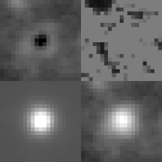
Examples of the output produced by ishape are shown in Fig. 6. In the left part of the figure the cluster was modeled as a MOFFAT15 function, and in the right part of the figure the cluster was modeled as a DELTA function. In each set of four images the original cluster is shown in the lower right corner, the final model convolved by the PSF () is seen to the lower left, the fit residuals are given to the upper left, and the weighting array is shown to the upper right. Note how structures in the background correspond to regions that are assigned a low weight, indicated by dark areas in the weighting array. In a typical situation it would have been adequate to choose a smaller fitting radius (and thereby reduce the computation time), but in this example we have extended the fitting radius to 11 pixels in order to demonstrate how the star near the upper left corner affects the weighting array.
From Fig. 6 we note two things: First, the fit is improved enormously by allowing the model to be extended as opposed to the DELTA model, which corresponds to subtraction of a pure PSF. Hence, the object is clearly recognised as an extended source. Second, considering that the fitting radius in this example is as large as 11 pixels, the residuals resulting from modeling the cluster as an extended source show no other systematic variations than what can be attributed to background variations. In this particular example the FWHM along the major axis of the MOFFAT15 function was found to be 1.67 pixels, and the FWHM of the PSF was 4.1 pixels.
4.3 Tests of ishape
Before applying ishape to data, it is of interest to know how reliably the elongation and major axis of small objects in a CCD image can be reconstructed.


| Mag. | 18.7 | 19.4 | 20.4 |
|---|---|---|---|
| Inner field | 142 | 79 | 36 |
| Outer field | 157 | 88 | 40 |
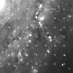
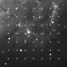
This was tested by generating a synthetic image with a number of objects with known shape parameters and then remeasuring them using ishape. First, 49 test objects were generated by convolving the PSF measured on a V-band CCD image of the galaxy NGC 5236 with a number of MOFFAT15 models with major axis FWHMs in the range 0 - 3 pixels and axis ratios between 0 and 1. A synthetic image with all of the 49 test objects was then generated using mksynth, and the synthetic image was finally added to a section of the original image of NGC 5236. This procedure was repeated for synthetic objects of magnitudes 18.7, 19.4 and 20.4 at two positions within NGC 5236 (see Fig. 7). Finally, ishape was run on the test images, and the shape parameters derived by ishape were compared with the input values.
The results are shown in Figs. 8 (inner field) and 9 (outer field). The plots in the left column show the measured FWHM versus the input values, and those in the right column show the measured axis ratio versus the input values. The correlations are more tight for the outer field, implying that the high noise level and stronger background fluctuations in the bright disk near the centre of NGC 5236 limit ishape’s ability to reconstruct the shape of the objects. The median S/N ratios for the test objects calculated by ishape are given in Table 3, and as expected the objects in the inner field have somewhat poorer S/N ratios. It is interesting to note that when sufficient signal is present the FWHM is recovered with quite high precision even down to very small values, below FWHM = 0.5 pixels. The FWHM of the PSF itself was 4 pixels, which means that objects with sizes as small as about 10% of that of the PSF can be recognised as extended objects with good confidence.
From Table 3 and Figs. 8 and 9 we estimate that the S/N ratio should be greater than about 50 in order to obtain reasonably accurate shape parameters, although there are probably also many other factors which affect the results, such as the presence of nearby neighbours, crowding in general and the smoothness of the background. The axis ratio is generally somewhat more uncertain than the FWHM, although the scatter would decrease if the more compact objects were excluded from the plot. We will not discuss axis ratios further in this paper, but remark that the elongation might be used as a criterion to look for double clusters.

In the previous tests we had the advantage of knowing the intrinsic shape of the synthetic clusters in advance. This will usually not be the case in practice, so we should also examine how sensitive the derived cluster sizes are to a particular choice of model. In this study we have used the MOFFAT15 profile to model the clusters because of its similarity to the models that were found to fit young LMC clusters by Elson et al. (elson1987 (1987)), but other choices might be as good. In particular, the classical models by King (king1962 (1962)) are known to fit galactic globular clusters very well. We therefore generated another set of synthetic images in the same way as for the previously described ishape tests, but now with Gaussian, King() and King() input models. The cluster sizes were then remeasured using ishape and the MOFFAT15 model. The experiment was carried out only for the outer NGC 5236 field, and for one set of images (corresponding to the brightest set used in the previous tests).
The results of this test are shown in Fig. 10 for FWHM (left) and half-light radii (right). Though some systematic model dependencies are evident for the FWHM values, half-light radii are reproduced quite well by the MOFFAT15 model, regardless of the input model. A related result was obtained by Kundu & Whitmore (kw1998 (1998)) who found that effective radii derived by fits to a King model were quite insensitive to the adopted concentration parameter. We may thus conclude that the derived effective radii are not very sensitive to the choice of model, and even if the true cluster profiles are closer to King profiles the choice of the MOFFAT15 model will not introduce any large systematic errors.
5 Completeness corrections

After the discussion of software tools we now return to YMCs. In Paper1 the total numbers of clusters detected in each of the 21 galaxies in our sample were listed, and we also attempted to correct the raw numbers for completeness effects. Here the completeness corrections will described in a bit more detail than in Paper1.
The fraction of clusters that are not detected may be estimated by adding artificial clusters to the images using a programme like mksynth and then checking how many of them are recovered by DAOFIND. This kind of completeness test is well documented in the literature for globular clusters in elliptical galaxies (Forbes forbes1996 (1996), Kissler-Patig et al. kiss1996 (1996)) and also in other contexts. The artificial objects are usually added at random positions, which is a reasonable thing to do because this is also how the actual sources under study are distributed.
However, in our case the problem is somewhat different because YMCs are not distributed at random within their host galaxies. Instead, the clusters (in particular those in the “blue” group, i.e. the youngest ones) tend to be located in or near the spiral arms where they are much more likely to drown in background fluctuations, and hence a completeness test based on objects distributed at random is likely to underestimate the completeness correction.
Our approach has been to add the artificial objects “close” to the detected objects, adding 5 clusters at random positions within a radial range of 20 - 70 pixels from each detected cluster. The objects were added to the , and band frames using the mksynth task, and it was then required that they were refound by daofind and that phot was able to obtain magnitudes in all three filters. The completeness tests were carried out for magnitudes down to the limit at intervals of 0.5 magnitudes, and a completeness correction was then calculated for each magnitude interval. The procedure was repeated twice, for point sources and for extended objects modeled as a MOFFAT15 profile with an effective radius corresponding to pc convolved with the PSF. Finally, the number of clusters actually detected in each magnitude interval was corrected by the completeness correction calculated for that interval, and the corrected numbers are given in Paper1 for the point-source as well for the extended-source corrections.
Completeness tests were carried out only for the galaxies with more than 20 clusters. Many of the cluster-poor galaxies contained only a handful or fewer clusters, and it makes little sense to attempt to apply completeness corrections to such small numbers.
The estimated completenesses for sources in the 6 galaxies with more than 20 clusters are shown graphically in Fig. 11 as a function of absolute visual magnitude. Note the striking difference between point sources (upper panel) and extended sources (lower panel), in particular in NGC 2997. The number of detections in NGC 2997 in the extended source experiment actually drops to 0 at , which indicates that in NGC 2997 we simply cannot make a realistic estimate of how many objects the galaxy contains down to a limit of . The other galaxies in our sample were either more nearby, or they were observed at the NOT rather than the 1.54m telescope (and therefore with better image quality), so with the exception of two more galaxies (NGC 7424 and NGC 1493, see Paper1) the incompleteness corrections should be smaller than those for NGC 2997.
6 Resolving YMCs in the galaxies
The ishape algorithm was applied to all the star clusters identified as described in Sect. 3.3. For the shape model the MOFFAT15 profile was chosen because of its similarity with the models adopted by Elson et al. (elson1987 (1987)), and the PSF was generated using DAOPHOT. The cleaning radius was set to 2 pixels and the fitting radius to 4 pixels, and the CTRESH parameter was set to 2.


The effective radii were derived both on and band images for the 6 most cluster-rich galaxies in order to check the results. In Fig. 12 the effective radii (in pixel units) derived by ishape from and band frames are plotted against each other for objects with S/N 50, leaving out about 20% of the objects. If objects with lower S/N were included, the scatter was found to increase somewhat, although the correlations in Fig. 12 would remain evident.
As another test, radii were derived for sources in the NGC 5236 frame with and . Most of these objects are expected to be foreground stars, and they are indeed distributed quite uniformly across the CCD frame. Fig. 13 shows the distribution for all such objects located within the central pixels of the image, roughly corresponding to the area covered by the galaxy. For convenience, the effective radii have been converted to parsec. It can be seen from Fig. 13 that ishape finds pc (0.05″) for the vast majority of the objects with , in agreement with the assumption that they are in fact foreground stars. The fact that foreground stars appear virtually unresolved by ishape adds confidence to the algorithm’s ability to recognise extended objects.
The number of clusters in most of the galaxies are really too sparse that it makes sense to discuss the distributions for individual galaxies. However, Fig. 14 shows histograms for two of the most cluster-rich galaxies, NGC 5236 and NGC 1313. These are also the two most nearby galaxies, at and respectively (see Paper1). Separate histograms are given for the “red” (U-B ) and “blue” (U-B ) cluster samples. Several systematic effects might influence the observed distributions, for example the fact that the most extended clusters are detected with a much lower efficiency, and one should be careful not to overinterpret the data in Fig. 14. Nevertheless, the objects in the “blue” sample generally seem to be less concentrated, which might imply that many of the blue objects are loosely bound associations that do not survive long, rather than bound clusters. It is emphasised, however, that this statement could only be justified by a more detailed study of the structure of the objects, something that is not feasible from ground-based observations. Fig. 14 also seems to indicate that many of the objects in NGC 5236 are more concentrated than those in NGC 1313, although the statistics are poor for the latter galaxy.
From the discussion in Sect. 4.3 and Fig. 12 the uncertainty on the cluster radii is estimated to be about 0.5 pixels. 1 DFOSC pixel () corresponds to about 7 pc at the distance of NGC 5236 and NGC 1313, so we expect an uncertainty of about 4 pc on the individual cluster radii in Fig. 14, as indicated by the horizontal error bars. The fact that we do not observe any lower limit in the distribution may be an effect of the limited resolution, causing clusters with larger radii to scatter into the low region, but the lower limit in our sample cannot be higher than a few pc.
How do the sizes of the clusters discussed here compare with other results? Accurate measurements of cluster sizes are available only in the Milky Way and in the LMC. Most globular clusters in the Milky Way have pc with a peak in the distribution at about 3 pc, although clusters with up to pc exist (Harris harris1996 (1996)). Elson et al. (elson1987 (1987)) found typical half-mass radii for young LMC clusters in the range 5 - 15 pc, corresponding to values between 4 and 12 pc (Spitzer spitz1987 (1987)).
Effective radii have been estimated also for young clusters in the Antennae by Whitmore & Schweizer (ws1995 (1995), WS95) using HST/WFPC data, and in the merger remnant NGC 7252 (Whitmore et al. whit93 (1993)), in both cases by assuming gaussian cluster profiles. WS95 found an average of 12 pc for the Antennae clusters, but new WFPC/2 data lead to a revised mean value of pc (Whitmore et al. whit99 (1999)). In the case of NGC 7252, Whitmore et al. (whit93 (1993)) found a mean effective radius of 9.9 pc for clusters located at distances larger than 3.5″ from the centre of NGC 7252. Östlin et al. (ostlin1998 (1998)) used the model profile of Lugger et al. (lug1995 (1995)) to estimate core radii (one half times the FWHM) for YMCs in the blue compact galaxy ESO 338-IG04, and found a distribution that peaked at 2.5 pc with all clusters having core radii less than 10 pc. The Lugger et al. (lug1995 (1995)) profile does not have a well-defined effective radius, but Östlin et al. (ostlin1998 (1998)) also found that if the clusters were instead fitted with gaussian profiles (for which the core radius equals ) the core radii were about 2 times larger than for the Lugger et al. (lug1995 (1995)) profiles, so their distribution should peak at about 5 pc and have an upper limit at 20 pc.
Our observed distributions thus seem to resemble those observed for YMCs in other galaxies quite well. We note, however, that the effective radii have been estimated by a variety of methods in the different studies, and this could account for some of the differences. The effective radii for the YMCs in our sample are also comparable with those of Galactic globular clusters and young LMC clusters.
The velocity dispersion in a star cluster or OB association is typically of the order of 1 - 10 km/sec, so an unbound object will expand by 1 - 10 pc / Myr. A U-B colour of corresponds to an age of about 50 Myr (Girardi et al. girardi1995 (1995)), so most of the objects in the “red” group would have expanded to sizes much larger than what is observed and would have effectively disappeared if they were not gravitationally bound. Like all star clusters they will eventually be subject to dynamical erosion, but this acts on much longer timescales and the lifetimes are difficult to estimate without a detailed knowledge of the morphology of individual clusters and their orbits within the host galaxies.
7 Summary and conclusions
The data reductions applied to the sample of 21 galaxies presented in Paper1 have been extensively discussed, in particular the algorithm ishape which is a useful tool for the analysis of compact objects. Tests show that ishape is able to recognise extended objects with good confidence, down to a FWHM of about 1/10 of the FWHM of the PSF itself.
Completeness tests of the cluster samples of the 6 most cluster-rich galaxies were carried out using mksynth, and it was demonstrated that the completeness depends strongly on the extent of the objects.
Using ishape, effective radii of YMCs were obtained, and the distributions in NGC 1313 and NGC 5236 were studied in more detail. We found effective radii of the YMCs in these two galaxies in the range 0 - 20 pc, in good agreement with results obtained for YMCs in other galaxies, and also similar to those of old globular clusters in the Milky Way and YMCs in the LMC. Some of the objects with U-B may be loosely bound associations, while objects with U-B (older than Myr) are orders of magnitude older than their crossing times, and we may thus conclude that they are genuine clusters. Many of them are significantly more massive than any open cluster in the Milky Way, and may well evolve into objects resembling the old globular clusters seen in the halo of the Milky Way and other galaxies today.
Acknowledgements.
This research was supported by the Danish Natural Science Research Council through its Centre for Ground-Based Observational Astronomy. The valuable comments of the referee, Dr. Jon Holtzman, which helped improve this paper are appreciated. This research has made use of the NASA/IPAC Extragalactic Database (NED) which is operated by the Jet Propulsion Laboratory, California Institute of Technology, under contract with the National Aeronautics and Space Administration.References
- (1) Burch S.F., Gull S.F., Skilling J. 1983, Computer Vision, Graphics and Image Processing 23, 113
- (2) Elson R.A.W., Fall M.S., Freeman K.C. 1987, ApJ 323, 54
- (3) Fischer P., Welch D.L., Cote P., Mateo M., Madore B.F. 1992, AJ 103, 857
- (4) Forbes D. A. 1996, AJ 112, 954
- (5) Girardi L., Chiosi C., Bertelli G., Bressan A. 1995, A&A 298, 87
- (6) Harris W.E. 1996, AJ 112, 1487
- (7) Holtzman J.A., Watson A.M., Mould J.R. et al. 1996, AJ 112, 416
- (8) King I. 1962, AJ 67, 471
- (9) Kissler-Patig M., Richtler T., Hilker M. 1996, A&A 308, 704
- (10) Kundu A., Whitmore B.C. 1998, AJ 116, 2841
- (11) Landolt A.U. 1992, AJ 104, 340
- (12) Larsen S.S. 1996, Masters Thesis, Copenhagen University Observatory
- (13) Larsen S.S. & Richtler T. 1999 A&A 345, 59 (Paper1)
- (14) Lucy L.B. 1974, AJ 79, 745
- (15) Lucy L.B. 1994, in: The Restoration of HST images and Spectra II, eds. Hanish, R.J. & While, R.L.
- (16) Lugger P., Cohn H., Grindlay J. 1995, ApJ 439, 191
- (17) Magain P., Courbin F., Sohy S. 1998, ApJ 494, 472
- (18) Press W.H., Teukolsky S.A., Vetterling W.T., Flannery B.P., Numerical Recipes in C/Fortran, second ed. Cambridge University Press 1992
- (19) Richardson W.H. 1972, J. Opt. Soc. Am. 62, 55
- (20) Spitzer L. 1987, Dynamical Evolution of Globular Clusters, Princeton University Press
- (21) Stetson P. 1987, PASP 99, 191
- (22) de Vaucouleurs G., de Vaucouleurs A., Corwin H.G. et al. 1991, Third Reference Catalogue of Bright Galaxies, Springer-Verlag New York (RC3)
- (23) Whitmore B.C., Schweizer F., Leitherer C. et al. 1993, AJ 106, 1354
- (24) Whitmore B.C., Schweizer F., 1995, AJ 109, 960 (WS95)
- (25) Whitmore B.C., Zhang Q., Leitherer C., Fall M., Schweizer F. 1999, BAAS 31, 12.05
- (26) Östlin G., Bergvall N., Rönnback J. 1998, A&A 335, 85
| ID | (2000.0) | (2000.0) | U-B | B-V | V-I | |||
|---|---|---|---|---|---|---|---|---|
| n45-121 | 645,685 | 0:14:15.10 | -23:13:24.9 | -9.94 | -0.64 | 0.34 | 0.68 | 32.8 |
| n45-271 | 1104,1034 | 0:14:01.74 | -23:11:12.8 | -8.77 | -0.14 | 0.43 | 0.66 | 4.7 |
| n45-341 | 1030,1203 | 0:14:03.72 | -23:10:05.8 | -8.51 | -0.31 | 0.09 | 0.33 | 27.6 |
| n247-508 | 949,1057 | 0:47:09.29 | -20:45:30.2 | -8.63 | -0.28 | 0.33 | 0.58 | 37.7 |
| n247-871 | 1327,1715 | 0:46:58.25 | -20:41:16.0 | -10.24 | -0.67 | 0.02 | 0.39 | 4.9 |
| n247-899 | 985,1784 | 0:47:07.76 | -20:40:45.5 | -9.38 | -0.06 | 0.16 | 0.46 | 6.5 |
| n300-221 | 1319,342 | 0:54:43.48 | -37:45:33.1 | -8.62 | -0.16 | 0.28 | 0.79 | 9.8 |
| n300-566 | 1822,579 | 0:54:26.71 | -37:44:03.6 | -8.69 | -0.35 | 0.18 | 0.42 | 4.7 |
| n300-1273 | 393,919 | 0:55:13.74 | -37:41:39.9 | -9.85 | -0.64 | 0.20 | 0.37 | 4.6 |
| n628-92 | 1297,93 | 1:36:38.74 | 15:44:17.2 | -10.52 | -0.78 | -0.02 | 0.27 | 12.8 |
| n628-168 | 1151,170 | 1:36:40.63 | 15:44:31.3 | -10.03 | -0.90 | -0.11 | 0.19 | 30.4 |
| n628-201 | 1306,209 | 1:36:38.64 | 15:44:38.8 | -8.92 | -0.31 | 0.22 | 0.51 | 23.2 |
| n628-274 | 844,306 | 1:36:44.61 | 15:44:56.2 | -11.33 | -0.83 | 0.04 | 0.43 | 10.3 |
| n628-544 | 649,579 | 1:36:47.15 | 15:45:46.7 | -11.31 | -0.79 | 0.03 | 0.36 | 43.9 |
| n628-549 | 1033,584 | 1:36:42.20 | 15:45:48.3 | -10.01 | -0.58 | 0.32 | 0.64 | 29.0 |
| n628-563 | 1250,592 | 1:36:39.40 | 15:45:50.1 | -9.84 | -0.62 | 0.02 | 0.50 | 1.0 |
| n628-622 | 1141,636 | 1:36:40.81 | 15:45:58.2 | -9.65 | -0.64 | 0.00 | 0.26 | 5.2 |
| n628-681 | 1414,667 | 1:36:37.30 | 15:46:04.4 | -8.59 | -0.19 | 0.12 | 0.30 | 16.9 |
| n628-824 | 1461,747 | 1:36:36.70 | 15:46:19.4 | -8.61 | -0.22 | 0.08 | 0.13 | 5.0 |
| n628-947 | 1208,822 | 1:36:39.97 | 15:46:32.9 | -9.80 | -0.83 | 0.03 | 0.56 | 43.4 |
| n628-963 | 447,829 | 1:36:49.79 | 15:46:33.0 | -8.59 | -0.36 | 0.09 | 0.33 | 3.2 |
| n628-976 | 1485,836 | 1:36:36.40 | 15:46:36.0 | -9.84 | -0.42 | 0.12 | 0.61 | 43.5 |
| n628-1007 | 1003,858 | 1:36:42.62 | 15:46:39.3 | -9.94 | -0.77 | 0.05 | 0.50 | 23.2 |
| n628-1099 | 1549,898 | 1:36:35.58 | 15:46:47.7 | -9.61 | -0.58 | 0.15 | 0.81 | 17.8 |
| n628-1101 | 489,899 | 1:36:49.25 | 15:46:46.1 | -8.81 | -0.03 | 0.15 | 0.51 | 3.8 |
| n628-1140 | 492,921 | 1:36:49.22 | 15:46:50.2 | -9.87 | -0.42 | 0.13 | 0.69 | 1.8 |
| n628-1171 | 807,941 | 1:36:45.16 | 15:46:54.5 | -9.58 | -0.49 | 0.24 | 0.69 | 17.0 |
| n628-1285 | 1340,996 | 1:36:38.29 | 15:47:05.6 | -9.92 | -0.81 | 0.08 | 0.20 | 31.5 |
| n628-1340 | 619,1025 | 1:36:47.59 | 15:47:09.8 | -11.04 | -0.75 | 0.01 | 0.50 | 29.1 |
| n628-1348 | 603,1028 | 1:36:47.80 | 15:47:10.4 | -9.61 | -0.63 | 0.10 | 0.24 | 1.8 |
| n628-1451 | 1304,1067 | 1:36:38.76 | 15:47:18.8 | -10.24 | -0.79 | -0.01 | 0.22 | 31.5 |
| n628-1455 | 1485,1069 | 1:36:36.43 | 15:47:19.4 | -9.85 | -0.48 | 0.20 | 0.77 | 8.7 |
| n628-1559 | 1400,1115 | 1:36:37.53 | 15:47:27.9 | -9.60 | -0.53 | 0.09 | 0.52 | 23.8 |
| n628-1587 | 1338,1130 | 1:36:38.33 | 15:47:30.6 | -8.80 | -0.16 | 0.26 | 0.58 | 17.4 |
| n628-1591 | 1516,1131 | 1:36:36.03 | 15:47:31.0 | -9.51 | -0.67 | 0.07 | 0.67 | 29.0 |
| n628-1690 | 1266,1195 | 1:36:39.26 | 15:47:42.6 | -10.22 | -0.83 | -0.02 | 0.26 | 29.7 |
| n628-1780 | 684,1251 | 1:36:46.78 | 15:47:52.1 | -9.83 | -0.62 | 0.07 | 0.33 | 21.1 |
| n628-1807 | 1282,1268 | 1:36:39.07 | 15:47:56.2 | -8.91 | -0.29 | 0.13 | 0.32 | 13.5 |
| n628-1828 | 1773,1283 | 1:36:32.73 | 15:47:59.8 | -9.60 | -0.46 | 0.13 | 0.47 | 14.3 |
| n628-1880 | 965,1316 | 1:36:43.16 | 15:48:04.7 | -9.12 | -0.23 | 0.19 | 0.65 | 0.8 |
| n628-1885 | 1178,1318 | 1:36:40.41 | 15:48:05.4 | -9.78 | -0.33 | 0.24 | 0.75 | 4.3 |
| n628-1926 | 1040,1348 | 1:36:42.20 | 15:48:10.7 | -9.65 | -0.61 | 0.02 | 0.59 | 3.0 |
| n628-1963 | 1049,1377 | 1:36:42.08 | 15:48:16.2 | -10.55 | -0.76 | 0.04 | 0.58 | 24.8 |
| n628-2120 | 1142,1501 | 1:36:40.90 | 15:48:39.4 | -9.90 | -0.49 | 0.11 | 0.75 | 12.8 |
| n628-2244 | 674,1614 | 1:36:46.95 | 15:48:59.7 | -11.33 | -0.68 | 0.11 | 0.46 | 3.5 |
| n628-2283 | 1482,1642 | 1:36:36.53 | 15:49:06.3 | -8.54 | -0.22 | 0.21 | 0.46 | 10.5 |
| n628-2408 | 1048,1830 | 1:36:42.15 | 15:49:40.6 | -9.44 | -0.02 | 0.20 | 0.55 | 2.1 |
| n1156-296 | 1414,883 | 2:59:41.83 | 25:13:39.0 | -9.38 | -0.14 | 0.20 | 0.31 | 0.2 |
| n1156-310 | 1333,903 | 2:59:42.95 | 25:13:42.6 | -8.74 | -0.05 | 0.26 | 0.69 | 5.8 |
| n1156-331 | 1488,927 | 2:59:40.82 | 25:13:47.4 | -9.68 | -0.62 | 0.05 | 0.32 | 23.2 |
| n1156-348 | 1480,944 | 2:59:40.93 | 25:13:50.6 | -11.10 | -0.75 | 0.21 | 0.73 | 33.6 |
| n1156-356 | 1776,950 | 2:59:36.86 | 25:13:52.4 | -9.02 | -0.01 | 0.39 | 0.67 | 6.4 |
| n1156-361 | 1482,954 | 2:59:40.91 | 25:13:52.5 | -10.88 | -0.83 | 0.05 | 0.57 | 9.7 |
| n1156-403 | 1456,1005 | 2:59:41.27 | 25:14:01.9 | -8.98 | -0.26 | 0.32 | 0.62 | 8.5 |
| n1156-433 | 1345,1032 | 2:59:42.81 | 25:14:06.7 | -9.12 | -0.20 | 0.37 | 0.80 | 20.8 |
| n1156-441 | 1324,1041 | 2:59:43.10 | 25:14:08.3 | -9.47 | 0.32 | 0.31 | 0.54 | 14.6 |
| ID | (2000.0) | (2000.0) | U-B | B-V | V-I | |||
|---|---|---|---|---|---|---|---|---|
| n1156-442 | 1372,1042 | 2:59:42.44 | 25:14:08.6 | -9.52 | -0.49 | -0.01 | 0.29 | 15.2 |
| n1156-476 | 1329,1067 | 2:59:43.03 | 25:14:13.2 | -9.53 | -0.41 | 0.09 | 0.40 | 3.7 |
| n1156-496 | 1426,1085 | 2:59:41.70 | 25:14:16.8 | -9.68 | -0.65 | 0.10 | 0.47 | 6.4 |
| n1156-513 | 1404,1099 | 2:59:42.01 | 25:14:19.3 | -10.01 | -0.53 | 0.12 | 0.40 | 7.1 |
| n1156-549 | 1455,1125 | 2:59:41.31 | 25:14:24.3 | -9.74 | -0.12 | 0.25 | 0.48 | 20.7 |
| n1156-554 | 1269,1129 | 2:59:43.87 | 25:14:24.6 | -9.74 | -0.42 | 0.33 | 0.64 | 24.0 |
| n1156-555 | 1262,1130 | 2:59:43.97 | 25:14:24.8 | -9.69 | -0.72 | 0.04 | 0.39 | 18.9 |
| n1156-561 | 1351,1133 | 2:59:42.74 | 25:14:25.5 | -11.07 | -0.45 | 0.16 | 0.57 | 14.8 |
| n1156-610 | 1347,1172 | 2:59:42.80 | 25:14:32.8 | -10.12 | -0.51 | 0.22 | 0.85 | 16.3 |
| n1156-619 | 1370,1181 | 2:59:42.49 | 25:14:34.5 | -10.03 | -0.30 | 0.19 | 0.58 | 87.5 |
| n1156-657 | 1341,1216 | 2:59:42.89 | 25:14:41.0 | -9.52 | -0.58 | 0.07 | 0.59 | 17.8 |
| n1156-749 | 1155,1349 | 2:59:45.48 | 25:15:05.4 | -8.68 | -0.28 | 0.31 | 1.23 | 9.5 |
| n1156-763 | 1391,1375 | 2:59:42.23 | 25:15:10.8 | -10.83 | -0.47 | 0.17 | 0.68 | 7.0 |
| n1313-194 | 1064,741 | 3:18:10.71 | -66:31:40.3 | -8.69 | -0.01 | 0.24 | 0.49 | 7.8 |
| n1313-195 | 1080,741 | 3:18:09.66 | -66:31:40.4 | -8.80 | -0.29 | 0.22 | 0.60 | 7.5 |
| n1313-201 | 1096,749 | 3:18:08.60 | -66:31:37.3 | -9.91 | 0.15 | 0.37 | 0.68 | 7.3 |
| n1313-221 | 1540,777 | 3:17:39.42 | -66:31:29.4 | -11.16 | -0.70 | 0.13 | 0.68 | 67.3 |
| n1313-227 | 1499,782 | 3:17:42.11 | -66:31:27.2 | -9.53 | -0.61 | 0.14 | 0.51 | 39.3 |
| n1313-274 | 1161,877 | 3:18:04.18 | -66:30:47.6 | -8.88 | -0.14 | 0.19 | 0.57 | 20.1 |
| n1313-275 | 1031,878 | 3:18:12.71 | -66:30:46.3 | -9.57 | -0.03 | 0.31 | 0.68 | 8.4 |
| n1313-288 | 679,888 | 3:18:35.79 | -66:30:39.7 | -8.68 | 0.04 | 0.32 | 0.71 | 8.8 |
| n1313-306 | 1418,911 | 3:17:47.28 | -66:30:36.0 | -8.50 | -0.25 | 0.34 | 0.63 | 13.7 |
| n1313-311 | 1408,913 | 3:17:47.93 | -66:30:35.2 | -8.79 | -0.34 | 0.32 | 0.77 | - |
| n1313-346 | 1009,939 | 3:18:14.07 | -66:30:22.2 | -8.68 | -0.07 | 0.32 | 0.96 | 15.8 |
| n1313-363 | 993,947 | 3:18:15.11 | -66:30:18.9 | -10.58 | -0.82 | -0.01 | 0.28 | 66.4 |
| n1313-373 | 774,954 | 3:18:29.47 | -66:30:14.5 | -9.15 | -0.19 | 0.13 | 0.49 | 2.4 |
| n1313-379 | 1410,955 | 3:17:47.76 | -66:30:18.7 | -11.00 | -0.30 | 0.27 | 0.68 | 17.9 |
| n1313-383 | 758,956 | 3:18:30.52 | -66:30:13.6 | -9.02 | -0.15 | 0.19 | 0.58 | 6.6 |
| n1313-396 | 835,966 | 3:18:25.45 | -66:30:10.3 | -8.55 | -0.01 | 0.31 | 0.84 | 25.9 |
| n1313-402 | 816,970 | 3:18:26.69 | -66:30:08.6 | -9.14 | 0.23 | 0.44 | 0.83 | 17.4 |
| n1313-417 | 1096,979 | 3:18:08.32 | -66:30:07.1 | -8.64 | -0.07 | 0.18 | 0.61 | 0.6 |
| n1313-420 | 1042,980 | 3:18:11.86 | -66:30:06.3 | -9.42 | 0.25 | 0.41 | 0.84 | 9.4 |
| n1313-440 | 818,997 | 3:18:26.53 | -66:29:58.0 | -8.78 | -0.20 | 0.23 | 0.42 | 13.9 |
| n1313-472 | 1442,1019 | 3:17:45.59 | -66:29:53.8 | -8.67 | -0.34 | 0.25 | 0.58 | 12.4 |
| n1313-503 | 1097,1043 | 3:18:08.18 | -66:29:42.0 | -9.77 | -0.59 | 0.21 | 0.86 | 2.0 |
| n1313-518 | 1057,1052 | 3:18:10.79 | -66:29:38.2 | -9.72 | 0.02 | 0.35 | 0.66 | 7.1 |
| n1313-530 | 825,1056 | 3:18:25.99 | -66:29:34.9 | -9.62 | -0.30 | 0.25 | 0.62 | 10.3 |
| n1313-540 | 785,1064 | 3:18:28.60 | -66:29:31.4 | -8.66 | -0.24 | 0.20 | 0.45 | 22.5 |
| n1313-543 | 641,1065 | 3:18:38.04 | -66:29:29.9 | -11.44 | -0.55 | 0.37 | 0.81 | 28.6 |
| n1313-551 | 1007,1069 | 3:18:14.05 | -66:29:31.2 | -8.87 | -0.21 | 0.10 | 0.26 | 33.7 |
| n1313-555 | 657,1073 | 3:18:36.98 | -66:29:26.9 | -10.50 | -0.56 | 0.27 | 0.75 | 26.5 |
| n1313-572 | 1089,1085 | 3:18:08.65 | -66:29:25.5 | -9.05 | 0.02 | 0.34 | 0.75 | 8.2 |
| n1313-574 | 675,1085 | 3:18:35.79 | -66:29:22.3 | -9.51 | -0.65 | 0.22 | 0.87 | 10.3 |
| n1313-594 | 1068,1099 | 3:18:10.01 | -66:29:19.8 | -8.66 | 0.02 | 0.42 | 0.72 | 1.7 |
| n1313-597 | 975,1101 | 3:18:16.10 | -66:29:18.4 | -10.49 | -0.45 | 0.29 | 0.49 | 135.1 |
| n1313-598 | 649,1102 | 3:18:37.47 | -66:29:15.5 | -10.82 | -0.60 | 0.21 | 0.80 | 13.1 |
| n1313-627 | 998,1127 | 3:18:14.56 | -66:29:08.3 | -9.87 | -0.74 | 0.11 | 0.64 | 24.2 |
| n1313-633 | 1022,1130 | 3:18:12.99 | -66:29:07.3 | -8.74 | -0.05 | 0.32 | 0.75 | 28.2 |
| n1313-648 | 683,1142 | 3:18:35.19 | -66:29:00.1 | -8.96 | -0.27 | 0.22 | 0.37 | 12.0 |
| n1313-700 | 851,1192 | 3:18:24.12 | -66:28:41.7 | -12.08 | -0.79 | 0.03 | 0.42 | - |
| n1313-708 | 818,1198 | 3:18:26.27 | -66:28:39.1 | -10.50 | -0.59 | 0.20 | 0.69 | 16.1 |
| n1313-709 | 864,1198 | 3:18:23.26 | -66:28:39.5 | -12.02 | -0.84 | 0.02 | 0.39 | 39.7 |
| n1313-715 | 850,1205 | 3:18:24.16 | -66:28:36.6 | -11.63 | -0.71 | 0.14 | 0.74 | 46.7 |
| n1313-724 | 861,1225 | 3:18:23.42 | -66:28:28.9 | -9.64 | -0.54 | 0.38 | 0.86 | 13.4 |
| n1313-767 | 666,1327 | 3:18:36.06 | -66:27:47.3 | -8.57 | -0.37 | 0.30 | 0.57 | 5.7 |
| n1313-780 | 704,1366 | 3:18:33.52 | -66:27:32.3 | -8.62 | 0.15 | 0.40 | 0.71 | 15.6 |
| ID | (2000.0) | (2000.0) | U-B | B-V | V-I | |||
|---|---|---|---|---|---|---|---|---|
| n1313-783 | 807,1388 | 3:18:26.75 | -66:27:24.5 | -9.70 | -0.08 | 0.28 | 0.59 | 6.1 |
| n1313-860 | 323,1857 | 3:18:57.76 | -66:24:16.6 | -9.68 | -0.66 | 0.29 | 0.73 | 1.3 |
| n2403-250 | 944,271 | 7:36:54.14 | 65:33:29.9 | -8.76 | -0.30 | 0.25 | 0.54 | 10.0 |
| n2403-850 | 1108,529 | 7:36:49.31 | 65:34:18.3 | -9.25 | -0.31 | 0.27 | 0.37 | 0.9 |
| n2403-939 | 708,568 | 7:37:01.33 | 65:34:24.6 | -8.80 | -0.27 | 0.33 | 0.38 | 1.1 |
| n2403-1157 | 575,635 | 7:37:05.34 | 65:34:36.8 | -8.72 | 0.07 | 0.44 | 0.42 | 1.6 |
| n2403-1456 | 1009,720 | 7:36:52.35 | 65:34:53.6 | -8.50 | -0.17 | 0.24 | 0.48 | 4.6 |
| n2403-1629 | 869,775 | 7:36:56.57 | 65:35:03.5 | -9.57 | -0.67 | 0.09 | 0.29 | 1.6 |
| n2403-1642 | 859,779 | 7:36:56.88 | 65:35:04.2 | -9.04 | -0.34 | 0.37 | 0.58 | 0.1 |
| n2403-2512 | 1319,1000 | 7:36:43.14 | 65:35:46.4 | -8.72 | -0.37 | 0.24 | 0.53 | 6.3 |
| n2403-2671 | 1130,1036 | 7:36:48.83 | 65:35:52.7 | -9.87 | -0.40 | 0.21 | 17.91 | 5.4 |
| n2403-2866 | 195,1075 | 7:37:16.93 | 65:35:57.7 | -9.58 | -0.51 | 0.26 | 0.82 | 4.3 |
| n2403-3704 | 803,1257 | 7:36:58.74 | 65:36:33.0 | -9.44 | -0.32 | 0.38 | 0.86 | 5.5 |
| n2403-4016 | 658,1321 | 7:37:03.12 | 65:36:44.6 | -9.23 | 0.02 | 0.37 | 0.65 | 5.4 |
| n2403-4077 | 1074,1336 | 7:36:50.62 | 65:36:48.4 | -9.53 | -0.93 | -0.13 | -0.13 | 1.8 |
| n2403-4353 | 1496,1444 | 7:36:37.98 | 65:37:09.4 | -8.56 | -0.06 | 0.28 | 0.44 | 3.6 |
| n2835-599 | 1137,926 | 9:17:49.62 | -22:22:08.5 | -10.07 | -0.54 | 0.02 | 0.42 | 13.7 |
| n2835-602 | 961,933 | 9:17:54.59 | -22:22:04.3 | -9.13 | -0.39 | 0.05 | -0.09 | 1.6 |
| n2835-622 | 1097,945 | 9:17:50.74 | -22:22:00.7 | -9.39 | -0.32 | 0.16 | 0.50 | 2.3 |
| n2835-715 | 1133,1012 | 9:17:49.68 | -22:21:34.7 | -10.27 | -0.47 | 0.24 | 0.52 | 3.9 |
| n2835-720 | 951,1016 | 9:17:54.83 | -22:21:31.7 | -10.87 | -0.78 | 0.04 | 0.24 | 22.5 |
| n2835-742 | 888,1033 | 9:17:56.60 | -22:21:24.5 | -9.88 | -0.50 | 0.02 | 0.39 | 23.7 |
| n2835-775 | 973,1066 | 9:17:54.18 | -22:21:12.2 | -9.90 | -0.58 | 0.20 | 0.58 | 21.0 |
| n2835-788 | 973,1079 | 9:17:54.17 | -22:21:07.1 | -9.75 | -0.52 | 0.28 | 0.71 | 43.2 |
| n2835-987 | 869,1275 | 9:17:57.00 | -22:19:49.3 | -9.72 | -0.48 | 0.10 | 0.30 | 21.2 |
| n2997-263 | 525,594 | 9:45:56.27 | -31:14:50.7 | -10.12 | 0.07 | 0.08 | 0.03 | 0.2 |
| n2997-360 | 1133,805 | 9:45:37.55 | -31:13:32.7 | -11.01 | -0.66 | 0.08 | 0.28 | 5.1 |
| n2997-369 | 1176,815 | 9:45:36.22 | -31:13:29.1 | -9.78 | -0.44 | 0.44 | 1.43 | 31.9 |
| n2997-376 | 825,830 | 9:45:46.95 | -31:13:20.4 | -10.25 | -0.17 | 0.16 | 0.37 | 10.8 |
| n2997-405 | 1211,864 | 9:45:35.12 | -31:13:10.1 | -11.33 | -0.49 | 0.07 | 0.42 | 19.8 |
| n2997-450 | 1165,929 | 9:45:36.49 | -31:12:44.2 | -9.86 | 0.08 | 0.24 | -0.16 | 0.4 |
| n2997-453 | 1345,934 | 9:45:30.98 | -31:12:43.6 | -12.77 | -0.65 | 0.01 | 0.40 | 56.8 |
| n2997-454 | 1305,937 | 9:45:32.21 | -31:12:42.2 | -9.88 | -0.82 | 0.00 | 0.57 | 38.2 |
| n2997-478 | 949,959 | 9:45:43.08 | -31:12:30.7 | -10.14 | 0.15 | 0.28 | 0.63 | 1.9 |
| n2997-503 | 926,976 | 9:45:43.77 | -31:12:23.9 | -10.30 | -0.27 | 0.10 | 0.15 | 0.2 |
| n2997-517 | 939,988 | 9:45:43.37 | -31:12:19.3 | -9.97 | -0.32 | 0.18 | 0.41 | 10.8 |
| n2997-518 | 773,990 | 9:45:48.44 | -31:12:17.2 | -12.28 | -0.76 | 0.11 | 0.70 | 29.8 |
| n2997-519 | 1304,991 | 9:45:32.20 | -31:12:20.9 | -12.08 | -0.56 | 0.09 | 0.41 | 42.2 |
| n2997-560 | 1256,1054 | 9:45:33.63 | -31:11:55.8 | -10.43 | -0.27 | 0.35 | 0.68 | 5.1 |
| n2997-605 | 823,1101 | 9:45:46.84 | -31:11:34.0 | -10.97 | -0.37 | 0.15 | 0.49 | 1.1 |
| n2997-645 | 1262,1143 | 9:45:33.40 | -31:11:20.9 | -11.62 | -0.53 | 0.03 | 0.31 | 30.0 |
| n2997-648 | 909,1152 | 9:45:44.18 | -31:11:14.6 | -10.59 | -0.44 | 0.08 | 0.40 | 14.6 |
| n2997-651 | 424,1153 | 9:45:59.01 | -31:11:10.4 | -11.14 | -0.10 | 0.26 | 0.50 | 0.4 |
| n2997-667 | 655,1167 | 9:45:51.94 | -31:11:06.7 | -10.74 | -0.41 | -0.02 | 0.26 | 38.2 |
| n2997-670 | 667,1169 | 9:45:51.57 | -31:11:06.0 | -10.33 | -0.48 | -0.08 | 0.19 | 35.7 |
| n2997-679 | 816,1174 | 9:45:47.01 | -31:11:05.3 | -12.92 | -0.66 | 0.05 | 0.34 | 67.6 |
| n2997-689 | 1250,1189 | 9:45:33.74 | -31:11:02.8 | -11.13 | -0.42 | -0.00 | 0.43 | 1.1 |
| n2997-690 | 674,1194 | 9:45:51.34 | -31:10:56.3 | -9.75 | -0.44 | -0.07 | 0.16 | 17.7 |
| n2997-693 | 753,1199 | 9:45:48.92 | -31:10:54.9 | -12.63 | -0.76 | 0.01 | 0.40 | 72.4 |
| n2997-696 | 1421,1200 | 9:45:28.50 | -31:10:59.8 | -10.64 | -0.32 | 0.12 | 0.38 | 5.3 |
| n2997-709 | 656,1209 | 9:45:51.88 | -31:10:50.2 | -10.13 | -0.20 | 0.15 | 0.42 | 15.4 |
| n2997-715 | 1024,1215 | 9:45:40.63 | -31:10:50.8 | -12.23 | -0.66 | -0.06 | 0.36 | 28.7 |
| n2997-717 | 1014,1215 | 9:45:40.94 | -31:10:50.7 | -11.68 | -0.60 | -0.01 | 0.25 | 14.4 |
| n2997-723 | 1027,1226 | 9:45:40.53 | -31:10:46.5 | -12.23 | -0.78 | -0.06 | 0.26 | 40.1 |
| n2997-738 | 649,1241 | 9:45:52.08 | -31:10:37.6 | -9.91 | -0.46 | 0.05 | 0.16 | 28.9 |
| n2997-836 | 1245,1344 | 9:45:33.80 | -31:10:01.8 | -11.94 | -0.31 | 0.15 | 0.44 | 11.4 |
| ID | (2000.0) | (2000.0) | U-B | B-V | V-I | |||
|---|---|---|---|---|---|---|---|---|
| n2997-838 | 1260,1350 | 9:45:33.33 | -31:09:59.6 | -10.27 | -0.41 | 0.02 | 0.36 | 8.2 |
| n2997-999 | 847,1660 | 9:45:45.77 | -31:07:54.6 | -9.45 | -0.16 | 0.33 | 0.31 | 2.3 |
| n2997-1013 | 1583,1682 | 9:45:23.27 | -31:07:51.7 | -10.71 | -0.25 | 0.16 | 0.32 | 34.0 |
| n3184-105 | 1217,464 | 10:18:06.71 | 41:25:58.8 | -8.81 | -0.20 | 0.11 | 0.44 | 6.1 |
| n3184-353 | 824,771 | 10:18:11.71 | 41:24:44.7 | -10.49 | -0.56 | -0.01 | 0.54 | 15.4 |
| n3184-383 | 1635,823 | 10:18:12.71 | 41:27:16.4 | -9.68 | -0.52 | 0.17 | 0.52 | 22.6 |
| n3184-475 | 994,956 | 10:18:14.79 | 41:25:16.1 | -8.99 | -0.26 | 0.25 | 0.01 | 33.9 |
| n3184-568 | 473,1012 | 10:18:15.63 | 41:23:38.5 | -8.54 | -0.30 | 0.00 | 0.38 | 26.2 |
| n3184-788 | 1549,1159 | 10:18:18.24 | 41:26:59.6 | -8.67 | -0.22 | 0.23 | 0.71 | 32.4 |
| n3184-870 | 1106,1222 | 10:18:19.21 | 41:25:36.6 | -9.88 | -0.27 | 0.14 | 0.52 | 26.1 |
| n3184-878 | 1027,1231 | 10:18:19.34 | 41:25:21.8 | -9.13 | 0.07 | 0.45 | 0.57 | 28.9 |
| n3184-909 | 1170,1257 | 10:18:19.79 | 41:25:48.5 | -8.70 | -0.13 | 0.07 | 0.69 | 14.1 |
| n3184-1053 | 1546,1399 | 10:18:22.21 | 41:26:58.6 | -8.55 | -0.21 | 0.09 | 0.46 | 16.6 |
| n3184-1070 | 648,1412 | 10:18:22.26 | 41:24:10.5 | -10.61 | -0.56 | 0.00 | 0.27 | 18.8 |
| n3184-1137 | 1124,1483 | 10:18:23.52 | 41:25:39.4 | -8.68 | -0.35 | 0.33 | 0.61 | 31.9 |
| n3184-1316 | 855,1695 | 10:18:26.97 | 41:24:48.6 | -8.68 | -0.35 | 0.09 | 0.36 | 19.2 |
| n3621-32 | 643,136 | 11:18:27.95 | -32:54:33.3 | -9.97 | -0.83 | -0.03 | 0.20 | 38.6 |
| n3621-38 | 636,186 | 11:18:28.14 | -32:54:13.6 | -8.78 | -0.22 | 0.27 | 0.43 | 4.7 |
| n3621-104 | 479,357 | 11:18:32.92 | -32:53:05.1 | -10.15 | -0.67 | 0.10 | 0.56 | 10.2 |
| n3621-403 | 882,748 | 11:18:20.09 | -32:50:35.1 | -9.75 | -0.57 | 0.10 | 0.45 | 17.7 |
| n3621-474 | 719,814 | 11:18:25.12 | -32:50:07.8 | -8.83 | 0.11 | 0.30 | 0.50 | 0.3 |
| n3621-478 | 772,816 | 11:18:23.47 | -32:50:07.4 | -10.16 | -0.61 | 0.08 | 0.41 | 1.6 |
| n3621-500 | 760,827 | 11:18:23.83 | -32:50:03.0 | -10.98 | -0.69 | 0.08 | 0.44 | 3.9 |
| n3621-504 | 1149,831 | 11:18:11.71 | -32:50:04.7 | -9.27 | -0.29 | 0.31 | 0.83 | 11.1 |
| n3621-510 | 758,834 | 11:18:23.89 | -32:50:00.2 | -10.26 | -0.57 | 0.09 | 0.32 | 19.9 |
| n3621-512 | 1114,836 | 11:18:12.80 | -32:50:02.5 | -9.28 | -0.13 | 0.35 | 0.60 | 12.7 |
| n3621-517 | 998,838 | 11:18:16.41 | -32:50:00.7 | -9.76 | -0.21 | 0.42 | 0.46 | 25.7 |
| n3621-528 | 887,844 | 11:18:19.87 | -32:49:57.4 | -10.21 | -0.09 | 0.38 | 0.61 | 3.2 |
| n3621-534 | 805,847 | 11:18:22.42 | -32:49:55.5 | -9.88 | -0.39 | 0.14 | 0.51 | 13.0 |
| n3621-581 | 806,875 | 11:18:22.37 | -32:49:44.6 | -8.53 | -0.29 | 0.20 | 0.32 | 2.9 |
| n3621-620 | 837,895 | 11:18:21.39 | -32:49:37.0 | -10.04 | -0.37 | 0.13 | 0.41 | 29.5 |
| n3621-793 | 851,964 | 11:18:20.91 | -32:49:10.0 | -11.88 | -0.65 | 0.10 | 0.58 | 14.6 |
| n3621-794 | 984,964 | 11:18:16.76 | -32:49:11.1 | -11.06 | -0.49 | 0.40 | 0.99 | 19.0 |
| n3621-843 | 827,980 | 11:18:21.64 | -32:49:03.5 | -10.82 | -0.54 | 0.14 | 0.66 | 3.2 |
| n3621-886 | 851,993 | 11:18:20.89 | -32:48:58.6 | -9.52 | -0.38 | 0.40 | 0.73 | 25.6 |
| n3621-926 | 536,1012 | 11:18:30.69 | -32:48:48.4 | -9.97 | -0.83 | 0.02 | 0.29 | 18.3 |
| n3621-965 | 543,1030 | 11:18:30.46 | -32:48:41.4 | -9.81 | -0.74 | -0.07 | 0.24 | 55.1 |
| n3621-1032 | 842,1057 | 11:18:21.12 | -32:48:33.4 | -9.66 | -0.06 | 0.30 | 0.55 | 3.2 |
| n3621-1034 | 884,1058 | 11:18:19.82 | -32:48:33.4 | -10.74 | -0.72 | 0.07 | 0.45 | 32.6 |
| n3621-1106 | 1084,1083 | 11:18:13.57 | -32:48:25.2 | -9.44 | -0.14 | 0.19 | 0.52 | 15.2 |
| n3621-1113 | 913,1085 | 11:18:18.89 | -32:48:23.0 | -11.29 | -0.56 | 0.32 | 0.59 | 21.6 |
| n3621-1121 | 1154,1087 | 11:18:11.38 | -32:48:24.2 | -8.55 | 0.20 | 0.23 | 0.63 | 54.5 |
| n3621-1179 | 1167,1112 | 11:18:10.96 | -32:48:14.5 | -9.43 | -0.34 | -0.10 | -0.07 | 2.9 |
| n3621-1211 | 1072,1127 | 11:18:13.91 | -32:48:07.8 | -10.34 | -0.67 | 0.12 | 0.53 | 34.6 |
| n3621-1261 | 995,1146 | 11:18:16.30 | -32:47:59.7 | -11.07 | -0.57 | 0.21 | 0.40 | 11.1 |
| n3621-1275 | 960,1150 | 11:18:17.39 | -32:47:57.9 | -11.07 | -0.56 | 0.20 | 0.69 | 20.9 |
| n3621-1308 | 1133,1167 | 11:18:11.98 | -32:47:52.6 | -10.38 | -0.64 | 0.12 | 0.35 | 15.0 |
| n3621-1347 | 871,1192 | 11:18:20.13 | -32:47:40.6 | -9.27 | -0.27 | 0.20 | 0.37 | 15.5 |
| n3621-1354 | 1008,1196 | 11:18:15.86 | -32:47:40.2 | -9.83 | -0.37 | 0.28 | 0.69 | 29.7 |
| n3621-1366 | 952,1202 | 11:18:17.60 | -32:47:37.4 | -9.82 | -0.13 | 0.42 | 0.83 | 33.3 |
| n3621-1383 | 1103,1213 | 11:18:12.89 | -32:47:34.3 | -9.28 | -0.32 | 0.35 | 0.52 | 9.2 |
| n3621-1389 | 841,1218 | 11:18:21.05 | -32:47:30.2 | -8.86 | -0.37 | 0.15 | 0.46 | 19.3 |
| n3621-1434 | 978,1251 | 11:18:16.76 | -32:47:18.4 | -10.12 | -0.39 | 0.09 | 0.37 | 27.5 |
| n3621-1449 | 1146,1259 | 11:18:11.52 | -32:47:16.6 | -10.06 | -0.65 | 0.09 | 0.32 | 26.0 |
| n3621-1465 | 962,1270 | 11:18:17.24 | -32:47:10.8 | -10.08 | -0.39 | 0.06 | 0.34 | 15.0 |
| n3621-1497 | 1082,1299 | 11:18:13.49 | -32:47:00.4 | -10.62 | -0.85 | -0.01 | 0.12 | 20.2 |
| ID | (2000.0) | (2000.0) | U-B | B-V | V-I | |||
|---|---|---|---|---|---|---|---|---|
| n3621-1515 | 1022,1311 | 11:18:15.35 | -32:46:55.2 | -10.27 | -0.32 | 0.18 | 0.49 | 28.8 |
| n3621-1526 | 1092,1329 | 11:18:13.15 | -32:46:48.7 | -10.56 | -0.78 | 0.11 | 0.50 | 9.8 |
| n3621-1527 | 1004,1330 | 11:18:15.90 | -32:46:47.6 | -10.20 | -0.43 | 0.21 | 0.36 | 1.6 |
| n3621-1534 | 1012,1336 | 11:18:15.64 | -32:46:45.3 | -10.42 | -0.46 | 0.10 | 0.31 | 12.1 |
| n3621-1776 | 1462,1732 | 11:18:01.37 | -32:44:13.5 | -8.65 | -0.25 | 0.29 | 0.24 | 6.3 |
| n4395-469 | 365,1480 | 12:25:54.59 | 33:30:47.6 | -9.06 | -0.08 | 0.27 | 0.39 | 2.1 |
| n4395-470 | 1260,1480 | 12:25:54.67 | 33:33:34.1 | -8.56 | -0.21 | 0.07 | 0.33 | 7.0 |
| n5204-128 | 1576,901 | 13:29:31.94 | 58:26:48.7 | -9.04 | -0.02 | 0.39 | 0.67 | 4.4 |
| n5204-200 | 882,980 | 13:29:33.70 | 58:24:39.6 | -8.60 | -0.31 | 0.15 | 0.29 | 1.9 |
| n5204-226 | 1154,1007 | 13:29:34.38 | 58:25:30.1 | -8.89 | -0.39 | 0.13 | 0.30 | 0.7 |
| n5204-326 | 1148,1077 | 13:29:36.04 | 58:25:28.9 | -9.55 | -0.21 | 0.08 | 0.47 | 9.0 |
| n5204-332 | 1204,1081 | 13:29:36.15 | 58:25:39.3 | -8.68 | 0.36 | 0.36 | 0.53 | 1.5 |
| n5204-370 | 916,1110 | 13:29:36.79 | 58:24:45.7 | -8.55 | 0.25 | 0.30 | 0.37 | 2.3 |
| n5204-426 | 1004,1159 | 13:29:37.96 | 58:25:02.0 | -8.71 | -0.32 | 0.13 | 0.39 | 7.1 |
| n5236-76 | 860,259 | 13:37:05.59 | -29:57:06.9 | -9.27 | 0.10 | 0.22 | 0.45 | 8.8 |
| n5236-77 | 1315,259 | 13:36:51.85 | -29:57:10.5 | -9.48 | -0.25 | 0.42 | 0.55 | 0.1 |
| n5236-116 | 739,398 | 13:37:09.16 | -29:56:11.3 | -8.79 | 0.09 | 0.22 | 0.46 | 4.0 |
| n5236-126 | 892,419 | 13:37:04.53 | -29:56:04.3 | -8.59 | 0.13 | 0.30 | 0.60 | 3.4 |
| n5236-136 | 903,449 | 13:37:04.17 | -29:55:52.6 | -9.77 | -0.22 | 0.43 | 0.57 | 0.0 |
| n5236-171 | 594,510 | 13:37:13.47 | -29:55:26.2 | -8.56 | -0.17 | 0.15 | 0.33 | 5.5 |
| n5236-175 | 1134,522 | 13:36:57.16 | -29:55:25.8 | -8.96 | -0.35 | 0.15 | 0.70 | 10.6 |
| n5236-189 | 680,544 | 13:37:10.85 | -29:55:13.5 | -8.85 | 0.17 | 0.26 | 0.41 | 5.6 |
| n5236-199 | 1271,567 | 13:36:52.99 | -29:55:09.2 | -9.04 | -0.24 | 0.25 | 0.57 | 1.8 |
| n5236-207 | 1074,575 | 13:36:58.94 | -29:55:04.5 | -8.84 | -0.01 | 0.44 | 0.72 | 5.3 |
| n5236-240 | 639,616 | 13:37:12.04 | -29:54:44.9 | -8.69 | 0.20 | 0.34 | 0.60 | 7.6 |
| n5236-245 | 1055,620 | 13:36:59.48 | -29:54:46.7 | -9.46 | -0.21 | 0.25 | 0.62 | 5.4 |
| n5236-249 | 708,629 | 13:37:09.95 | -29:54:40.4 | -9.78 | -0.50 | 0.15 | 0.44 | 10.9 |
| n5236-254 | 1687,632 | 13:36:40.40 | -29:54:46.9 | -9.94 | 0.18 | 0.33 | 0.50 | 12.9 |
| n5236-276 | 1293,662 | 13:36:52.27 | -29:54:32.1 | -9.99 | -0.43 | 0.30 | 0.54 | 22.9 |
| n5236-279 | 776,664 | 13:37:07.88 | -29:54:27.2 | -9.80 | -0.50 | 0.20 | 0.42 | 16.4 |
| n5236-282 | 794,669 | 13:37:07.33 | -29:54:25.4 | -10.84 | -0.69 | 0.05 | 0.36 | 15.9 |
| n5236-283 | 1186,671 | 13:36:55.50 | -29:54:27.7 | -8.52 | -0.14 | 0.21 | 0.38 | 8.2 |
| n5236-288 | 1217,673 | 13:36:54.56 | -29:54:27.2 | -9.79 | -0.11 | 0.18 | 0.44 | 3.3 |
| n5236-298 | 653,681 | 13:37:11.58 | -29:54:19.5 | -8.65 | -0.14 | 0.23 | 0.50 | 19.8 |
| n5236-308 | 676,691 | 13:37:10.88 | -29:54:15.8 | -9.78 | -0.61 | 0.12 | 0.62 | 22.3 |
| n5236-341 | 669,722 | 13:37:11.07 | -29:54:03.6 | -9.98 | -0.26 | 0.42 | 0.63 | 0.1 |
| n5236-347 | 979,725 | 13:37:01.71 | -29:54:04.9 | -10.25 | -0.59 | -0.02 | 0.46 | 0.1 |
| n5236-357 | 839,734 | 13:37:05.93 | -29:54:00.2 | -9.19 | 0.01 | 0.44 | 0.67 | 0.1 |
| n5236-360 | 1464,737 | 13:36:47.06 | -29:54:04.0 | -9.58 | -0.41 | 0.09 | 0.59 | 2.9 |
| n5236-362 | 1190,739 | 13:36:55.33 | -29:54:01.1 | -9.35 | -0.21 | 0.16 | 0.43 | 2.8 |
| n5236-378 | 627,751 | 13:37:12.32 | -29:53:51.8 | -8.51 | -0.18 | 0.26 | 0.38 | 4.0 |
| n5236-402 | 1270,768 | 13:36:52.90 | -29:53:50.3 | -9.08 | -0.37 | 0.33 | 0.50 | 29.1 |
| n5236-403 | 1096,770 | 13:36:58.15 | -29:53:48.1 | -10.37 | -0.57 | 0.07 | 0.53 | 6.1 |
| n5236-406 | 1125,773 | 13:36:57.27 | -29:53:47.2 | -9.51 | -0.51 | -0.06 | 0.19 | 5.7 |
| n5236-414 | 1077,782 | 13:36:58.72 | -29:53:43.3 | -9.74 | -0.41 | 0.10 | 0.69 | 9.3 |
| n5236-426 | 1078,791 | 13:36:58.68 | -29:53:39.8 | -9.66 | -0.45 | -0.01 | 0.37 | 16.8 |
| n5236-431 | 852,797 | 13:37:05.50 | -29:53:35.6 | -9.37 | -0.23 | 0.41 | 0.44 | 1.6 |
| n5236-437 | 1354,801 | 13:36:50.35 | -29:53:38.0 | -8.91 | -0.35 | 0.14 | 0.52 | 8.5 |
| n5236-448 | 1015,813 | 13:37:00.57 | -29:53:30.6 | -9.58 | -0.18 | 0.38 | 0.57 | 0.2 |
| n5236-467 | 1292,825 | 13:36:52.20 | -29:53:28.1 | -9.60 | -0.37 | 0.42 | 0.73 | 12.3 |
| n5236-470 | 1199,826 | 13:36:55.01 | -29:53:27.0 | -8.76 | -0.17 | 0.28 | 0.31 | 9.0 |
| n5236-475 | 806,831 | 13:37:06.87 | -29:53:21.9 | -9.15 | -0.35 | 0.21 | 0.70 | 5.1 |
| n5236-484 | 1337,834 | 13:36:50.84 | -29:53:24.9 | -9.78 | -0.36 | 0.25 | 0.75 | 8.7 |
| n5236-487 | 1591,836 | 13:36:43.17 | -29:53:26.1 | -8.51 | -0.30 | 0.26 | 0.64 | 18.9 |
| n5236-505 | 894,843 | 13:37:04.20 | -29:53:17.9 | -8.96 | 0.21 | 0.42 | 0.76 | 21.0 |
| n5236-524 | 1429,852 | 13:36:48.05 | -29:53:18.6 | -8.98 | -0.30 | 0.15 | 0.38 | 19.2 |
| ID | (2000.0) | (2000.0) | U-B | B-V | V-I | |||
|---|---|---|---|---|---|---|---|---|
| n5236-531 | 1395,857 | 13:36:49.08 | -29:53:16.3 | -9.61 | -0.38 | 0.08 | 0.41 | 6.1 |
| n5236-548 | 493,867 | 13:37:16.29 | -29:53:05.2 | -9.61 | -0.11 | 0.21 | 0.33 | 5.5 |
| n5236-549 | 795,868 | 13:37:07.18 | -29:53:07.3 | -10.14 | -0.31 | 0.23 | 0.41 | 16.1 |
| n5236-552 | 1052,869 | 13:36:59.42 | -29:53:08.9 | -9.42 | -0.33 | 0.39 | 0.80 | 25.3 |
| n5236-555 | 1428,871 | 13:36:48.07 | -29:53:11.1 | -9.47 | -0.32 | 0.21 | 0.55 | 5.4 |
| n5236-572 | 1435,883 | 13:36:47.85 | -29:53:06.4 | -8.65 | -0.10 | 0.44 | 0.90 | 0.6 |
| n5236-578 | 1515,886 | 13:36:45.44 | -29:53:05.9 | -8.53 | -0.34 | 0.25 | 0.65 | 5.1 |
| n5236-613 | 1289,906 | 13:36:52.24 | -29:52:56.3 | -10.72 | -0.61 | 0.05 | 0.21 | 7.8 |
| n5236-614 | 1101,906 | 13:36:57.92 | -29:52:54.8 | -10.02 | -0.73 | -0.02 | 0.00 | 23.8 |
| n5236-620 | 783,909 | 13:37:07.51 | -29:52:51.1 | -10.97 | -0.78 | -0.06 | 0.15 | 9.2 |
| n5236-629 | 735,915 | 13:37:08.96 | -29:52:48.3 | -9.92 | -0.51 | -0.00 | 0.26 | 0.1 |
| n5236-634 | 1165,919 | 13:36:55.98 | -29:52:50.2 | -10.59 | -0.30 | 0.18 | 0.36 | 25.1 |
| n5236-641 | 782,922 | 13:37:07.53 | -29:52:45.9 | -10.38 | -0.52 | 0.09 | 0.33 | 14.5 |
| n5236-645 | 1150,925 | 13:36:56.43 | -29:52:47.7 | -10.13 | -0.35 | 0.29 | 0.45 | 8.1 |
| n5236-686 | 671,948 | 13:37:10.87 | -29:52:34.8 | -8.71 | 0.28 | 0.45 | 0.71 | 4.8 |
| n5236-693 | 940,951 | 13:37:02.75 | -29:52:35.8 | -8.67 | -0.30 | 0.34 | 0.93 | 14.9 |
| n5236-700 | 1305,956 | 13:36:51.73 | -29:52:36.8 | -11.20 | -0.65 | 0.04 | 0.34 | 22.3 |
| n5236-705 | 667,958 | 13:37:10.98 | -29:52:30.9 | -8.50 | -0.33 | 0.16 | 0.33 | 10.8 |
| n5236-732 | 801,972 | 13:37:06.93 | -29:52:26.5 | -9.62 | -0.33 | 0.23 | 0.71 | 5.0 |
| n5236-734 | 890,972 | 13:37:04.24 | -29:52:27.2 | -8.83 | -0.35 | 0.31 | 0.53 | 23.5 |
| n5236-745 | 723,977 | 13:37:09.28 | -29:52:23.9 | -10.35 | -0.14 | 0.34 | 0.69 | 5.9 |
| n5236-747 | 1009,979 | 13:37:00.65 | -29:52:25.4 | -11.12 | -0.63 | 0.28 | 0.63 | 21.3 |
| n5236-755 | 808,983 | 13:37:06.71 | -29:52:22.2 | -9.37 | -0.09 | 0.30 | 0.36 | 5.6 |
| n5236-759 | 1123,986 | 13:36:57.21 | -29:52:23.5 | -9.54 | -0.26 | 0.36 | 0.57 | 21.3 |
| n5236-769 | 666,991 | 13:37:10.99 | -29:52:17.9 | -9.05 | -0.38 | 0.19 | 0.56 | 8.7 |
| n5236-788 | 1254,1001 | 13:36:53.24 | -29:52:18.7 | -9.31 | -0.04 | 0.42 | 0.48 | 12.5 |
| n5236-797 | 1165,1005 | 13:36:55.93 | -29:52:16.4 | -10.15 | -0.46 | 0.13 | 0.50 | 5.2 |
| n5236-805 | 969,1009 | 13:37:01.84 | -29:52:13.3 | -11.70 | -0.52 | 0.23 | 0.70 | 5.9 |
| n5236-808 | 1334,1010 | 13:36:50.82 | -29:52:15.8 | -9.55 | -0.86 | -0.17 | -0.05 | 30.3 |
| n5236-821 | 1750,1015 | 13:36:38.27 | -29:52:17.1 | -8.87 | -0.31 | 0.11 | 0.35 | 12.1 |
| n5236-826 | 1576,1019 | 13:36:43.52 | -29:52:14.1 | -9.76 | -0.76 | -0.04 | 0.28 | 4.5 |
| n5236-831 | 1596,1023 | 13:36:42.91 | -29:52:12.7 | -9.78 | -0.75 | -0.07 | 0.13 | 17.3 |
| n5236-854 | 797,1036 | 13:37:07.01 | -29:52:01.3 | -9.87 | -0.44 | 0.18 | 0.71 | 5.9 |
| n5236-859 | 1169,1038 | 13:36:55.79 | -29:52:03.5 | -9.23 | -0.03 | 0.27 | 0.11 | 0.2 |
| n5236-894 | 692,1055 | 13:37:10.17 | -29:51:53.0 | -10.55 | -0.33 | 0.16 | 0.53 | 2.9 |
| n5236-908 | 689,1065 | 13:37:10.25 | -29:51:49.1 | -9.87 | -0.42 | 0.14 | 0.60 | 0.8 |
| n5236-944 | 513,1087 | 13:37:15.55 | -29:51:39.0 | -9.97 | -0.18 | 0.22 | 0.58 | 8.0 |
| n5236-946 | 1101,1090 | 13:36:57.81 | -29:51:42.5 | -9.11 | 0.01 | 0.38 | 0.93 | 12.4 |
| n5236-947 | 528,1091 | 13:37:15.09 | -29:51:37.5 | -9.18 | -0.13 | 0.15 | 0.45 | 3.1 |
| n5236-998 | 1330,1119 | 13:36:50.88 | -29:51:33.0 | -9.57 | -0.47 | 0.07 | 0.35 | 14.3 |
| n5236-1004 | 450,1120 | 13:37:17.43 | -29:51:25.5 | -9.18 | -0.13 | 0.24 | 0.22 | 2.2 |
| n5236-1013 | 623,1127 | 13:37:12.20 | -29:51:24.2 | -8.79 | -0.38 | 0.26 | 0.55 | 9.4 |
| n5236-1061 | 1100,1149 | 13:36:57.80 | -29:51:19.4 | -8.55 | -0.20 | 0.43 | 0.58 | 0.8 |
| n5236-1063 | 1282,1150 | 13:36:52.31 | -29:51:20.4 | -11.52 | -0.81 | -0.09 | 0.16 | 6.3 |
| n5236-1090 | 658,1168 | 13:37:11.12 | -29:51:08.4 | -9.59 | -0.59 | 0.05 | 0.59 | 19.1 |
| n5236-1091 | 737,1170 | 13:37:08.74 | -29:51:08.2 | -10.89 | -0.77 | -0.03 | 0.22 | 25.5 |
| n5236-1104 | 677,1181 | 13:37:10.54 | -29:51:03.4 | -9.10 | -0.30 | 0.14 | 0.17 | 21.0 |
| n5236-1105 | 1067,1181 | 13:36:58.78 | -29:51:06.5 | -9.68 | -0.67 | -0.01 | 0.34 | 10.6 |
| n5236-1109 | 741,1182 | 13:37:08.61 | -29:51:03.5 | -10.66 | -0.31 | 0.13 | 0.42 | 13.4 |
| n5236-1111 | 750,1182 | 13:37:08.34 | -29:51:03.6 | -11.30 | -0.46 | 0.10 | 0.57 | 14.7 |
| n5236-1115 | 710,1184 | 13:37:09.54 | -29:51:02.5 | -10.67 | -0.67 | 0.12 | 0.58 | 20.6 |
| n5236-1119 | 682,1188 | 13:37:10.39 | -29:51:00.7 | -8.98 | -0.38 | 0.09 | 0.23 | 21.8 |
| n5236-1180 | 625,1222 | 13:37:12.08 | -29:50:46.9 | -10.55 | -0.64 | 0.02 | 0.32 | 8.7 |
| n5236-1182 | 983,1222 | 13:37:01.28 | -29:50:49.8 | -11.11 | -0.61 | 0.04 | 0.57 | 6.8 |
| n5236-1187 | 1646,1224 | 13:36:41.28 | -29:50:54.2 | -8.61 | 0.02 | 0.42 | 0.50 | 16.2 |
| n5236-1189 | 1132,1224 | 13:36:56.79 | -29:50:50.2 | -10.63 | -0.42 | 0.21 | 0.73 | 21.3 |
| ID | (2000.0) | (2000.0) | U-B | B-V | V-I | |||
|---|---|---|---|---|---|---|---|---|
| n5236-1201 | 1547,1230 | 13:36:44.27 | -29:50:51.1 | -8.65 | -0.33 | 0.26 | 0.67 | 5.4 |
| n5236-1227 | 1692,1249 | 13:36:39.88 | -29:50:44.7 | -8.55 | -0.12 | 0.18 | 0.45 | 3.9 |
| n5236-1234 | 873,1255 | 13:37:04.58 | -29:50:35.9 | -10.17 | -0.63 | -0.04 | 0.41 | 7.2 |
| n5236-1235 | 758,1255 | 13:37:08.05 | -29:50:35.0 | -10.98 | -0.74 | -0.03 | 0.29 | 13.2 |
| n5236-1237 | 1396,1256 | 13:36:48.81 | -29:50:39.7 | -8.52 | -0.20 | 0.28 | 0.51 | 0.1 |
| n5236-1242 | 1375,1258 | 13:36:49.44 | -29:50:38.7 | -8.66 | -0.33 | 0.38 | 0.51 | 12.2 |
| n5236-1253 | 969,1262 | 13:37:01.68 | -29:50:34.0 | -8.80 | -0.12 | 0.32 | 0.39 | 0.1 |
| n5236-1273 | 811,1276 | 13:37:06.44 | -29:50:27.2 | -8.78 | -0.26 | 0.34 | 0.47 | 0.1 |
| n5236-1321 | 1151,1306 | 13:36:56.17 | -29:50:18.1 | -9.12 | -0.17 | 0.14 | 0.56 | 20.1 |
| n5236-1338 | 658,1318 | 13:37:11.03 | -29:50:09.5 | -9.20 | 0.08 | 0.32 | 0.46 | 10.5 |
| n5236-1343 | 649,1324 | 13:37:11.30 | -29:50:07.0 | -9.22 | -0.03 | 0.30 | 0.33 | 9.2 |
| n5236-1351 | 746,1327 | 13:37:08.37 | -29:50:06.6 | -9.01 | 0.08 | 0.21 | 0.28 | 6.9 |
| n5236-1358 | 1160,1331 | 13:36:55.88 | -29:50:08.4 | -9.65 | -0.62 | 0.01 | 0.57 | 34.4 |
| n5236-1359 | 766,1334 | 13:37:07.76 | -29:50:04.1 | -9.63 | -0.10 | 0.22 | 0.28 | 24.8 |
| n5236-1371 | 838,1344 | 13:37:05.58 | -29:50:00.7 | -8.78 | -0.30 | 0.23 | 0.47 | 3.3 |
| n5236-1373 | 1238,1347 | 13:36:53.52 | -29:50:02.7 | -8.95 | 0.10 | 0.28 | 0.47 | 4.6 |
| n5236-1389 | 1196,1354 | 13:36:54.78 | -29:49:59.6 | -10.35 | -0.44 | 0.08 | 0.46 | 8.7 |
| n5236-1395 | 978,1358 | 13:37:01.35 | -29:49:56.3 | -9.09 | -0.14 | 0.15 | 0.53 | 15.0 |
| n5236-1403 | 742,1366 | 13:37:08.46 | -29:49:51.3 | -9.18 | 0.16 | 0.30 | 0.47 | 6.1 |
| n5236-1428 | 1225,1385 | 13:36:53.89 | -29:49:47.7 | -8.66 | -0.39 | 0.11 | 0.40 | 0.6 |
| n5236-1442 | 1251,1393 | 13:36:53.10 | -29:49:44.8 | -8.79 | -0.37 | 0.23 | 0.93 | 7.1 |
| n5236-1467 | 834,1410 | 13:37:05.66 | -29:49:34.8 | -8.83 | -0.26 | 0.30 | 0.71 | 4.5 |
| n5236-1471 | 1131,1412 | 13:36:56.70 | -29:49:36.4 | -9.57 | -0.39 | 0.17 | 0.53 | 2.9 |
| n5236-1475 | 819,1414 | 13:37:06.11 | -29:49:33.1 | -9.10 | -0.29 | 0.18 | 0.51 | 7.9 |
| n5236-1492 | 872,1427 | 13:37:04.51 | -29:49:28.4 | -11.63 | -0.76 | -0.04 | 0.28 | 21.3 |
| n5236-1510 | 1241,1437 | 13:36:53.37 | -29:49:27.4 | -10.72 | -0.78 | -0.07 | 0.36 | 22.8 |
| n5236-1521 | 703,1448 | 13:37:09.59 | -29:49:18.8 | -9.25 | -0.10 | 0.14 | 0.25 | 5.9 |
| n5236-1539 | 1237,1458 | 13:36:53.48 | -29:49:19.1 | -9.97 | -0.37 | 0.28 | 0.69 | 15.7 |
| n5236-1540 | 1159,1461 | 13:36:55.83 | -29:49:17.3 | -9.09 | -0.36 | 0.09 | 0.47 | 17.1 |
| n5236-1546 | 960,1465 | 13:37:01.83 | -29:49:14.2 | -9.76 | -0.44 | 0.14 | 0.60 | 12.1 |
| n5236-1554 | 1231,1470 | 13:36:53.65 | -29:49:14.4 | -10.53 | -0.70 | -0.00 | 0.54 | 2.9 |
| n5236-1562 | 956,1474 | 13:37:01.94 | -29:49:10.6 | -10.07 | -0.52 | 0.05 | 0.41 | 6.1 |
| n5236-1568 | 699,1477 | 13:37:09.69 | -29:49:07.4 | -11.31 | -0.86 | -0.12 | 0.00 | 11.1 |
| n5236-1570 | 1247,1482 | 13:36:53.16 | -29:49:09.8 | -9.62 | -0.27 | 0.21 | 0.33 | 0.2 |
| n5236-1579 | 908,1487 | 13:37:03.38 | -29:49:05.1 | -10.46 | -0.56 | 0.01 | 0.45 | 12.0 |
| n5236-1584 | 1000,1492 | 13:37:00.61 | -29:49:03.9 | -8.77 | 0.05 | 0.30 | 0.53 | 20.7 |
| n5236-1589 | 1335,1496 | 13:36:50.50 | -29:49:05.0 | -9.87 | -0.25 | 0.42 | 0.53 | 3.1 |
| n5236-1591 | 1225,1498 | 13:36:53.82 | -29:49:03.3 | -10.31 | -0.58 | 0.15 | 0.35 | 14.1 |
| n5236-1615 | 1219,1519 | 13:36:53.99 | -29:48:55.0 | -10.00 | -0.66 | 0.04 | 0.34 | 7.1 |
| n5236-1629 | 882,1531 | 13:37:04.14 | -29:48:47.6 | -9.62 | -0.48 | 0.11 | 0.49 | 7.4 |
| n5236-1630 | 1067,1532 | 13:36:58.56 | -29:48:48.7 | -8.74 | 0.16 | 0.35 | 0.64 | 2.4 |
| n5236-1634 | 755,1535 | 13:37:07.97 | -29:48:45.1 | -9.63 | -0.54 | 0.12 | 0.61 | 14.6 |
| n5236-1660 | 897,1559 | 13:37:03.67 | -29:48:36.8 | -9.60 | -0.65 | 0.05 | 0.54 | 0.1 |
| n5236-1678 | 896,1573 | 13:37:03.69 | -29:48:31.3 | -9.57 | -0.70 | 0.02 | 0.39 | 3.9 |
| n5236-1686 | 1077,1582 | 13:36:58.23 | -29:48:29.2 | -10.72 | -0.52 | 0.29 | 0.64 | 2.2 |
| n5236-1696 | 1082,1594 | 13:36:58.07 | -29:48:24.5 | -11.57 | -0.71 | 0.02 | 0.50 | 46.2 |
| n5236-1697 | 1018,1597 | 13:37:00.00 | -29:48:22.8 | -9.04 | -0.40 | 0.16 | 0.47 | 5.0 |
| n5236-1704 | 902,1603 | 13:37:03.49 | -29:48:19.5 | -10.02 | -0.48 | 0.12 | 0.53 | 9.2 |
| n5236-1709 | 873,1615 | 13:37:04.36 | -29:48:14.6 | -9.39 | -0.31 | 0.11 | 0.36 | 2.9 |
| n5236-1716 | 983,1622 | 13:37:01.04 | -29:48:12.7 | -8.65 | -0.29 | 0.21 | 0.58 | 4.0 |
| n5236-1789 | 1025,1851 | 13:36:59.63 | -29:46:43.1 | -10.03 | -0.25 | 0.44 | 0.56 | 1.0 |
| n5585-149 | 490,859 | 14:19:42.82 | 56:42:07.9 | -10.08 | -0.23 | 0.17 | 0.38 | 0.5 |
| n5585-217 | 857,1008 | 14:19:46.25 | 56:43:16.0 | -8.97 | -0.03 | 0.20 | 0.35 | 4.6 |
| n5585-237 | 770,1044 | 14:19:47.05 | 56:42:59.8 | -8.88 | 0.10 | 0.30 | 0.46 | 4.4 |
| n5585-238 | 698,1046 | 14:19:47.08 | 56:42:46.4 | -8.58 | -0.34 | 0.01 | 0.26 | 6.9 |
| n5585-265 | 998,1078 | 14:19:47.85 | 56:43:42.2 | -10.55 | -0.30 | 0.07 | 0.37 | 8.3 |
| ID | (2000.0) | (2000.0) | U-B | B-V | V-I | |||
|---|---|---|---|---|---|---|---|---|
| n5585-271 | 1064,1080 | 14:19:47.91 | 56:43:54.5 | -9.66 | -0.38 | 0.13 | 0.39 | 2.6 |
| n5585-284 | 767,1090 | 14:19:48.09 | 56:42:59.2 | -8.59 | -0.09 | 0.29 | 0.68 | 4.0 |
| n5585-285 | 1002,1090 | 14:19:48.12 | 56:43:43.0 | -10.82 | -0.55 | -0.05 | 0.32 | 19.2 |
| n5585-410 | 1563,1382 | 14:19:54.82 | 56:45:27.1 | -9.33 | -0.35 | 0.08 | 0.28 | 4.0 |
| n6744-359 | 618,482 | 19:10:09.63 | -63:54:45.1 | -9.36 | -0.28 | 0.15 | 0.41 | 2.0 |
| n6744-480 | 1005,613 | 19:09:46.43 | -63:53:57.0 | -9.59 | -0.64 | 0.13 | 0.42 | 40.4 |
| n6744-692 | 404,819 | 19:10:21.89 | -63:52:30.7 | -8.57 | -0.36 | 0.18 | 0.40 | 6.2 |
| n6744-733 | 603,856 | 19:10:10.01 | -63:52:18.0 | -10.95 | -0.79 | -0.02 | 0.17 | 38.4 |
| n6744-792 | 870,902 | 19:09:54.08 | -63:52:02.3 | -9.95 | -0.69 | 0.08 | 0.25 | 18.9 |
| n6744-802 | 593,916 | 19:10:10.52 | -63:51:54.4 | -8.78 | -0.29 | 0.15 | 0.16 | 17.1 |
| n6744-855 | 1305,974 | 19:09:28.14 | -63:51:37.7 | -9.65 | -0.64 | 0.03 | 0.25 | 53.7 |
| n6744-892 | 1185,1021 | 19:09:35.21 | -63:51:18.2 | -9.55 | -0.40 | 0.10 | 0.27 | 9.9 |
| n6744-923 | 1393,1051 | 19:09:22.82 | -63:51:08.1 | -9.51 | -0.49 | 0.07 | 0.50 | 10.5 |
| n6744-945 | 811,1071 | 19:09:57.36 | -63:50:55.4 | -9.24 | -0.37 | 0.21 | 0.61 | 2.4 |
| n6744-1111 | 550,1247 | 19:10:12.62 | -63:49:43.9 | -10.76 | -0.78 | 0.07 | 0.44 | 36.9 |
| n6744-1118 | 999,1254 | 19:09:45.96 | -63:49:45.1 | -10.88 | -0.72 | 0.27 | 1.22 | 37.8 |
| n6744-1222 | 1037,1365 | 19:09:43.57 | -63:49:01.8 | -10.09 | -0.66 | 0.12 | 0.33 | 15.6 |
| n6744-1227 | 715,1368 | 19:10:02.66 | -63:48:57.9 | -9.83 | -0.78 | 0.05 | 0.33 | 37.3 |
| n6744-1241 | 1045,1384 | 19:09:43.07 | -63:48:54.4 | -10.13 | -0.65 | 0.01 | 0.46 | 37.1 |
| n6744-1294 | 814,1428 | 19:09:56.71 | -63:48:35.2 | -8.65 | -0.31 | 0.16 | 0.37 | 2.1 |
| n6744-1302 | 376,1436 | 19:10:22.67 | -63:48:28.1 | -9.59 | -0.69 | 0.11 | 0.37 | 15.0 |
| n6744-1505 | 540,1689 | 19:10:12.60 | -63:46:50.2 | -9.94 | -0.84 | 0.07 | 0.42 | 35.7 |
| n6946-273 | 162,231 | 20:35:11.67 | 60:06:36.2 | -9.48 | -0.36 | 0.02 | 0.15 | 7.8 |
| n6946-281 | 595,238 | 20:35:00.87 | 60:06:38.5 | -10.14 | -0.76 | -0.02 | 0.27 | 1.5 |
| n6946-403 | 1071,333 | 20:34:49.02 | 60:06:57.2 | -10.08 | -0.88 | -0.05 | 0.15 | 22.9 |
| n6946-494 | 1518,381 | 20:34:37.88 | 60:07:07.1 | -9.01 | 0.01 | 0.12 | 0.24 | 5.8 |
| n6946-550 | 801,404 | 20:34:55.78 | 60:07:09.9 | -9.57 | -0.41 | 0.24 | 0.44 | 5.6 |
| n6946-601 | 349,429 | 20:35:07.06 | 60:07:13.6 | -8.82 | 0.02 | 0.11 | 0.19 | 10.8 |
| n6946-712 | 1749,472 | 20:34:32.13 | 60:07:24.5 | -8.97 | -0.29 | -0.11 | 0.11 | 10.4 |
| n6946-760 | 350,492 | 20:35:07.06 | 60:07:25.4 | -11.18 | -0.86 | 0.01 | 0.19 | 0.7 |
| n6946-790 | 807,503 | 20:34:55.65 | 60:07:28.4 | -8.79 | 0.26 | 0.35 | 0.48 | 5.5 |
| n6946-873 | 901,540 | 20:34:53.32 | 60:07:35.5 | -8.78 | -0.37 | 0.18 | 0.47 | 12.8 |
| n6946-907 | 153,558 | 20:35:11.99 | 60:07:37.2 | -8.87 | -0.21 | 0.20 | 0.65 | 0.9 |
| n6946-918 | 29,565 | 20:35:15.09 | 60:07:38.3 | -9.89 | -0.68 | 0.24 | 0.27 | 6.8 |
| n6946-1014 | 877,607 | 20:34:53.94 | 60:07:48.0 | -10.34 | -0.58 | 0.10 | 0.27 | 10.9 |
| n6946-1039 | 876,619 | 20:34:53.96 | 60:07:50.2 | -9.88 | -0.73 | -0.04 | 0.19 | 18.1 |
| n6946-1091 | 997,635 | 20:34:50.95 | 60:07:53.5 | -10.04 | -0.61 | 0.05 | 0.43 | 13.7 |
| n6946-1140 | 995,653 | 20:34:51.00 | 60:07:56.8 | -9.96 | -0.52 | 0.03 | 0.35 | 17.3 |
| n6946-1258 | 1570,691 | 20:34:36.66 | 60:08:05.1 | -10.42 | -0.27 | 0.22 | 0.37 | 5.9 |
| n6946-1347 | 1850,717 | 20:34:29.67 | 60:08:10.4 | -9.46 | -0.37 | 0.07 | 0.38 | 4.2 |
| n6946-1371 | 1276,722 | 20:34:44.01 | 60:08:10.3 | -8.85 | -0.18 | 0.27 | 0.28 | 6.6 |
| n6946-1447 | 1756,741 | 20:34:32.03 | 60:08:14.7 | -13.00 | -0.74 | 0.01 | 0.52 | 11.0 |
| n6946-1471 | 1784,747 | 20:34:31.33 | 60:08:15.9 | -11.30 | -0.75 | -0.12 | 0.11 | 18.7 |
| n6946-1473 | 1726,748 | 20:34:32.78 | 60:08:16.0 | -9.55 | -0.62 | -0.09 | 0.29 | 29.9 |
| n6946-1490 | 1487,754 | 20:34:38.75 | 60:08:16.7 | -10.25 | -0.61 | 0.12 | 0.17 | 42.6 |
| n6946-1552 | 1025,773 | 20:34:50.29 | 60:08:19.3 | -9.81 | -0.31 | 0.16 | 0.41 | 10.9 |
| n6946-1561 | 1226,776 | 20:34:45.27 | 60:08:20.2 | -10.43 | -0.78 | -0.01 | 0.12 | 7.2 |
| n6946-1618 | 1808,793 | 20:34:30.74 | 60:08:24.5 | -10.26 | -0.71 | 0.08 | 0.22 | 18.0 |
| n6946-1640 | 630,800 | 20:35:00.16 | 60:08:23.5 | -9.51 | -0.57 | 0.20 | 0.48 | 11.5 |
| n6946-1677 | 645,810 | 20:34:59.79 | 60:08:25.4 | -10.46 | -0.69 | -0.02 | 0.38 | 16.8 |
| n6946-1678 | 82,810 | 20:35:13.84 | 60:08:24.1 | -9.25 | -0.32 | 0.06 | 0.48 | 8.8 |
| n6946-1699 | 635,816 | 20:35:00.04 | 60:08:26.5 | -10.28 | -0.62 | 0.07 | 0.37 | 21.1 |
| n6946-1714 | 862,821 | 20:34:54.37 | 60:08:27.9 | -10.52 | -0.76 | -0.02 | 0.17 | 10.6 |
| n6946-1738 | 865,830 | 20:34:54.30 | 60:08:29.6 | -10.73 | -0.82 | -0.11 | 0.02 | 38.3 |
| n6946-1776 | 202,848 | 20:35:10.86 | 60:08:31.5 | -9.41 | -0.07 | 0.35 | 0.53 | 11.7 |
| n6946-1898 | 890,892 | 20:34:53.69 | 60:08:41.2 | -9.94 | -0.47 | 0.24 | 0.24 | 7.4 |
| ID | (2000.0) | (2000.0) | U-B | B-V | V-I | |||
|---|---|---|---|---|---|---|---|---|
| n6946-1989 | 682,930 | 20:34:58.90 | 60:08:47.9 | -9.70 | -0.67 | -0.07 | -0.07 | 2.7 |
| n6946-2044 | 682,950 | 20:34:58.90 | 60:08:51.6 | -10.32 | -0.64 | 0.03 | 0.46 | 4.4 |
| n6946-2064 | 1423,956 | 20:34:40.40 | 60:08:54.2 | -9.98 | -0.92 | -0.13 | -0.09 | 6.5 |
| n6946-2074 | 1730,960 | 20:34:32.73 | 60:08:55.6 | -8.85 | -0.37 | 0.06 | 0.26 | 6.9 |
| n6946-2075 | 1367,960 | 20:34:41.80 | 60:08:54.9 | -9.44 | -0.31 | 0.32 | 0.63 | 9.9 |
| n6946-2210 | 1626,1003 | 20:34:35.34 | 60:09:03.4 | -10.09 | -0.86 | -0.04 | 0.11 | 24.7 |
| n6946-2215 | 587,1004 | 20:35:01.29 | 60:09:01.5 | -10.43 | -0.77 | -0.06 | 0.11 | 4.1 |
| n6946-2282 | 603,1025 | 20:35:00.90 | 60:09:05.4 | -9.16 | -0.20 | 0.42 | 1.18 | 10.7 |
| n6946-2315 | 594,1036 | 20:35:01.13 | 60:09:07.5 | -9.03 | -0.27 | 0.27 | 0.47 | 12.9 |
| n6946-2333 | 860,1042 | 20:34:54.48 | 60:09:09.2 | -11.72 | -0.56 | 0.20 | 0.46 | 4.8 |
| n6946-2350 | 1484,1047 | 20:34:38.90 | 60:09:11.3 | -11.40 | -0.87 | -0.04 | 0.00 | 8.9 |
| n6946-2388 | 807,1056 | 20:34:55.81 | 60:09:11.7 | -10.18 | -0.57 | 0.22 | 0.38 | 4.6 |
| n6946-2389 | 583,1056 | 20:35:01.41 | 60:09:11.2 | -10.59 | -0.70 | -0.03 | -0.06 | 6.4 |
| n6946-2625 | 1401,1128 | 20:34:40.99 | 60:09:26.3 | -10.27 | -0.49 | 0.01 | 0.30 | 7.1 |
| n6946-2644 | 606,1135 | 20:35:00.86 | 60:09:26.0 | -9.65 | -0.63 | 0.22 | 0.23 | 12.6 |
| n6946-2655 | 631,1137 | 20:35:00.23 | 60:09:26.4 | -9.88 | -0.71 | -0.06 | 0.20 | 5.3 |
| n6946-2722 | 292,1153 | 20:35:08.71 | 60:09:28.6 | -10.43 | -0.81 | 0.02 | 0.33 | 9.8 |
| n6946-2745 | 1542,1158 | 20:34:37.48 | 60:09:32.2 | -10.04 | -0.71 | 0.02 | 0.18 | 17.7 |
| n6946-2775 | 197,1166 | 20:35:11.08 | 60:09:30.8 | -9.67 | -0.27 | 0.20 | 0.23 | 8.5 |
| n6946-2811 | 1759,1175 | 20:34:32.06 | 60:09:35.8 | -8.65 | -0.29 | 0.06 | 0.44 | 14.5 |
| n6946-2813 | 1112,1175 | 20:34:48.22 | 60:09:34.5 | -9.82 | -0.62 | 0.11 | 0.09 | 16.4 |
| n6946-2825 | 1240,1178 | 20:34:45.03 | 60:09:35.3 | -10.19 | -0.68 | 0.01 | 0.50 | 20.0 |
| n6946-2845 | 1855,1186 | 20:34:29.66 | 60:09:38.0 | -8.85 | -0.23 | -0.01 | 0.27 | 12.6 |
| n6946-2860 | 164,1189 | 20:35:11.91 | 60:09:35.1 | -10.21 | -0.46 | 0.15 | 0.42 | 5.6 |
| n6946-2871 | 1028,1194 | 20:34:50.33 | 60:09:37.9 | -10.23 | -0.66 | -0.03 | 0.42 | 9.8 |
| n6946-2956 | 1625,1217 | 20:34:35.42 | 60:09:43.3 | -9.15 | -0.36 | 0.00 | 0.29 | 6.4 |
| n6946-2981 | 1009,1228 | 20:34:50.81 | 60:09:44.2 | -11.42 | -0.75 | -0.05 | 0.24 | 31.2 |
| n6946-3014 | 697,1239 | 20:34:58.61 | 60:09:45.6 | -9.31 | -0.38 | 0.32 | 0.34 | 11.0 |
| n6946-3039 | 1019,1246 | 20:34:50.57 | 60:09:47.6 | -10.64 | -0.53 | 0.14 | 0.40 | 20.3 |
| n6946-3130 | 442,1273 | 20:35:04.99 | 60:09:51.4 | -9.71 | -0.38 | 0.02 | 0.07 | 7.1 |
| n6946-3151 | 1149,1281 | 20:34:47.33 | 60:09:54.4 | -9.65 | -0.73 | 0.15 | 0.50 | 55.7 |
| n6946-3208 | 978,1294 | 20:34:51.61 | 60:09:56.4 | -9.82 | -0.46 | 0.32 | 0.94 | 6.3 |
| n6946-3274 | 957,1314 | 20:34:52.14 | 60:10:00.1 | -9.71 | -0.54 | 0.15 | 0.67 | 13.2 |
| n6946-3377 | 1086,1350 | 20:34:48.92 | 60:10:07.1 | -10.00 | -0.76 | -0.05 | 0.42 | 15.4 |
| n6946-3480 | 647,1384 | 20:34:59.90 | 60:10:12.5 | -9.70 | -0.58 | 0.19 | 0.43 | 14.1 |
| n6946-3490 | 321,1389 | 20:35:08.05 | 60:10:12.8 | -9.69 | -0.36 | 0.11 | 0.38 | 12.8 |
| n6946-3498 | 1239,1392 | 20:34:45.11 | 60:10:15.3 | -10.45 | -0.47 | 0.21 | 0.71 | 24.6 |
| n6946-3583 | 643,1419 | 20:35:00.01 | 60:10:19.1 | -9.98 | -0.75 | -0.07 | 0.32 | 7.6 |
| n6946-3607 | 995,1427 | 20:34:51.22 | 60:10:21.3 | -10.90 | -0.73 | 0.07 | 0.44 | 10.4 |
| n6946-3608 | 969,1427 | 20:34:51.87 | 60:10:21.3 | -10.09 | -0.61 | 0.16 | 0.63 | 10.2 |
| n6946-3665 | 231,1447 | 20:35:10.32 | 60:10:23.4 | -9.35 | -0.21 | 0.37 | 0.71 | 5.5 |
| n6946-3753 | 178,1477 | 20:35:11.65 | 60:10:28.9 | -9.97 | -0.72 | 0.08 | 0.45 | 17.2 |
| n6946-3756 | 982,1478 | 20:34:51.56 | 60:10:30.8 | -11.74 | -0.78 | -0.12 | 0.32 | 17.3 |
| n6946-3788 | 494,1487 | 20:35:03.76 | 60:10:31.4 | -9.53 | -0.71 | -0.06 | -0.17 | 10.2 |
| n6946-3831 | 1130,1503 | 20:34:47.86 | 60:10:35.8 | -11.71 | -0.89 | -0.13 | 0.01 | 9.7 |
| n6946-3859 | 1123,1515 | 20:34:48.04 | 60:10:38.0 | -11.24 | -0.86 | -0.04 | 0.26 | 38.5 |
| n6946-3862 | 877,1517 | 20:34:54.19 | 60:10:37.9 | -11.32 | -0.85 | -0.08 | 0.03 | 16.3 |
| n6946-3894 | 872,1527 | 20:34:54.32 | 60:10:39.7 | -11.03 | -0.81 | 0.02 | 0.23 | 24.3 |
| n6946-3979 | 924,1558 | 20:34:53.03 | 60:10:45.6 | -10.32 | -0.72 | -0.11 | 0.34 | 7.4 |
| n6946-4002 | 477,1565 | 20:35:04.21 | 60:10:46.0 | -9.09 | -0.23 | 0.26 | 0.46 | 1.3 |
| n6946-4026 | 942,1571 | 20:34:52.58 | 60:10:48.1 | -9.56 | -0.60 | 0.06 | 0.48 | 4.8 |
| n6946-4057 | 664,1579 | 20:34:59.54 | 60:10:49.0 | -10.35 | -0.57 | -0.01 | 0.27 | 6.5 |
| n6946-4060 | 42,1580 | 20:35:15.09 | 60:10:47.8 | -10.96 | -0.91 | -0.12 | 0.02 | 11.3 |
| n6946-4099 | 1475,1593 | 20:34:39.26 | 60:10:53.3 | -9.00 | -0.18 | 0.16 | 0.46 | 7.3 |
| n6946-4150 | 1091,1606 | 20:34:48.87 | 60:10:54.9 | -9.81 | -0.75 | 0.01 | 0.17 | 5.1 |
| n6946-4207 | 420,1622 | 20:35:05.65 | 60:10:56.5 | -11.59 | -0.40 | 0.40 | 0.66 | 4.7 |
| ID | (2000.0) | (2000.0) | U-B | B-V | V-I | |||
|---|---|---|---|---|---|---|---|---|
| n6946-4227 | 916,1625 | 20:34:53.25 | 60:10:58.1 | -8.99 | -0.37 | 0.10 | 0.32 | 11.0 |
| n6946-4238 | 124,1627 | 20:35:13.05 | 60:10:56.7 | -10.16 | -0.79 | 0.07 | 0.51 | 13.0 |
| n6946-4254 | 354,1630 | 20:35:07.30 | 60:10:57.8 | -9.82 | -0.78 | -0.16 | 0.29 | 10.4 |
| n6946-4309 | 199,1649 | 20:35:11.18 | 60:11:01.0 | -9.56 | -0.60 | -0.12 | 0.04 | 7.9 |
| n6946-4321 | 757,1652 | 20:34:57.23 | 60:11:02.8 | -9.18 | -0.08 | 0.27 | 0.41 | 5.3 |
| n6946-4338 | 102,1658 | 20:35:13.61 | 60:11:02.5 | -10.84 | -0.79 | -0.12 | 0.24 | 8.6 |
| n6946-4359 | 212,1663 | 20:35:10.86 | 60:11:03.7 | -11.34 | -0.63 | -0.01 | 0.29 | 5.0 |
| n6946-4373 | 84,1669 | 20:35:14.06 | 60:11:04.5 | -9.95 | -0.71 | -0.01 | 0.27 | 12.4 |
| n6946-4374 | 477,1670 | 20:35:04.24 | 60:11:05.6 | -9.51 | -0.69 | 0.29 | 0.53 | 5.3 |
| n6946-4414 | 282,1689 | 20:35:09.12 | 60:11:08.7 | -10.26 | -0.84 | -0.06 | 0.32 | 3.6 |
| n6946-4468 | 373,1708 | 20:35:06.85 | 60:11:12.4 | -11.97 | -0.89 | -0.05 | 0.09 | 7.9 |
| n6946-4513 | 878,1732 | 20:34:54.23 | 60:11:18.0 | -11.52 | -0.49 | 0.03 | 0.35 | 7.4 |
| n6946-4532 | 357,1740 | 20:35:07.26 | 60:11:18.4 | -10.84 | -0.58 | 0.03 | 0.39 | 7.8 |
| n6946-4587 | 1006,1776 | 20:34:51.04 | 60:11:26.5 | -10.44 | -0.51 | 0.10 | 0.49 | 11.2 |
| n6946-4590 | 405,1776 | 20:35:06.07 | 60:11:25.2 | -9.00 | -0.18 | 0.20 | 0.19 | 7.6 |
| n6946-4614 | 1659,1794 | 20:34:34.71 | 60:11:31.1 | -11.18 | -0.78 | 0.01 | 0.08 | 11.1 |
| n6946-4685 | 1635,1848 | 20:34:35.33 | 60:11:41.2 | -9.96 | -0.67 | 0.16 | 0.53 | 10.5 |
| n7424-84 | 555,522 | 22:57:32.70 | -41:07:25.4 | -11.21 | -0.15 | 0.38 | 0.54 | 0.3 |
| n7424-148 | 1052,884 | 22:57:15.21 | -41:05:07.1 | -10.76 | -0.81 | -0.06 | 0.28 | 72.4 |
| n7424-151 | 1075,891 | 22:57:14.41 | -41:05:04.5 | -10.54 | -0.72 | -0.18 | -0.18 | 61.0 |
| n7424-154 | 1092,902 | 22:57:13.81 | -41:05:00.3 | -10.83 | -0.72 | -0.12 | 0.25 | 50.7 |
| n7424-173 | 860,964 | 22:57:21.82 | -41:04:34.3 | -11.13 | -0.52 | 0.40 | 0.76 | 42.9 |
| n7424-214 | 1089,1078 | 22:57:13.80 | -41:03:51.2 | -10.21 | 0.14 | 0.23 | 0.45 | 48.4 |
| n7424-223 | 859,1115 | 22:57:21.76 | -41:03:35.0 | -9.74 | -0.80 | -0.12 | 0.36 | 30.9 |
| n7424-230 | 940,1143 | 22:57:18.93 | -41:03:24.6 | -9.39 | -0.31 | 0.36 | 0.80 | 13.4 |
| n7424-250 | 798,1215 | 22:57:23.81 | -41:02:55.3 | -11.43 | -0.57 | 0.18 | 0.73 | 0.3 |
| n7424-273 | 608,1288 | 22:57:30.35 | -41:02:25.3 | -10.12 | -0.73 | 0.32 | 0.62 | 25.0 |
| n7793-75 | 803,775 | 23:57:54.83 | -32:36:56.6 | -9.99 | -0.85 | 0.24 | 0.47 | 6.1 |
| n7793-82 | 849,789 | 23:57:53.39 | -32:36:51.4 | -9.56 | -0.78 | 0.00 | 0.34 | 3.7 |
| n7793-135 | 1092,850 | 23:57:45.82 | -32:36:29.3 | -8.91 | 0.04 | 0.30 | 0.70 | 21.1 |
| n7793-156 | 768,871 | 23:57:55.86 | -32:36:18.7 | -8.56 | -0.39 | 0.13 | 0.47 | 12.5 |
| n7793-202 | 859,910 | 23:57:53.01 | -32:36:04.1 | -9.53 | -0.67 | 0.35 | 1.03 | 10.6 |
| n7793-207 | 1033,914 | 23:57:47.61 | -32:36:03.8 | -8.63 | -0.18 | 0.08 | 0.33 | 4.2 |
| n7793-231 | 702,935 | 23:57:57.87 | -32:35:53.2 | -9.89 | -0.60 | 0.14 | 0.34 | 9.2 |
| n7793-237 | 890,938 | 23:57:52.03 | -32:35:53.4 | -8.78 | 0.06 | 0.29 | 0.22 | 13.7 |
| n7793-250 | 890,947 | 23:57:52.03 | -32:35:49.9 | -8.96 | -0.26 | 0.17 | 0.42 | 15.6 |
| n7793-277 | 1028,969 | 23:57:47.74 | -32:35:42.3 | -9.63 | -0.64 | 0.02 | 0.20 | 28.8 |
| n7793-294 | 1015,978 | 23:57:48.13 | -32:35:38.6 | -9.82 | -0.11 | 0.44 | 0.61 | 6.0 |
| n7793-298 | 1409,980 | 23:57:35.91 | -32:35:40.7 | -10.42 | -0.47 | 0.03 | 0.43 | 5.4 |
| n7793-310 | 651,983 | 23:57:59.42 | -32:35:34.0 | -9.86 | -0.63 | 0.10 | 0.70 | 16.0 |
| n7793-313 | 635,984 | 23:57:59.91 | -32:35:33.5 | -9.79 | -0.90 | -0.05 | 0.40 | 53.9 |
| n7793-364 | 1067,1024 | 23:57:46.50 | -32:35:21.0 | -9.85 | -0.58 | 0.07 | 0.29 | 5.8 |
| n7793-371 | 1138,1032 | 23:57:44.29 | -32:35:18.4 | -9.57 | -0.90 | -0.13 | 0.48 | 40.2 |
| n7793-463 | 816,1126 | 23:57:54.22 | -32:34:39.2 | -9.82 | -0.66 | 0.04 | 0.62 | 7.6 |
| n7793-539 | 610,1213 | 23:58:00.56 | -32:34:03.7 | -9.57 | -0.56 | 0.39 | 0.68 | 9.1 |
| n7793-545 | 608,1222 | 23:58:00.61 | -32:34:00.1 | -9.38 | -0.27 | 0.30 | 0.39 | 5.1 |
| n7793-606 | 932,1314 | 23:57:50.51 | -32:33:26.5 | -9.03 | -0.39 | 0.45 | 0.63 | 8.5 |