Chaotic mixing in noisy Hamiltonian systems

Abstract

This paper summarises an investigation of the effects of low amplitude noise and periodic driving on phase space transport in three-dimensional Hamiltonian systems, a problem directly applicable to systems like galaxies, where such perturbations reflect internal irregularities and/or a surrounding environment. A new diagnostic tool is exploited to quantify the extent to which, over long times, different segments of the same chaotic orbit evolved in the absence of such perturbations can exhibit very different amount of chaos. First passage times experiments are used to study how small perturbations of an individual orbit can dramatically accelerate phase space transport, allowing ‘sticky’ chaotic orbits trapped near regular islands to become unstuck on surprisingly short time scales. The effects of small perturbations are also studied in the context of orbit ensembles with the aim of understanding how such irregularities can increase the efficacy of chaotic mixing. For both noise and periodic driving, the effect of the perturbation scales roughly logarithmically in amplitude. For white noise, the details are unimportant: additive and multiplicative noise tend to have similar effects and the presence or absence of a friction related to the noise by a Fluctuation-Dissipation Theorem is largely irrelevant. Allowing for coloured noise can significantly decrease the efficacy of the perturbation, but only when the autocorrelation time, which vanishes for white noise, becomes so large that there is little power at frequencies comparable to the natural frequencies of the unperturbed orbit. This suggests strongly that noise-induced extrinsic diffusion, like modulational diffusion associated with periodic driving, is a resonance phenomenon. Potential implications for galaxies are discussed.

1 MOTIVATION

The objective of the work described here was to explore phase space transport in complex Hamiltonian systems that admit both regular and chaotic orbits and, especially, to understand how and why low amplitude perturbations, idealised as noise and/or periodic driving, can dramatically accelerate the rate at which a single chaotic orbit moves from one part of phase space to another.

This work has immediate implications for a variety of problems related to galactic astronomy. In a first approximation, an elliptical galaxy can perhaps be characterised by a smooth, time-independent bulk potential. However, this is surely not the whole story. One must also allow for discrete substructures, e.g., individual stars, and the presence of a surrounding environment, both of which can have appreciable effects under appropriate circumstances.

It has been long accepted that discreteness effects, i.e., gravitational Rutherford scattering between nearby stars, can be modeled as white noise and friction by a Fokker-Planck equation. Successive encounters are idealised as a sequence of instantaneous kicks associated with random forces that are delta-correlated in time, so that the forces at two different instants are statistically independent. This noise is then augmented by a dynamical friction which represents the systematic drag associated with a star moving through the ambient medium. In the context of Chandrasekhar’s (1943a) binary encounter approximation, the amplitudes of the friction and noise are connected by a Fluctuation-Dissipation Theorem (Chandrasekhar 1943b), a generic result to be expected in any statistical treatment of an isolated system (cf. van Kampen 1981).

Regular motions associated with satellite galaxies and other companion objects can trigger a near-periodic driving that will also effect stars in the parent galaxy. In terms of the parent mass $M$, the companion mass $m$, the parent size $r$, and the characteristic separation $d$ between the galaxies, a typical amplitude and frequency are easily estimated. Denoting, respectively, by $v$ and $u$ the typical speed of a star in the parent and the relative speed of the parent and companion objects, the perturbing force will have an amplitude of order $(m/M)(r/d)^{2}$ times as large as the force resulting from the bulk potential of the parent galaxy, and the characteristic frequency ${\omega}$ will scale as ${\omega}{\;}{\sim}{\;}(r/d)(u/v)t_{D}^{-1}$, with $t_{D}$ a characteristic dynamical time for the parent galaxy.

A galaxy situated in a high density environment, e.g., a rich cluster, will feel a superposition of forces from other nearby galaxies which, generically, is far from periodic (although there could be a near-periodic component if, e.g., the galaxy has bound satellites). It seems reasonable to suppose that these forces are ‘random,’ but it is obviously not reasonable to pretend that they correspond to instantaneous events. Idealising them as white noise is clearly inappropriate. However, following standard techniques from statistical physics, what does seem appropriate is to model them as coloured noise (cf. Honerkamp 1994), allowing for successive impulses which, albeit random, have finite duration.

Assuming that the noise is a Gaussian random process with zero mean, it is characterised completely by its second moment, which is assumed to satisfy

$${\langle}F_{a}(t_{1})F_{b}(t_{2}){\rangle}=K(t_{1}-t_{2}){\delta}_{ab}\qquad(a,b=x,y,z),$$ (1)

with $K$ the autocorrelation function. Demanding that $K({\tau})$ be proportional to a Dirac delta ${\delta}_{D}({\tau})$ yields white noise, with a flat power spectrum and vanishing autocorrelation time. Allowing $K$ to be nonvanishing for a range in ${\tau}$ yields coloured noise, with a band-limited power spectrum and a finite autocorrelation time. If, consistent with Chandrasekhar’s (1941) nearest neighbor approximation, one assumes that irregularities associated with the presence of other galaxies reflect primarily the effects of a few nearby neighbors, a characteristic amplitude and autocorrelation time are again easily estimated.

Given that the typical distance between galaxies is often less than ten times the size of a typical galaxy, an external environment can easily induce perturbations with amplitude at the one percent level or above. The power associated with these perturbations should peak at frequencies somewhat smaller than $t_{D}^{-1}$.

But why might such weak perturbations matter? For example, conventional wisdom holds that discreteness effects should be completely irrelevant on time scales short compared with the binary relaxation time $t_{R}$, a time which, for a galaxy like the Milky Way, is orders of magnitude longer than the age of the Universe $t_{H}$. The answer here lies in the fact that galaxies are more complicated dynamical systems than has been appreciated until recently. High resolution photometry has provided clear evidence that many galaxies are genuinely triaxial, i.e., neither spherical nor axisymmetric, and that most galaxies probably have a high density central cusp. Indeed, these features are so well established that they have been proposed as the basis of a new classification scheme for ellipticals (Kormendy and Bender 1996). However, dynamical considerations involving the manifestations of resonance overlap provide compelling reasons to believe that the combination of cusps and triaxiality leads generically to a bulk potential corresponding to a complex phase space that admits significant measures of both regular and chaotic orbits (cf. Merritt 1996, 1999) (although there are simple examples of cuspy triaxial potentials which are completely integrable [cf. Sridhar and Touma 1996,1997]).

A chaotic bulk potential can have profound implications for the behaviour of stars moving in a galaxy. The sensitive dependence on initial conditions characteristic of individual chaotic orbits (cf. Lichtenberg and Lieberman 1992) implies that initially localised ensembles of chaotic orbits tend to diverge exponentially, which leads to a phase mixing far more efficient than what obtains for ensembles of regular orbits (Kandrup & Mahon 1994a, Mahon et al 1995, Merritt & Valluri 1996, Kandrup 1998). This chaotic mixing has potentially significant implications for the efficacy with which such irregularities as metallicity gradients can disperse in a near-equilibrium galaxy. To the extent that galaxies out of equilibrium are dominated by chaotic orbits, chaotic mixing could also provide a compelling explanation of the obvious efficiency of violent relaxation (Lynden-Bell 1967), as observed, e.g., in numerical simulations.

However, the complex character of the phase space associated with a potential admitting both regular and chaotic orbits significantly limits the efficiency of chaotic mixing in a time-independent potential. Although the chaotic phase space on a constant energy hypersurface is usually connected in the sense that, in principle, a single orbit can and will eventually access all of it, partial obstructions like cantori (cf. Percival 1983) in two-dimensional systems and Arnold webs (Arnold 1964) in three-dimensional systems can severely restrict phase space transport. Although an orbit eventually passes from one phase space region to another, it can only do so by traversing bottlenecks which so impede progress that the time scale for the transit can be thousands of dynamical times, this corresponding to a time much longer than $t_{H}$. Indeed, for three-dimensional systems one anticipates that, in many cases, the time to diffuse along an Arnold web is exponentially long (Nekhoroshev 1977). One manifestation of this fact is the so-called ‘stickiness’ phenomenon noted by Contopoulos (1971), whereby a chaotic orbit can become stuck near a regular island and behave in a near-regular fashion for a time $t{\;}{\gg}{\;}t_{H}$.

The crucial point is that even very low amplitude perturbations can dramatically accelerate phase space transport through these bottlenecks, decreasing the time required for an orbit to transit from one phase space region to another and, consequently, the time required for an initially localised ensemble to probe all the accessible phase space. This was first recognised in the context of the so-called Fermi acceleration map (Fermi 1949), a simple symplectic map used to model cosmic ray acceleration, where the introduction of white noise was shown to greatly accelerate the rate of phase space transport (Lieberman & Lichtenberg 1972). More recently, Habib, Kandrup, & Mahon (1996, 1997) revisited the role of white noise in phase space transport, which assumes practical importance to accelerator dynamicists concerned with high density charged-beam experiments, where discreteness effects can result in the degradation of an initially focused beam (Habib & Ryne 1995). Accelerator dynamicists have also recognised that periodic driving can act comparably as a source of accelerated phase space transport. If orbits are pulsed with a frequency comparable to their natural frequency, the resulting resonant coupling can dramatically alter the rate at which the orbits move through phase space (Lichtenberg & Lieberman 1992).

Low amplitude perturbations may be especially important in near-Hamiltonian systems like galaxies where the bulk potential is generated self-consistently by the stars themselves, rather than being imposed externally. Dating back at least to Binney (1978), galactic dynamicists have assumed that nontrivial structures like triaxiality in an elliptical or the bar of a spiral cannot be supported completely by chaotic orbits. Rather, such interesting structures would seem to require the presence of various regular orbit families which coexist with the chaotic orbits in the complex potential and which, owing to their shape, can serve as a skeleton. However, several groups interested in modeling galaxies have found that, because of resonance overlap, there may exist almost no regular orbits in crucial phase space regions (e.g., near corototation), which might suggest that self-consistent models do not exist. One proposed solution (cf. Athanassoula et al 1983, Wozniak 1994) has been to build the skeleton with ‘sticky’ orbits which, albeit chaotic, can behave as if they are nearly regular for times long compared with the age of the Universe. Indeed, in the context of numerical modeling based on Schwarzschild’s (1979) method, both Merritt & Fridman (1996) and Siopis (1998) have concluded that near-equilibria appropriate for triaxial Dehnen potentials cannot be constructed without including a substantial number of nearly regular chaotic segments.

This seems completely reasonable, but one needs to be sure that the resulting models are sufficiently stable towards small perturbations reflecting short scale irregularities in the potential or the effects of nearby galaxies. The problem then is that ‘sticky’ orbits tend to become unstuck much more quickly in the presence of low amplitude irregularities than they would in the absence of such irregularities. In particular, numerical experiments (Habib, Kandrup, & Mahon 1997) have suggested that extremely weak white noise perturbations corresponding to a relaxation time as long as $t_{R}{\;}{\sim}{\;}10^{6}-10^{9}t_{D}$ can have major effects within ${\sim}{\;}100t_{D}$, a time shorter than the Hubble time, even if an unperturbed flow remains unchanged for ${\sim}{\;}500t_{D}$ or more. Consistent with Merritt (1996), one might therefore anticipate that, in response to low amplitude irregularities, galaxies will tend systematically to evolve from strongly triaxial configurations towards more nearly axisymmetric configurations.

Given the recognition that low amplitude perturbations may play an important role in the structure and evolution of galaxies, there are three obvious questions to address:

1. What is the physics that triggers accelerated phase space transport? If nothing else, understanding why this phenomenon arises should help one develop an intuition as to when it might prove important.

2. How does the effect scale with amplitude? Answering this should enable one to estimate dimensionally when it is that these effects must be considered.

3. To what extent do the details matter? Will one get wildly different behavior for additive (i.e., state-independent) and multiplicative (i.e., state-dependent) noises, or are such state-dependent effects largely irrelevant? Under what circumstances does allowing for colour, i.e., endowing the random forces with a finite autocorrelation time, alter the efficacy of the noise? To the extent that the details are unimportant one will have the luxury of being able to ignore many complications which are nearly inaccessible observationally.

The computations described below suggest strongly that, like periodic driving, noise-induced phase space transport is a resonance phenomenon which involves a coupling between the frequencies at which the noise has substantial power and the natural frequencies of the unperturbed orbit. It follows that allowing for a finite autocorrelation time $t_{c}$ has only a minimal effect provided that $t_{c}$ remains short compared with $t_{D}$, the natural time scale for the unperturbed orbits. However, as $t_{c}$ increases the efficacy of the force decreases and, for $t_{c}{\;}{\gg}{\;}t_{D}$, the effects of the noise become relatively minimal. Overall, the effects scale logarithmically in amplitude. The dependence on $t_{c}$ is more complex, but is again better represented as logarithmic than any simple power law. Other aspects of the perturbation seem largely immaterial. Additive and multiplicative noises tend to have virtually identical effects, and the presence or absence of dynamical friction does not seem to matter appreciably. In this sense, this problem of diffusion through bottlenecks, so-called entropy barriers (cf. Machta & Zwanzig 1983), is very different from energy barrier problems, where the form of the noise tends to matter a very great deal (cf. Lindenberg & Seshadri 1981, Alexander & Habib 1994).

In the past, a number of individuals, including the first author, have suggested that noise is important as a source of accelerated phase space diffusion primarily because it allows one to violate the Hamiltonian constraints associated with Liouville’s Theorem, which makes hunting through phase space easier. This does not seem to be correct. The physics seems to be essentially the same as for periodic driving, so it is clearly not the non-Hamiltonian character of the noise per se that is responsible for what is seen.

Section II discusses some basic issues related to phase space transport in complex time-independent potentials in the absence of all perturbations. Section III studies the effects of low amplitude perturbations on individual orbits by performing first passage time experiments. What this entails is selecting an orbit which is originally trapped near a regular island and determining how the characteristic escape time depends on the amplitude and form of the perturbation. Section IV focuses on how chaotic mixing is altered through the introduction of noise and periodic driving. Section V concludes by discussing potential implications for real galaxies.

2 PHASE SPACE TRANSPORT IN CHAOTIC HAMILTONIAN SYSTEMS

The computations described here were performed for three-degree-of-freedom Hamiltonian system of the form

$$H={1\over 2}{\Bigl{(}}p_{x}^{2}+p_{y}^{2}+p_{z}^{2}{\Bigr{)}}+V(x,y,z),$$ (2)

with $V$ given as a generalisation of the two-degree-of-freedom dihedral potential (Armbruster et al 1989), with two free parameters, $a$ and $b$:

$$\hskip-43.36243ptV(x,y,z)=-(x^{2}+y^{2}+z^{2})+{1\over 4}(x^{2}+y^{2}+z^{2})^{2}$$

$$-{1\over 4}(x^{2}y^{2}+ay^{2}z^{2}+bz^{2}x^{2}),$$ (3)

The two-dimensional limit of (3) appropriate for motion with $z{\;}{\equiv}{\;}0$ served as a prototypical example in several earlier papers (Mahon et al 1995, Habib, Kandrup, and Mahon 1997) which discuss its physical properties extensively. The fully three-dimensional version was explored in the context of chaotic mixing in Kandrup (1998). Note that, for the energies used here, $1<E<20$ or so, a dynamical time $t_{D}$ corresponds to $t{\;}{\sim}{\;}2-5$, and that most of the power in individual orbits is for ${\omega}{\;}{\sim}{\;}1-5$.

It is well understood that, because of cantori, chaotic orbit segments in two-degree-of-freedom Hamiltonian systems often decompose naturally into two (or more) distinct classes, namely (1) unconfined segments which look wildly chaotic and tend to avoid regions near regular islands, and (2) confined, or sticky, segments which are trapped near regular islands and are nearly indistinguishable visually from regular orbits. Whether one should expect comparable distinctions in three-degree-of-freedom systems is not completely obvious. General topological arguments imply that a generic chaotic phase space will involve separate regions connected by an Arnold web (Arnold 1964), but there is no guarantee that different regions will be particularly near-regular or wildly chaotic. Nevertheless, it is clear from visual inspection that a single chaotic orbit often does divide naturally into nearly regular and wildly chaotic pieces. The obvious question, therefore, is how to characterise such distinctions in a robust and quantifiable fashion.

One way is to compute estimates of the largest short time Lyapunov exponent (cf. Grassberger et al 1988) for different segments of the same chaotic orbit, and determine whether $N[{\chi}]$, the distribution of short time Lyapunov exponents, exhibits behavior suggestive of multiple populations. Such computations were effected here in the usual way by introducing a small initial perturbation, evolving the unperturbed and perturbed initial conditions, and periodically renormalising the perturbed orbit to ensure that the perturbation remains small (cf. Lichtenberg & Lieberman 1992). Explicitly, this involved computing an approximation to

$${\chi}(t)=\lim_{{\delta}Z(0)\to 0}{1\over t}\ln{|{\delta}Z(t)|\over|{\delta}Z(0)|}$$ (4)

with $|{\delta}Z|^{2}=|{\delta}{\bf r}|^{2}+|{\delta}{\bf p}|^{2}.$ Note that, given ${\chi}(t_{1})$ and ${\chi}(t_{2})$ evaluated in this way, the average exponential instability for the interval $t_{1}<t<t_{2}$ satisfies (cf. Kandrup & Mahon 1994b)

$${\chi}(t_{2}-t_{1})={t_{2}{\chi}(t_{2})-t_{1}{\chi}(t_{1})\over t_{2}-t_{1}}.$$ (5)

This tact works because chaotic segments which look nearly regular and are situated relatively close to regular islands tend systematically to have smaller short time Lyapunov exponents than more wildly chaotic segments. (This fact, which seems intuitive physically, can be quantified using the notion of ‘orbital complexity’ [Kandrup et al 1997], which characterises the extent to which an orbit segment has considerable power in a large number of Fourier modes. Nearly regular chaotic segments tend to have low complexity, i.e., power concentrated in a small number of modes, but they also tend to have smaller short time Lyapunov exponents. If short time Lyapunov exponents ${\chi}$ and complexities $n$ are computed for different segments of the same chaotic orbit, one finds typically that, for reasonable sampling times, the rank correlation ${\cal R}({\chi},n){\;}{\sim}{\;}0.75-0.95$.)

For a large number of different potentials and energies, data were generated by selecting $16$ different initial conditions in the same connected phase space region and integrating each for a total time $t=524288=2^{19}$, with ${\chi}(t)$ and the phase space coordinates recorded at intervals ${\Delta}t=1$. The resulting orbits were partitioned into segments of length $t=2^{k}$, with $k$ a positive integer, and short time exponents determined for each segment using eq. (5). These short time exponents were then binned to extract distributions of short time Lyapunov exponents, $N[{\chi}]$, and the forms of these distributions analysed as functions of $k$ or $\log t$.

Suppose that, for some potential and energy, there is only one ‘type’ of chaotic orbit, and that the time scale on which the local instability of the orbit changes significantly, i.e., the autocorrelation time ${\tau}$ for the ‘local stretching numbers,’ is short compared with the times over which the orbit is being probed. Let ${\delta}t$ denote some basic interval and let ${\cal N}({\delta}t)$ denote the distribution of short time Lyapunov exponents for an interval of this length. Assuming only that the moments of ${\cal N}[{\chi}({\delta}t)]$ exist, the Central Limits Theorem (cf. Chandrasekhar 1943b) then makes two specific predictions about longer intervals $m{\delta}t$ for $m{\;}{\gg}{\;}1$:

(1) The longer time distribution $N[{\chi}(t)]$ for $t=m{\delta}t$ will be approximately Gaussian.

(2) The relative width of this Gaussian will decrease as $m^{-1/2}$, so that the dispersion ${\sigma}_{\chi}{\;}{\propto}{\;}t^{-1/2}$.

Deviations from a Gaussian and/or a dispersion that decreases more slowly are prima facia evidence that, over the time scale of in question, the orbit segments decompose into more than one distinct population.

So what is actually observed? For short times, $t<16-32$ or so, one generally sees a singly peaked distribution $N[{\chi}]$. However, this does not necessarily imply that there is only one population. For short $t$ the distribution $N[{\chi}]$ is so broad that one could easily miss a good deal of structure; and it is hard to exclude the possibility of several populations with distinct peaks which, when convolved, still yield a unimodal distribution. As illustrated in the top panels of FIGS. 1 and 2, for small $t$ the distribution is typically very smooth and resembles a Gaussian. However, there usually are statistically significant differences from a normal distribution. (Panels (a) in FIG. 1 and 2 were each generated by binning $2^{23}{\;}{\approx}{\;}8.4\times 10^{6}$ segments, so that even small irregularities are significant!) In particular, $N[{\chi}]$ typically has a pronounced skew, as might be expected generically if the total distribution is comprised of several distinct populations.

As $t$ increases, one sometimes sees evidence for multiple populations, but not always. The evidence for multiple populations arises invariably for those potentials and energies where visual inspection indicates the possibility of trapping near a regular region for reasonably long periods of time. When such trapping is not observed, for $t>32$ or so $N[{\chi}]$ typically corresponds very closely to a true Gaussian distribution, with no statistically significant skew. The smallest values of ${\chi}$ are usually significantly larger than zero. Alternatively, when trapping occurs with reasonable frequency $N[{\chi}]$ tends instead to reflect the sum of a Gaussian distribution centered at a comparatively high value of ${\chi}$ plus one (or more) additional lower-${\chi}$ populations which can be manifested as contributing a secondary peak to $N[{\chi}]$ and/or an extended low-${\chi}$ tail extending down to very small values of ${\chi}$. Examples of potentials and energies which exhibit only one and more than one populations are exhibited, respectively, in FIGS. 1 and 2.

But how does ${\sigma}_{\chi}$ scale as a function of $t$? When $t$ is sufficiently small and the dispersion is large, one finds typically that ${\sigma}_{\chi}$ decreases as $t^{-1/2}$. This is consistent with the existence of only one population, but does not prove that multiple populations do not exist: A dispersion ${\sigma}_{\chi}{\;}{\propto}{\;}t^{-p}$ with $p{\;}{\approx}{\;}1/2$ is also consistent with two distinct populations which, however, are offset by such a small amount as to be completely indistinguishable. For larger sampling times, more variety is seen. In some cases, coinciding with energies and potentials where trapping is at best infrequent, ${\sigma}_{\chi}$ continues to scale as $t^{-1/2}$ for larger $t$. However, when trapping is more important one finds invariably that, for a finite range of times, the dispersion decreases much more slowly than the $t^{-1/2}$ dependence expected for a single population. The dispersion of each separate population contributing to the total $N[{\chi}(t)]$ may perhaps decrease roughly as $t^{-1/2}$, but the composite ${\sigma}_{\chi}$ for $N[{\chi}(t)]$ decreases much more slowly.

This behaviour is illustrated in the upper two panels of FIG. 3 where, for ln $t$ between about $3$ and $9$, the total dispersion decreases much more slowly. If, however, one probes somewhat longer intervals, the distinction between populations becomes erased as a single chaotic orbit eventually transits from one ‘type’ of chaos to another. At sufficienly late times, there is only one population for which, as predicted, ${\sigma}_{\chi}$ decreases as $t^{-1/2}$. As illustrated in the two lower panels of FIG. 3, for potentials and energies where no evidence for multiple populations is observed, the dispersion is well fit by a $t^{-1/2}$ law throughout.

The type of trapping that can arise and how it is manifested by the value of a short time Lyapunov exponent can be gauged from FIGS. 4 and 5, which were generated for a single orbit with energy $E=4$ evolved in the potential (2) with $a=b=1$. The initial condition was so chosen that, at the outset, the orbit is wildly chaotic. However, at a time somewhat larger than $t=15500$ the orbit became trapped near a regular region where it remains stuck for an interval ${\Delta}t{\;}{\sim}{\;}1000$ before again becoming untrapped, The left hand panels of FIG. 4 exhibit projections of the orbit into the $(x,y)$, $(y,z)$, and $(z,x)$ planes for the interval $15700<t<16212$, an interval ${\Delta}t=512$ during which the orbit looks nearly regular. The right hand panels exhibit the same orbit for $15700<t<16724$, an interval twice as long. It is clear that, during the second half of the longer interval, a significant qualitative change has occured: The orbit no longer manifests the reflection symmetries $x\to-x$, $y\to-y$, and $z\to-z$ that were evident during the near-regular phase and, as viewed in the $(z,x)$ projection, the orbit is no longer centrophobic. Indeed, if the orbit be integrated for a somewhat longer time it becomes so wildly chaotic that the three different projections are almost indistinguishable visually.

FIGURE 5, a time series of short time Lyapunov exponents for this orbit, was generated by computing ${\chi}({\delta}t)$ for successive intervals ${\delta}t=1$ and, for each data point, performing a box-car average over $256$ adjacent times. At both early and late times ${\chi}$ exhibits considerable variability. However, these changes are much more modest than what is observed during the orbit segment’s near-regular phase, when ${\chi}$ drops to much smaller values. When the exponent only assumes values larger than ${\chi}{\;}{\approx}{\;}0.10$, the orbit appears visually to be wildly chaotic, but a drop to values smaller than ${\chi}{\;}{\approx}{\;}0.07$ signals a transition to a much more regular appearance.

FIGURE 6 exhibits the analogue of FIG. 4 for a different initial condition, now evolved with energy $E=10$ in the potential (2) with $a=1.6$ and $b=0.4$.

Three conclusions seems inevitable: (1) As in two-dimensional potentials, it is possible for chaotic orbits to become trapped near regular regions for very long times, although they will eventually escape. (2) The presence of such trapping correlates with the possibility of more complicated phase space transport, indicative of the fact that a single connected phase space region divides into seemingly distinct populations. (3) The existence of de facto populations over some, but not all, finite intervals can be quantified numerically in terms of the statistics of $N[{\chi}(t)]$, the distribution of short time Lyapunov exponents.

3 FIRST PASSAGE TIME EXPERIMENTS

The experiments described here constitute a three-degree-of-freedom generalisation of two-degree-of-freedom first passage time experiments in Pogorelov & Kandrup (1999). These involved identifying chaotic orbits which, in the absence of any perturbations, remain stuck near regular islands for very long times, and determining how the introduction of weak perturbations, idealised as noise or periodic driving, reduces the escape time. To assess the effects of noise of fixed amplitude and form, large numbers of noisy integrations of the same initial condition were performed, each with different pseudo-random seeds. The effects of periodic driving with frequencies ‘near’ ${\omega}$, involved instead large numbers of integrations performed with slightly different frequency selected from some small interval ${\Delta}{\omega}$. The experiments with frequencies $1<{\omega}<100$ typically involved uniformly sampling an interval ${\Delta}{\omega}=1$. For experiments with $100<{\omega}<1000$, the interval was ${\Delta}{\omega}=10$; for those with $0.1<{\omega}<1.0$, ${\Delta}{\omega}=0.1$. Each set of computations involved between $1000$ and $5000$ orbits.

In the absence of any perturbations, determining precisely the phase space regions corresponding to a ‘sticky’ chaotic orbit is possible, albeit very tedious (Contopoulos, private communication). However, the notion of a well defined boundary necessarily evaporates as soon as the orbits are perturbed: because of the perturbations, energy is no longer conserved, so that the effective phase space hypersurface on which the orbit moves changes continually as the system evolves. For this reason, ‘escape’ was defined in a more practical fashion. Specifically, simple polynomial formulae were used to delineate approximately the configuration space region to which the orbit was originally confined, and the first escape time was identified as the first time the orbit leaves this region. That the escape criterion is reasonable was tested in two important ways: It was verified that, with or without perturbations, small changes in the boundary change the escape time only minimally; and that, at least in the absence of perturbations, ‘escape’ coincides with an abrupt increase in the short time Lyapunov exponent.

In analysing the data, two simple diagnostics proved especially convenient:

1. The time $T(0.01)$ required for one percent of the orbits in the computation to escape. As described below, escape does not begin immediately. Rather, there is typically an extended initial period, the duration of which depends on the form and amplitude of the perturbation, during which there are no escapes. Escapes then turn on abruptly, at a time well characterised overall by $T(0.01)$. ($T(0.01)$ is less sensitive to statistical fluctuations than $T_{0}$, the time the first orbit escapes.)

2. The initial escape rate ${\Lambda}$. In most, albeit not all, cases escapes, once they begin, appear to sample a Poisson process, at least initially, so that $N(t)$, the number of orbits not yet having escaped, decreases exponentially.

A good representation for the data, used in the analysis, was

$$N(t)=N_{0}\exp{\Bigl{\{}}-{\Lambda}{\bigl{[}}t-T(0.01){\bigr{]}}{\Bigr{\}}}\hskip 8.67204pt{\rm for}\;\;t>T(0.01).$$ (6)

The experiments with periodic driving entailed solving an evolution equation of the form

$${d^{2}{\bf r}\over dt^{2}}=-{\nabla}V({\bf r})+A\sin\,{\omega}t\;{\hat{\bf r}}$$ (7)

for variable $A$ and ${\omega}$ Those with noise involved solving Langevin equations (cf. Chandrasekhar 1943b, van Kampen 1981)

$${d^{2}{\bf r}\over dt^{2}}=-{\nabla}V({\bf r})-{\eta}{\bf v}+{\bf F}.$$ (8)

Here ${\eta}={\eta}({\bf v})$ is the coefficient of dynamical friction and the stochastic force F is homogeneous Gaussian noise, with moments

$$\hskip-115.63243pt{\langle}F_{a}(t){\rangle}=0\qquad(a,b=x,y,z)$$

and

$${\langle}F_{a}(t_{1})F_{b}(t_{2}){\rangle}=K({\bf v},t_{1}-t_{2}){\delta}_{ab}.$$ (9)

For delta-correlated white noise,

$$K({\bf v},{\tau})=2{\Theta}{\eta}({\bf v}){\delta}_{D}({\tau}),$$ (10)

with ${\Theta}$ a characteristic ‘temperature,’ i.e., a typical energy for the internal degrees of freedom responsible for the noise. Coloured noise replaces ${\delta}_{D}({\tau})$ by a function of finite width. Most of the integrations involved choosing ${\Theta}{\;}{\sim}{\;}E$.

Internal irregularities should give rise to both friction and noise, so that it is not reasonable physically to consider one without the other. However, the relative importance of friction versus noise as a source of phase space transport was tested by comparing computations including both friction and noise with computations with the friction ${\eta}{\bf v}$ turned off. The white noise simulations were performed using an algorithm developed by Greiner et al (1988) [see also Honerkamp (1994)]. The coloured noise simulations were implemented using a new algorithm developed by I. V. Pogorelov as part of his Ph. D. dissertation. The basic idea is outlined in Pogorelov & Kandrup (1999).

3.1 The effects of periodic driving

As noted already, escape is a two stage process. At very early times there are no escapes, and the only significant effect of the driving is to cause different integrations of the same initial condition with different frequencies to diverge exponentially inside the trapped region. Overall, for a fixed frequency interval ${\Delta}{\omega}$, the rms dispersion in the separation of different orbits scales as

$${\delta}r_{rms}{\;}{\propto}{\;}A\,\exp({\chi}t),$$ (11)

where $A$ is the amplitude of the driving and ${\chi}$ is comparable to a typical value for the largest short time Lyapunov exponent. Only after the orbit ensemble has dispersed to probe significant portions of the trapped region and ${\delta}r_{rms}$ approaches some critical value do any escapes occur. These turn on quite abruptly, the interval during which (say) the first percent of the orbits escape being much shorter than the time before the first orbit escapes. That escapes begin when ${\delta}r_{rms}$ approaches some critical value implies that the time at which escapes begin, as probed, e.g., by the one percent escape time $T(0.01)$, scales logarithmically in amplitude.

The earlier stages of the actual escape process, during which 90 percent or so of the orbits escape, are typically well represented by a Poisson process, with $N(t)$, the fraction of the orbits that have not yet escaped, decreasing exponentially. This allows for the simple interpretation that, once the orbits have diverged to probe all the trapped regions, they can and will escape ‘at random’ as they find an appropriate exit channel. However, one finds typically that, at later times, escapes proceed more slowly, so that the decrease in $N(t)$ becomes subexponential. The reason for this is not completely clear, but it seems reasonable to suppose that some of the orbits that did not escape early on became trapped even more closely to the regular region, so that escape is more difficult than initially. (Because energy is no longer conserved, it is possible for an initial condition which, in the absence of irregularities, corresponds to a chaotic orbit to move into a phase space region where, in the absence of the irregularities, it would be regular, at which point escape becomes exceedingly difficult.) For very small amplitudes $A$, the escape rate ${\Lambda}$ is often relatively insensitive to $A$, which suggests that the driving does not facilitate escapes all that much. However, for larger amplitudes, say $A>10^{-6}-10^{-5}$ one typically finds that ${\Lambda}$ exhibits a roughly logarithmic dependence on $A$. Increasing the amplitude increases the escape rate. This indicates that the driving helps the orbits access escape channels by jiggling them about.

Periodic driving has the strongest effect for frequencies ${\omega}{\;}{\sim}{\;}t_{D}^{-1}$, which allow an efficient resonant coupling between the driving frequency and the natural frequencies of the unperturbed orbit. However, periodic driving can still have a significant effect at much larger and much smaller frequencies, presuming by couplings through harmonics. Even frequencies as large as ${\omega}=1000$ can significantly reduce the escape time. A detailed plot of $T(0.01)$ or ${\Lambda}$ as a function of ${\omega}$ exhibits considerable structure but, overall, the dependence on frequency is roughly logarithmic.

FIGURE 7 exhibits representative plots of $\ln\,N(t)$, generated for different integrations of the same initial condition with $E=10$ evolved in the potential (2) with $a=0.4$ and $b=1.6$. Each ensemble of $1000$ orbits was generated by freezing the amplitude at a fixed value $A$ and uniformly sampling the interval $5<{\omega}<6$ with $1000$ different driving frequencies. The different curves correspond to different amplitudes. It is clear that, in each case, there is a finite initial interval during which there are no escapes, followed by an interval during which $N(t)$ exhibits a roughly exponential decrease. The amplitude dependence of the escape process is illustrated in FIGS. 8 (a) and (b), which exhibit $T(0.01)$ for the same initial condition for two different frequency intervals, $2<{\omega}<3$ and $5<{\omega}<6$. FIGS. 8 (c) and (d) exhibit the frequency dependence of $T(0.01)$, as extracted from a collection of simulations with fixed amplitude $A=10^{-3}$.

3.2 The effects of white noise

The effects of white noise are very similar to those of periodic driving, a fact that can be understood if one recognises that, in a real sense, white noise is an incoherent sum of oscillations with all possible frequencies. Gaussian white noise, with random phases and a flat power spectrum, is equivalent mathematically to a superposition of periodic oscillations with all possible frequencies and all possible phases!

Overall, the effects of noise are again manifested as a two-stage process: a phase during which different orbits in the ensemble – now different noisy realisations of the same initial condition evolved to sample the same random process – disperse within the confining boundary, followed by a period of escapes reasonably well approximated as a Poisson process. FIG. 9 illustrates the typical behaviour of $\ln N(t)$ allowing for a constant coefficient of dynamical friction and additive noise, generated for the same initial condition used to create FIG. 7. The different curves have the same “temperature,” ${\Theta}=E=10.0$, but different values of ${\eta}$. As for the case of periodic driving, $T(0.01)$ increases logarithmically with decreasing amplitude – now measured by ${\eta}$ – at least for ${\eta}$ not too small, say ${\eta}>10^{-9}-10^{-8}$. The slope ${\Lambda}$ associated with the exponential decay of $N$ also tends to decrease with decreasing ${\eta}$, which indicates that, even after escapes have begun, noise accelerates the escape process by jiggling orbits and thus helping them to find an escape channel. FIGS. 10 (a) and (b) exhibit $T(0.01)$ as a function of $\log\eta$ for two different initial conditions.

As for the case of periodic driving, the effects of the noise largely disappear when the amplitude becomes too small, ${\eta}<10^{-10}-10^{-9}$ or so. This can be understood at least in part as a numerical artifact. The white noise simulations were effected using a fixed ${\delta}t$ time step, fourth order Runge-Kutta integrator, which leads to “random” errors of order $({\delta}t)^{4}$. Given a time step ${\delta}t=10^{-3}$, the computations might be expected to incorporate “numerical noise” of amplitude ${\sim}{\;}10^{-10}$, and additional irregularities of lower amplitude should have only minimal effects.

Another significant conclusion is that both the qualitative and quantitative effects of noise seem comparatively insensitive to the details. Allowing for at least some simple forms of multiplicative noise and/or allowing for a variable coefficient of dynamical friction or turning off the friction altogether has only a minimal effect. As an illustrative example, one can consider what happens if the quantity ${\eta}$ entering into both the friction and the autocorrelation function becomes a nontrivial function of velocity, assuming ${\eta}{\;}{\propto}{\;}v^{p}$. The basic conclusion of such an investigation, illustrated by FIG. 11, is that these changes have almost no effect. Here the solid curve represents additive noise and a constant coefficient of dynamical friction, ${\eta}_{0}$. The dot-dashed, triple-dot-dashed, and dotted curves represent, respectively, friction and noise with ${\eta}={\eta}_{0}v^{p}/{\langle}v^{p}{\rangle}$, with $p=1$, $2$, and $3$, and ${\langle}v^{p}{\rangle}$ a mean value computed for the unperturbed orbit. (This normalisation ensures that the “average” noise is the same for the additive and multipicative simulations.) The dashed curve corresponds to additive white noise but vanishing friction (i.e., allowing for a nonzero ${\eta}_{0}$ in the autocorrelation function but assuming a vanishing coefficient of dynamical friction). The obvious point is that, early on, these curves are virtually identical and that, even at later times, the differences are comparatively minimal.

In principle, one could perhaps artificially “tune” the form of the noise to enhance or suppress its effects, e.g., by making kicks especially large when an orbit approaches an escape channel. However, this seems unphysical. To the extent that the “noise” impacting real stars is largely uncorrelated with the physics of the bulk potential, which determines the locations of these escape channels, one might anticipate that the details will be comparatively unimportant.

3.3 The effects of coloured noise

The aim of the work described here was to determine how the aforementioned results regarding friction and white noise are altered if the noise becomes coloured. In other words, what happens if the autocorrelation function $K({\tau})$ is not delta-correlated in time, so that the random impulses to which the orbits are subjected are of finite duration?

Two comparatively simple examples were considered. The first corresponds to the so-called Ornstein-Uhlenbeck process (cf. van Kampen 1981), for which $K({\tau})$ decays exponentially:

$$K({\tau})={\alpha}{\eta}{\Theta}\exp(-{\alpha}|{\tau}|).$$ (12)

The second alternative involved an exponential modulated by a power law:

$$K({\tau})={3{\alpha}{\eta}{\Theta}\over 8}\exp(-{\alpha}|{\tau}|){\Bigl{(}}1+{\alpha}|{\tau}|+{{\alpha}^{2}\over 3}{\tau}^{2}{\Bigr{)}}.$$ (13)

In each case, the normalisations were so chosen so that

$$\int_{-\infty}^{\infty}\,K({\tau})d{\tau}=2{\Theta}{\eta}.$$ (14)

In other words, fixed noise amplitude means a fixed value $2{\Theta}{\eta}$ for the time integral of the autocorrelation function (which equals the diffusion constant $D$ entering into a Fokker-Planck description [cf. Chandrasekhar 1943b, van Kampen 1981]). The autocorrelation times for these processes are, respectively, $t_{c}=1/{\alpha}$ and $t_{c}=2/{\alpha}$. The white noise calculations described in the preceding section can be understood as involving a singular limit ${\alpha}\to\infty$. As for the case of multiplicative noise, these two examples only probe the tip of an iceberg. However, an analysis of their effects does provide insight into the question of how a finite autocorrelation time can impact phase space transport in a complex phase space.

As for white noise, the evolution of an ensemble of orbits in the presence of coloured noise is a two stage process. After an initial interval without escapes, during which different members of the ensemble diverge exponentially, escapes turn on abruptly, with the first percent of the orbits escaping within a time $T(0.01)$ much shorter than the time before the first escape. This is then followed by a phase during which $N(t)$ decreases systematically. As for the case of white noise, this phase can usually be well fit overall by an exponential, although a plot of $N(t)$ for coloured noise tends to exhibit a bit more structure than do comparable plots for white noise or periodic driving. For fixed autocorrelation time $t_{c}$, $T(0.01)$ exhibits a roughly logarithmic dependence on ${\eta}$, at least for $10^{-8}<{\eta}<10^{-4}$ or so; and the slope ${\Lambda}$ associated with the exponential decrease in $N(t)$ tends to scale logarithmically with ${\eta}$. One also finds that the presence or absence of friction is largely immaterial.

In all this, coloured noise behaves just like white noise. The real question is: how do things depend on $t_{c}$? When $t_{c}$ is very small and ${\alpha}$ is very large, the effects are nearly indistinguishable from white noise: both $T(0.01)$ and ${\Lambda}$ are essentially unchanged. Significant deviations only begin to arise when the autocorrelation time $t_{c}$ becomes comparable to the dynamical time $t_{D}$ for the unperturbed orbit. At this stage, the noise begins to have an appreciably weaker effect, its overall efficacy scaling logarithmically in ${\alpha}$ or $t_{c}$.

FIGURE 12 exhibits $\ln\,N(t)$ for a fixed ensemble evolved with coloured noise satisfying eq. (13) for ${\Theta}=10$ and ${\eta}=10^{-5}$, but allowing for several different values of ${\alpha}$. FIGURE 13 shows examples of how $T(0.01)$ scales with ${\eta}$ for fixed nonzero ${\alpha}$ (a and c) and how $T(0.01)$ scales with ${\alpha}$ for fixed ${\eta}$ (b and d).

The observed behaviour is easy to understand. Increasing $t_{c}$ from zero to a finite value is equivalent to replacing the flat white noise power spectrum by a band-limited power spectrum. Deviations from white noise begin to be important when this spectrum is so limited that there is comparatively little power at frequencies comparable to the natural frequencies of the unperturbed orbit. In this sense, it would appear that, like modulational diffusion associated with periodic driving, noise-induced extrinsic diffusion should be interpreted as a resonance phenomenon. The fact that the efficacy of the perturbation scales logarithmically in ${\alpha}$ is reminiscent of the fact that, for periodic driving, the efficacy scales logarithmically in driving frequency.

4 CHAOTIC MIXING IN THE PRESENCE OF PERIODIC DRIVING AND NOISE

The aim of the work summarised in this Section was to determine how chaotic mixing is impacted by low amplitude perturbations idealised as periodic driving or friction and noise. This entailed selecting localised ensembles of initial conditions and tracking their behaviour as they are integrated into the future, both with and without perturbations. The resulting orbital data were analysed as in Kandrup (1998) by computing both (i) coarse-grained representations of reduced distribution functions $f(Z_{a},Z_{b})$ for different pairs of phase space coordinates and (ii) time-dependent moments ${\langle}x^{i}y^{j}z^{k}p_{x}^{l}p_{y}^{m}p_{z}^{n}{\rangle}$ for $i+j+k+l+m+n{\;}{\leq}{\;}4$.

The principal conclusion is that low amplitude perturbations can impact the evolution in two potentially significant ways:

Even in settings where “stickiness” is not important, so that orbits can spread out with comparatively few obstacles, time-dependent perturbations can play a role in damping oscillations and “fuzzing out” short wavelength structures. Because of the exponential sensitivity generic for chaotic systems, a localised ensemble of initial conditions corresponding to “unconfined” chaotic orbits will, in the absence of any perturbations, diverge exponentially. However, this tendency of nearby orbits to diverge implies that the dispersing ensemble will eventually converge towards an invariant, or near-invariant, distribution, i.e., a (near-)equilibrium (Kandrup 1998; see also Merritt & Valluri 1996). If, e.g., the orbital data be binned at succesive instants to generate a gridded representation of some $f(Z_{a},Z_{b},t)$, one finds that, with respect to a discrete $L^{1}$ or $L^{2}$ norm, this time-dependent $f(t)$ will typically evolve exponentially towards some nearly time-independent $f_{niv}(Z_{a},Z_{b})$, i.e.,

$${\Bigl{(}}{\sum_{a}\sum_{b}|f(Z_{a},Z_{b},t)-f_{niv}(Z_{a},Z_{b})|^{p}}{\Bigr{)}}^{1/p}{\;}{\sim}{\;}e^{-{\Lambda}t},$$ (15)

for $p=1$ or $2$. Similarly, moments like ${\langle}x{\rangle}$ or ${\langle}xp_{y}{\rangle}$, which vanish for an invariant distribution, evolve towards zero exponentially.

However, this evolution is not always uniform in time. In many cases, the systematic evolution is accompanied by coherent oscillations that only damp on comparatively long time scales. For example, a plot of the dispersion in some phase space variable can exhibit significant oscillations that persist for tens of dynamical time $t_{D}$ even if the “average” dispersion has settled very nearly to its equilibrium value within a time $t<10t_{D}$. Allowing for noise and/or periodic driving can significantly decrease the amplitude of these oscillations.

This behaviour is illustrated in FIG. 14 (a) and (c) which track ${\sigma}_{x}$ for the same ensemble of initial conditions evolved in the potential (b) with $a=b=1$ both with and without periodic driving. In each cases, the dispersion converges towards a value ${\sigma}_{x}{\;}{\approx}{\;}1.2$, but for the perturbed orbits the convergence is clearly more efficient. FIGS. 15 (a) and (c) track ${\sigma}_{x}$ for the same ensemble, now evolved in the presence of additive white noise with ${\Theta}=E$ and, respectively, ${\eta}=10^{-4}$ and ${\eta}=10^{-6}$. It is clear that weak noise can damp irregularities even more efficiently than can periodic driving.

The second important point is that, because of the escape phenomenon described in the preceding section, weak perturbations can accelerate the diffusion of sticky orbits, allowing them to probe phase space regions which otherwise are only accessed at comparatively late times. For example, as noted in Kandrup (1998), ensembles of chaotic orbits with small initial $z$ and $p_{z}$ tend, in the absence of perturbations, to remain relatively close to the $z$-axis, so that they only approach an invariant distribution on a relatively long time scale – $t{\;}{\sim}{\;}50$ rather than $t{\;}{\sim}{\;}5$. However, low amplitude perturbations can reduce this time scale significantly by allowing these orbits to move away from the $z$-axis, thus enabling them to probe all (or at least a signficantly larger portion of) the connected phase space region.

This is illustrated in FIGS. 14 (b) and (d), which track ${\sigma}_{z}$ for the same ensemble used to generate FICS. 14 (a) and (c). Here once again the top panel represents an unperturbed orbital integration whereas the lower panel is generated from a simulation subjected to a finite amplitude periodic driving. In interpreting the plots of ${\sigma}_{x}$ and ${\sigma}_{z}$, it should be noted that the initial ensemble was chosen so that $x=0.0$, $z=0.2$, and $p_{z}=0.0$. The initial $y$ and $p_{y}$ were generated by uniformly sampling, respectively, the intervals $[0.8,1.0]$ and $[2.4,2.6]$ and $p_{x}>0$ was computed as a function of the remaining phase space variables to ensure that $E=10$. The unperturbed dispersion ${\sigma}_{z}$ in FIG. 14 (b) is typical of what is seen when evolving a collection of relatively sticky orbits. FIG. 14 (d) more closely resembles what one would have expected to see for an unperturbed evolution of orbits that are not initially trapped in a special phase space region. FIGS. 15 (b) and (d) exhibit analogous plots of ${\sigma}_{z}$ generated from the noisy simulations used to generate FIGS. 15 (a) and (c). The trend is again the same, although the effect is not quite as pronounced

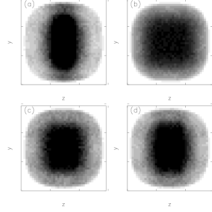
Figure 16: (a) Gray scale plot of the distribution $f(x,y)$ generated for a localised ensemble of $6400$ initial conditions with $E=10$ evolved without perturbations in the potential (2) with $a=b=1$, with data recorded at intervals ${\delta}t=1$ for $64<t<128$. (b) The invariant distribution associated with a much longer time integration. (c) The same as (a) but allowing for periodic driving with ${\Omega}=1$ and $A=10^{-1.5}$. (d) The same as (c) but with $A=10^{-2.5}$.

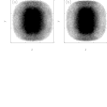
Figure 17: (a) Gray scale plot of the distribution $f(x,y)$ generated for the same initial ensembles as in the preceding figure, now allowing for additive white noise with ${\Theta}=10$ and ${\eta}=10^{-4}$. (b) The same as (a) but with ${\eta}=10^{-6}$.

What this could imply for the visual appearance of a galaxy is illustrated in FIGS. 16 and 17, which exhibits grey scale plots generated from the same orbit integrations. The first panel in FIG. 16 exhibits the distribution $f(z,y)$ for an unperturbed integration, generated from data recorded at intervals ${\delta}t=1$ for $64{\;}{\leq}{\;}t{\;}{\leq}{\;}128$. The obvious point is that, even though the potential exhibits cubic symmetry, the orbits are more localised in the $z$-direction than in the $y$- (or $x-$) direction. The second panel exhibits $f(z,y)$ much later on, namely for $896{\;}{\leq}{\;}t{\;}{\leq}{\;}1024$, by which time the distribution has become much more symmetric. The lower panels, again generated for $64{\;}{\leq}{\;}t{\;}{\leq}{\;}128$, exhibit $f(z,y)$ for the same initial ensemble now evolved in the presence of periodic driving with two different frequencies. FIGS. 17 (a) and (b) exhibit analogous plots generated from noisy integrations, It is evident in each case that, because of the perturbations, the distribution is more nearly symmetric than was the case for an integration with no perturbations.

5 DISCUSSION

To assess the importance of all this for galactic dynamics, one must determine the extent to which orbit trapping and slow phase space diffusion, seemingly generic phenomena for nonintegrable potentials that admit a coexistence of both regular and chaotic orbits, are present in the cuspy, traxial potentials which appear to characterise many galaxies.

As a concrete example, consider the maximally triaxial ${\gamma}=1$ Dehnen potential (Merritt and Fridman 1996), which is generated self-consistently from the mass density

$${\rho}(m)={(3-{\gamma})M\over 4{\pi}abc}m^{-{\gamma}}(1+m)^{-(4-{\gamma})}$$ (16)

with

$$m^{2}={x^{2}\over a^{2}}+{y^{2}\over b^{2}}+{z^{2}\over c^{2}},$$ (17)

for ${\gamma}=1$, $c/a=1/2$, and $(a^{2}-b^{2})/(a^{2}-c^{2})=1/2$. For each of twenty different energies, some $300-400$ well separated initial conditions were identified, all corresponding to chaotic orbits. [These were the chaotic initial conditions used to generate Siopis’s (1998) library of orbits for the construction of equilibria using Schwarzschild’s (1979) method.] Each initial conditions was integrated for a time $2048t_{D}$, with ${\chi}(t)$ recorded at intervals ${\delta}t=1$. As for the computations described in Section 2, the resulting data were then partitioned into segments of various length $t$ and the dispersion ${\sigma}_{\chi}$ was studied as a function of $t$.

The principal conclusion from this analysis is that, at least for this potential, unperturbed phase space transport always proceeds very slowly. For relatively high energies, the observed distributions of short time Lyapunov exponents are similar to what is found for the potential (2) for choices of the parameters $a$ and $b$ and the energy $E$ for which “stickiness” is a frequent occurence. Moreover, as for that potential, the time scale on which details wash out and the dispersion begins to decay as $t^{-1/2}$ is of order $1000t_{D}$. However, for the lowest energies, where chaotic orbits pass very close to the central cusp, phase space transport appears to proceed even more slowly! Distributions of short time Lyapunov exponents tend to exhibit considerable structure, even for comparatively long times. Indeed, even after $2048t_{D}$ there is no suggestion that the distinctions between different populations have been erased. This is illustrated in FIG. 18, which exhibits ${\sigma}_{\chi}(t)$ for the two highest and lowest energies used by Merritt & Fridman (1996) in their construction of Schwarzschild equilibria.

The obvious inference is that, at least for this triaxial Dehnen potential, unperturbed chaotic orbits often diffuse through phase space only very slowly, especially at low energies. The two obvious questions then are: (i) is this result generic for cuspy triaxial potentials, or just an accident for this specific potential, and (ii) to what extent can low amplitude friction and noise accelerate even this very slow phase space transport? Both these questions are currently being addressed (Siopis & Kandrup 1999).

Figure 1: $N[{\chi}(t)]$, the distribution of short time Lyapunov exponents for a collection of chaotic orbits with energy $E=6$ evolved in the potential (2) with $a=3$ and $b=-1$, computed as a function of the sampling time $t$. (a) $t=1$. (b) $t=4$. (c) $t=16$. (d) $t=64$. (e) $t=256$. (f) $t=1024$. (g) $t=4096$ (h) $t=16384$.

Figure 2: $N[{\chi}(t)]$, the distribution of short time Lyapunov exponents for a collection of chaotic orbits with energy $E=6$ evolved in the potential (2) with $a=b=1$, computed as a function of the sampling time $t$. (a) $t=1$. (b) $t=4$. (c) $t=16$. (d) $t=64$. (e) $t=256$. (f) $t=1024$. (g) $t=4096$ (h) $t=16384$.

Figure 3: (a) The dispersion ${\sigma}_{\chi}(t)$, plotted as a function of the sampling time $t$, for a collection of chaotic orbits with energy $E=4$ evolved in the potential (2) with $a=b=1$. The dashed line corresponds to a $t^{-1/2}$ dependence. (b) The same for chaotic orbits with $E=6$ and $a=b=1$. (c) The same for chaotic orbits with $E=6$ and $a=3$ and $b=-1$. (d) The same for chaotic orbits with $E=10$ and $a=3$ and $b=-1$.

Figure 4: Visual representations of the orbit used to compute Fig. 4. The left hand panels exhibit data for times $15700<t<16212$. The right hand panels exhibit data for $15700<t<16724$, an interval twice as long.

Figure 5: A coarse-grained estimate of the largest short Lyapunov exponent ${\chi}$, generated for a chaotic orbit in the potential (3) with $E=4$ and $a=b=1$. The coarse-graining was effected by computing ${\chi}(t)$ for successive intervals ${\delta}t=1$, and performing a box-car average over $256$ adjacent intervals.

Figure 6: The analogue of Fig. 5 for an initial condition with $E=10$, in this case integrated in the potential (3) with $a=1.6$ and $b=0.4$. In this case, the integration times for the left and right hand panels are ${\Delta}t=400$ and ${\Delta}t=800$.

Figure 7: $N(t)$, the fraction of the orbits from a 1000 orbit ensemble not yet having escaped at time $t$, computed for an initial condition with $E=10.0$ evolved in the dihedral potential with $a=0.4$ and $b=1.6$ in the presence of periodic driving with $5{\;}{\leq}{\;}{\omega}{\;}{\leq}{\;}6$ and variable amplitude $A=10^{-2}$ (solid line), $A=10^{-3}$ (dashed), $A=10^{-4}$ (dot-dashed), $A=10^{-5}$ (triple-dot-dashed), and $A=10^{-7}$ (dotted).

Figure 8: (a) $T(0.01)$, the first escape time for 1% of an ensemble of 2000 integrations of the initial condition in Fig. 6, driven with frequencies $2{\;}{\leq}{\;}{\omega}{\;}{\leq}{\;}3$ and variable amplitude. (b) The same for $5{\;}{\leq}{\;}{\omega}{\;}{\leq}{\;}6$. (c) $T(0.01)$ for the same initial condition, now plotted as a function of ${\omega}$ for fixed amplitude $A=10^{-3}$. (d) $T(0.01)$ plotted as a function of ${\rm log}\,{\omega}$.

Figure 9: $N(t)$, the fraction of the orbits from a 1000 orbit ensemble not yet having escaped at time $t$, computed for an initial condition with $E=10.0$ evolved in the dihedral potential with $a=0.4$ and $b=1.6$ in the presence of additive white noise with ${\Theta}=10.0$ and variable ${\eta}=10^{-3}$ (solid line), ${\eta}=10^{-4}$ (broad dashes), ${\eta}=10^{-4.5}$ (short dashes), ${\eta}=10^{-5}$ (dot-dashed), ${\eta}=10^{-5.5}$ (triple-dot-dashed), and ${\eta}=10^{-8}$ (dotted).

Figure 10: (a) $T(0.01)$, the first escape time for 1% of an ensemble of 2000 integrations of the initial condition in Fig. 6, perturbed by additive white noise with ${\Theta}=10.0$ and variable ${\eta}$. (b) The same for a different initial condition.

Figure 11: $N(t)$, the fraction of the orbits from a 1000 orbit ensemble not yet having escaped at time $t$, computed for an initial condition with $E=10.0$ evolved in the dihedral potential with $a=0.4$ and $b=1.6$ in the presence of different white noises with ${\Theta}=10.0$ and ${\eta}_{0}=10^{-4}$. The solid curve represents additive white noise and friction with constant ${\eta}$. The dot-dashed, triple-dot-dashed, and dotted curves represent, respectively, friction and noise with ${\eta}{\;}{\propto}{\;}v$, $v^{2}$ and $v^{3}$. The dashed curve represents additive white noise but vanishing friction.

Figure 12: $N(t)$, the fraction of the orbits from a $4800$ orbit ensemble not yet having escaped at time $t$, computed for the initial condition exhibited in Fig. 9, allowing for friction and colored noise given by eq. (5.2) with ${\Theta}=10$, ${\eta}=10^{-5}$, and either white noise (triple-dot-dashed) or variable ${\alpha}=2.0$ (dot-dashed), ${\alpha}=0.2$ (broad dashes), and ${\alpha}=0.02$ (solid).

Figure 13: (a) $T(0.01)$, the first escape time for 1% of an ensemble of $4800$ integrations, computed for the initial condition used to generate Fig. 9, plotted as a function of ${\rm log}\,{\eta}$ for fixed ${\alpha}=2.0$ for the stochastic processes defined by (5.1) (diamonds) and (5.2) (triangles), allowing for both friction and noise. (b) $T(0.01)$ for the same initial condition, plotted as a function of ${\rm log}\,{\alpha}$ for fixed ${\eta}=10^{-5}$, for the stochastic processes (5.1) (diamonds) and (5.2) (triangles), again allowing for both friction and noise. The dashed line represents the asymptotic value for white noise $({\alpha}\to\infty)$. (c) The same as (a), albeit for a different initial condition and with ${\alpha}=0.2$. (d) The same as (b), albeit for the initial condition in (c) and with ${\eta}=10^{-7}$. as (a) and (b) for another initial condition.

Figure 14: (a) The dispersion ${\sigma}_{x}$ generated for a localised ensemble of $6400$ initial conditions with $E=10$ evolved without perturbations in the potential (2) with $a=1=1$. (b) The dispersion ${\sigma}_{z}$ for the same ensemble. (c) ${\sigma}_{x}$ for the same ensemble, now allowing for periodic driving with ${\Omega}=1$ and $A=10^{-1.5}$. (d) ${\sigma}_{x}$ for the same ensemble, allowing for periodic driving with ${\Omega}=1$ and $A=10^{-1.5}$.

Figure 15: (a) The dispersion ${\sigma}_{x}$ generated for the same ensemble evolved in the presence of friction and additive white noise with ${\Theta}=10$ and ${\eta}=10^{-4}$. (b) The dispersion ${\sigma}_{z}$ for the same computation. (c) The same as (a) but with ${\eta}=10^{-6}$. (d) The same as (b) but with ${\eta}=10^{-6}$.

Figure 18: The analogue of Fig. 3 for chaotic orbits in the maximally traxial ${\gamma}=1$ Dehnen potential. The upper panels are for the two highest energies used by Merritt & Fridman (1996). The lower panels are for the two lowest energies.

References

- [1] Alexander, F. J., Habib, S. 1993, Phys. Rev. Lett. 71, 955
- [2] Armbruster, D., Guckenheimer, J., Kim, S. 1989. Phys. Lett. A 140, 416
- [3] Arnold, V. I. 1964, Russ. Math. Surveys 18, 85
- [4] Athanassoula, E., Bienyamé, O., Martinet, L., Pfenniger, D., 1983, A&A 127, 349
- [5] Binney, J. 1978, Comments Astrophys. 8, 27
- [6] Chandrasekhar, S. 1941, ApJ 94, 511
- [7] Chandrasekhar, S. 1943a, ApJ 97, 255
- [8] Chandrasekhar, S. 1943b, Rev. Mod. Phys. 15, 1
- [9] Contopoulos, G. 1971. AJ 76, 147
- [10] Fermi, E. 1949, Phys. Rev. 75, 1169
- [11] Grassberger, P., Badii, R., Politi, A. 1988, J. Stat. Phys. 51, 135
- [12] Greiner, A., Strittmatter, W., Honerkamp, J. 1988, J. Stat. Phys. 51, 95
- [13] Habib, S., Kandrup, H. E., Mahon, M. E., 1996, Phys. Rev. E 53, 5473
- [14] Habib, S., Kandrup, H. E., Mahon, M. E., 1997, ApJ 480, 155
- [15] Habib, S., Ryne, R. 1995, Phys. Rev. Lett. 74, 70
- [16] Honerkamp, J., 1994, Stochastic Dynamical Systems. VCH Publishers, New York.
- [17] Kandrup, H. E. 1998, MNRAS 301, 960
- [18] Kandrup, H. E., Eckstein, B. L., Bradley, B. O. 1997, A& A 320, 65
- [19] Kandrup, H. E., Mahon, M. E., 1994a, Phys. Rev. E 49, 3735
- [20] Kandrup, H. E., Mahon, M. E., 1994b, A&A 290, 762
- [21] Kormendy, J., Bender, R. 1996, ApJL 464, 119
- [22] Lindenberg, K., Seshadri, V., 1981, Physica 109 A, 481
- [23] Lichtenberg, A. J., Lieberman, M. A. 1992, Regular and Chaotic Dynamics. Springer, Berlin
- [24] Lieberman, M. A., Lichtenberg, A. J., 1972, Phys. Rev. A 5, 1852
- [25] Lynden-Bell, D. 1967, MNRAS 136, 101
- [26] Machta, J., Zwanzig, R. 1983, Phys. Rev. Lett. 50, 1959
- [27] Mahon, M. E., Abernathy, R. A., Bradley, B. O., Kandrup H. E., 1995, MNRAS 275, 443
- [28] Merritt, D. 1996, Science 241, 337
- [29] Merritt, D. 1999 PASP 111, 129
- [30] Merritt, D., Fridman, T. 1996, ApJ 460, 136
- [31] Merritt, D., Valluri, M. 1996, ApJ 471, 82
- [32] Nekhoroshev, N. N. 1977, Usp. Mat. Nauk USSR 32, 6
- [33] Percival, I. 1979, in Month, M., Herrara, J. C., eds. Nonlinear Dynamics and the Beam-Beam Interaction, AIP Conf. Proc. 57, p. 302
- [34] Pogorelov, I. V., Kandrup, H. E. 1999. Phys. Rev. E, in press
- [35] Schwarzschild, M. 1979, ApJ 232, 236
- [36] Siopis, C. 1998, University of Florida Ph. D. dissertation
- [37] Siopis, C., Kandrup, H. E. 1999, in preparation
- [38] Sridhar, S., Touma, J. 1996, MNRAS 287, L1
- [39] Sridhar, S., Touma, J. 1997, MNRAS 292, 657
- [40] van Kampen, N. G. 1981, Stochastic Processes in Physics and Chemistry. North Holland, Amsterdam
- [41] Wozniak, H., in Gurzadyan, V. G., Pfenniger, D., eds. Ergodic Concepts in Stellar Dynamics. Springer, Berlin