Effects of Jet-like Explosion in SN 1987A

Abstract

We study the effects of jet-like explosion in SN 1987A. Calculations of the explosive nucleosynthesis and the matter mixing in a jet-like explosion are performed and their results are compared with the observations of SN 1987A. It is shown that the jet-like explosion model is favored because the radioactive nuclei $\rm{}^{44}Ti$ is produced in a sufficient amount to explain the observed luminosity at 3600 days after the explosion. This is because the active alpha-rich freezeout takes place behind the strong shock wave in the polar region. It is also shown that the observed line profiles of $\rm Fe[II]$ are well reproduced by the jet-like explosion model. In particular, the fast moving component travelling at (3000-4000) km/s is well reproduced, which has not been reproduced by the spherical explosion models. Moreover, we conclude that the favored degree of a jet-like explosion to explain the tail of the light curve is consistent with the one favored in the calculation of the matter mixing. The concluded ratio of the velocity along to the polar axis relative to that in the equatorial plane at the Si/Fe interface is $\sim 2:1$. This conclusion will give good constraints on the calculations of the dynamics of the collapse-driven supernova. We also found that the required amplitude for the initial velocity fluctuations as a seed of the matter mixing is $\sim 30\%$. This result supports that the origin of the fluctuations is the dynamics of the core collapse rather than the convection in the progenitor. The asymmetry of the observed line profiles of $\rm Fe[II]$ can be explained when the assumption of the equatorial symmetry of the system is removed, which can be caused by the asymmetry of the jet-like explosion with respect to the equatorial plane. In the case of SN 1987A, the jet on the north pole has to be stronger than that on the south pole in order to reproduce the observed asymmetric line profiles. Such an asymmetry may also be the origin of the pulsar kick. When we believe some theories that cause such an asymmetric explosion, the proto-neutron star born in SN 1987A will be moving in the southern part of the remnant.

Department of Physics, School of Science, the University of Tokyo, 7-3-1 Hongo, Bunkyoku, Tokyo 113, Japan

1 INTRODUCTION

The collapse-driven supernovae have been playing a great important role in the history of the chemical evolution in the universe. Almost all of astronomers believe that the universe was born once upon a time (e.g. Weinberg (1972)). Then the baryon number is violated in the space (e.g. through the electroweak phase transition; Kuzmin et al. (1985)). Light nuclei such as Li, Be, and B are synthesized by the big-bang nucleosynthesis (e.g. Walker et al. (1991)). Finally, heavy nuclei are synthesized in massive stars and ejected into the space through the supernova explosions (e.g. Arnett (1996)).

In particular, the collapse-driven supernovae have been making a great contribution to the enrichment of heavy elements in the universe. $\alpha$ nuclei, such as O, Si, and S are mainly synthesized in the collapse-driven supernovae (Hashimoto (1995); Timmes et al. (1995)). Their contribution to the enrichment of heavy elements in our galaxy is about ten times higher than that of Type Ia supernovae (Tsujimoto et al. (1995)). The chemical composition of the intracluster medium can be also explained well by the abundance pattern of the collapse-driven supernovae (Loewenstein & Mushotzky (1996); Nagataki & Sato 1998a ). More advanced discussions will be presented when its chemical composition can be determined more precisely by advanced numerical calculations and observations. This proves the importance of studying the phenomena of the collapse-driven supernovae.

In the present circumstances, the mechanism of the collapse-driven supernovae can not be understood absolutely (e.g. Bethe (1990)). Many astronomers believe that the outline of the scenario for a progenitor to explode has already been understood. In fact, Wilson (1985) reported that a successful explosion can be attained when the effect of the ’delayed’ neutrino heating is taken into consideration. This is the most promising mechanism of the delayed explosion. However, the explosion energy inferred from his simulation ($\sim 0.4\times 10^{51}$ ergs) seems to be smaller than the observed one in SN 1987A ($\sim 1\times 10^{51}$ ergs; Woosley (1988); Shigeyama et al. (1988)). Generally speaking, it is said that the roles of many important phenomena and processes other than the neutrino heating have to be investigated in order to obtain a more realistic explosion model. For example, the effects of convection and the neutrino opacities that regulate the driving neutrino luminosities are investigated in order to enhance the explosion energy in their models (Herant et al. (1994); Bethe (1995); Burrows & Hayes (1995); Janka & M$\rm\ddot{u}$ller (1996)).

Other than the effects mentioned above, some researchers investigate the effects of rotation of a progenitor (LeBlanc & Wilson (1970); M$\rm\ddot{u}$ller et al. (1980); Tohline et al. (1980); M$\rm\ddot{u}$ller & Hillebrandt (1981); Bodenheimer & Woosley (1983); Symbalisty (1984); M$\rm\ddot{o}$nchmeyer $\&$ M$\rm\ddot{u}$ller (1989); Finn & Evans (1990); Yamada & Sato (1994)). They reported that the system becomes globally asymmetric by means of its effects. In particular, some researchers reported that a strong shock wave propagates along to the rotational axis when an axial symmetry of the system is assumed. Yamada & Sato (1994) showed clearly that a shock wave becomes jet-like with an increase of the angular momentum in the iron core. The qualitative explanation is given as follows: the iron core in the equatorial plane can not sufficiently collapse due to the centrifugal force. As a result, the gravitational energy can not be released well and the strength of the shock wave is reduced. On the other hand, the iron core around the polar region collapses sufficiently and generates a strong shock wave. Moreover, Shimizu, Yamada, & Sato (1994) showed that neutrino heating from an oblate proto-neutron star, whose form is the consequence of rotation (Tohline et al. (1980); M$\rm\ddot{u}$ller & Hillebrandt (1981)), also helps to cause a jet-like explosion. An magnetized rotating proto-neutron star can also generate a jet-like explosion because of the magnetic buoyancy (LeBlanc & Wilson (1970); Symbalisty (1984)).

The existence of asymmetry in a collapse-driven supernova is also supported by the observations (e.g. Burrows (1998)). For example, some observations of SN 1987A suggest the asymmetry of the explosion. The clearest is the speckle image of the expanding envelope with high angular resolution (Papaliolis et al. (1989)), in which an oblate shape with an axis ratio of $\sim 1.2-1.5$ was shown. Similar results were also obtained from the measurement of the linear polarization of the scattered light from the envelope (Cropper et al. (1988)). It is noted that no net linear polarization is induced from a spherically symmetric scattering surface. Assuming that its shape is an oblate or prolate spheroid, one finds that the observed linear polarization corresponds to an axis ratio of $\sim 1.2$ for SN 1987A. Moreover, the direction of the polarization is also found to be close to that of the elongation of the SN debris (Nisenson & Papaliolios (1999)). There is also growing evidence that the polarization is a rather common phenomenon among the collapse-driven supernovae (M$\acute{e}$ndez et al. (1988); Wang et al. (1996)).

However, it is noted that the propagation of a jet-like shock wave in the only iron core is solved in the numerical calculations mentioned above. This is because the most difficult problem with the supernova dynamics is the penetration of the shock wave through the iron core, where the photo-dissociation of the nuclei occurs and much of the thermal energy is wasted for the dissociation. It is also noted that much more CPU time is necessary to follow the whole explosion. Moreover, as stated above, almost all of simulations concerned with the dynamics of the explosion resulted in failure. So, when a numerical simulation is performed for the phenomena that occur in the outer layers, such as the explosive nucleosynthesis, an initial shock wave is assumed at the Si/Fe interface and its propagation is followed. It is also noted that a shock wave has been assumed to be spherically symmetric in almost all of precise calculations concerned with explosive nucleosynthesis in these layers (Hashimoto (1995); Woosley & Weaver (1995); Thielemann et al. (1996)). So, we want to emphasize it important to calculate the explosive nucleosynthesis assuming a jet-like explosion and to compare its results with the observations. If the jet-like explosion model can explain the observations better than the spherical ones, it means that a jet-like explosion is supported by the observations. At the same time, if a proper degree of the jet-like explosion can be determined from the observations, it means that we can make a constraint on the degree by the observations. It will be a very important information on the dynamics of the collapse-driven supernovae.

There is only one calculation concerned with the explosive nucleosynthesis behind a jet-like shock wave (Nagataki et al. (1997)). It is reported that the radioactive element, $\rm{}^{44}Ti$, can be synthesized more in a jet-like explosion model because the active alpha-rich freezeout takes place behind the strong shock wave. This result was compared with the observations of SN 1987A, which gives various precise data because of its vicinity and youth. They found that $\rm{}^{44}Ti$ in the jet-like explosion model is synthesized in a sufficient amount to explain its bolometric luminosity around $\sim 1400$ days after the explosion. Recently, its luminosity at $\sim 3600$ days after the explosion was reported (Soderberg et al. (1999)). Since the half-life of $\rm{}^{44}Ti$ is longer than those of other main radioactive nuclei such as $\rm{}^{56}Co$ and $\rm{}^{57}Co$, the recent data is more useful to extract the contribution of $\rm{}^{44}Ti$ and determine its amount. In this paper, the proper degree of the jet-like explosion in SN 1987A is estimated using this observation. At the same time, its degree can be estimated using an independent observation, the line profile of Fe[II] (Nagataki et al. 1998b ). We will present its further discussions in this paper. Finally, we will conclude the proper degree of jet-like explosion in SN 1987A in order to explain these observations. The concluded ratio of the velocity along to the polar axis relative to that in the equatorial plane at the Si/Fe interface is $\sim 2:1$. Discussions about the meaning of this conclusion are also presented.

In section 2, we show our method of calculation. We consider the problem with the explosive nucleosynthesis in section 3. Matter mixing is discussed in section 4. Summary is presented in section 5.

2 METHOD OF CALCULATION

In this section, we present the method of the simulations in this study. It is true that there are some assumptions and simplifications in our simulations. There are two reasons for such treatments. One is that the supernova dynamics can not be followed from the onset of the gravitational collapse, as mentioned in section 1. We have to start a simulation assuming an initial shock wave at the Si/Fe interface. The other is that this is the first step for the calculation of the explosive nucleosynthesis solving a multi-dimensional hydrodynamics in a collapse-driven supernova. We note that there has been no such a simulation before Nagataki et al. (1997). We have to improve the accuracy of the simulation step by step. We explain what is assumed and simplified in the following subsections.

2.1 Hydrodynamics

2.1.1 The Scheme

We performed 2-dimensional hydrodynamic calculations. The calculated region corresponds to a quarter part of the meridian plane under the assumption of axisymmetry and equatorial symmetry. The number of meshes is $300\times 10$ (300 in the radial direction and 10 in the angular one) for the calculation of explosive nucleosynthesis and $2000\times 100$ for the matter mixing. Higher resolution is needed for the matter mixing since growth of a small initial fluctuation has to be followed. We did not perform 3-dimensional hydrodynamic calculations but 2-dimensional ones to save CPU time and memory size of the supercomputer. In fact, there is no 3-dimensional calculation with high resolution in the world for the matter mixing in a supernova ejecta. Much more CPU time and memory size beyond the capacity of presently available supercomputers are necessary in order to obtain quantitative results with 3-dimensional calculations. However, the propagation of a jet-like shock wave along with the polar axis, where the system is calculated 3-dimensionally even in a 2-dimensional calculation, is performed in this study. So dimensional effects seem to be little. The Roe scheme, which solves Riemann’s problem with high accuracy and little CPU time, is used for the calculations (Roe (1981); Yamada & Sato (1994)). So it is a good scheme for calculating the propagation of a shock wave in a star. However, an Eulerian coordinate is used for the multi-dimensional calculations. That is why we use the test particle method (Nagataki et al. (1997)) in order to obtain the informations on the time evolution of the physical quanta on the frame comoving with the matter, which are used for the calculations of the explosive nucleosynthesis. We briefly explain the test particle method. Test particles are scattered in a star and at rest at first. These move with the local velocity at their own positions after the passage of the shock wave. At each time step, temperature and density that each test particle experiences are preserved. This is the test particle method we use. See Nagataki et al. (1997) and Nagataki et al. (1998b) for more details.

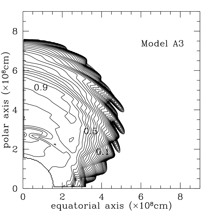
Figure 3: Contours of the mass fraction of $\rm{}^{56}Ni$ after the explosive nucleosynthesis. Contours are drawn for the initial position of the matter in the progenitor. The inner boundary at $r\sim 1.8\times 10^{8}$ cm means the Si/Fe interface. Left: the result for the model S1. The maximum value of the mass fraction of $\rm{}^{56}Ni$ is $9.3\times 10^{-1}$. The regions where the mass fraction of $\rm{}^{56}Ni$ becomes 0.9, 0.5, and 0.1 are noted in the figure. Right: Same as left, but for the model S1. The maximum value is $9.1\times 10^{-1}$.

We comment on the assumptions and simplifications in this study. Calculations of hydrodynamics and explosive nucleosynthesis are performed separately, since the entropy produced during the explosive nucleosynthesis is much smaller ($\sim$ a few $\%$) than that generated by the shock wave. In calculating the total yields of elements, we assume that each test particle has its own mass determined from their initial distribution so that their sum becomes the mass of the layers where these are scattered, and also assume that the nucleosynthesis occurs uniformly in each mass element. These assumptions will be justified since the movement of the test particles is not chaotic (i.e. distribution of the test particles at final time still reflects the given initial condition) even in a calculation of the matter mixing (see Figures 9 and 10) and the intervals of test particles are sufficiently narrow to investigate the contours of the chemical composition in the ejecta (see Figures 3, 4, 5, and 6).

2.1.2 Initial Conditions

We comment on the initial conditions. The initial velocity behind a shock wave is assumed to be radial and proportional to $r\times(1+\alpha\cos(2\theta))/(1+\alpha)$, where r, $\theta$, and $\alpha$ are radius, the zenith angle, and the free parameter that determines the degree of the jet-like explosion. Since the ratio of the velocity in the polar region to that in the equatorial one is $(1+\alpha)/(1-\alpha)$ : 1, more extreme jet-like shock waves are obtained as $\alpha$ gets larger. In this study, we take $\alpha=0$ for the spherical explosion and $\alpha=\frac{1}{3},\;\frac{3}{5},\;\rm and\;\frac{7}{9}$ (these values mean that the ratios of the velocity are 2:1, 4:1, and 8:1, respectively) for the jet-like ones. We name these models S1, A1, A2, and A3, respectively. We assumed that the distribution of thermal energy is same as the velocity distribution and that total thermal energy is equal to total kinetic one. The explosion energy is set to be $1\times 10^{51}\rm ergs$ and injected to the region of $(1.0-1.5)\times 10^{8}\rm cm$ (that is, at the Fe/Si interface). We notice again that the form of the initial shock wave can not be known $\it a\;priori$. That is why we take $\alpha$ as a free parameter. Its proper value is inferred from the comparison of calculations with the observed luminosity and line profiles of Fe$\rm[II]$ in SN 1987A in this study.

As for the seed of the matter mixing, we perturb only velocity field inside the shock wave when it reaches the He/H interface. For the jet-like explosion, we introduce the perturbation when the shock front in the polar region reaches the interface. We adopt the monochromatic perturbations, i.e., $\delta v\;=\;\varepsilon v(r,\theta)\cos(m\theta)$ ($m$=20; Hachicu et al (1992); Yamada & Sato (1991)). It is noted that test particle method will be more valid when we adopt the monochromatic perturbations rather than the random perturbations. This is because the movement of the test particles becomes chaotic when the random perturbations are adopted. Moreover, as the mixing width, i.e., the length of the mushroom-like ’fingers’, depends mainly on the density structure of the presupernova model and on the value of $\varepsilon$ rather than its mode (Hachicu et al (1992)), we think we can use this monochromatic perturbation method in order to estimate the degree of the matter mixing and construct the line profiles of the heavy elements. $0\%$, $5\%$, and $30\%$ are taken for the value of $\varepsilon$. The reason why we take $5\%$ and $30\%$ for the amplitudes of the perturbation is explained in subsection 4.1. Models for the initial shock wave are summarized in Table 1.

As for the progenitor of SN 1987A, Sk-69^∘202, it is thought to have had the mass $\sim 20M_{\odot}$ in the main-sequence stage (Shigeyama et al. (1988); Woosley & Weaver (1988)) and had $\sim$ (6$\pm$1)$M_{\odot}$ helium core (Woosley (1988)). In this study, the presupernova model obtained from the evolution of 6 $M_{\odot}$ helium core (Nomoto & Hashimoto (1988)) is used for the calculation of explosive nucleosynthesis. However, it is reported that this 6 $M_{\odot}$ model seems to be neutron-rich in the Si– rich layer and that $Y_{e}$ in the layer has to be changed higher to suppress the overproduction of neutron-rich nuclei (Hashimoto (1995)). This means that the range of convective mixing in the presupernova model is artificially changed (Hashimoto (1995)). This treatment is also justified when effects of the delayed explosion are taken into consideration (Thielemann et al. (1996)). The reason is as follows. The system behind the shock wave is photon-dominated and the temperature is almost determined as a function of radius, irrespective of the density. So the range where the explosive silicon burning occurs becomes wider when the matter falls toward the central compact object before the delayed explosion occurs. When we guess the location of the mass cut (the boundary between the ejecta and the central compact object) by the amount of $\rm{}^{56}Ni$ in the ejecta (this is explained in subsection 2.3), the mass cut is located at a more outer layer, where $Y_{e}$ is higher than that in the inner layer. Making $Y_{e}$ in the inner Si– rich layer higher will reflect this tendency effectively. In this study, we changed the value of $Y_{e}$ between $M=1.637M_{\odot}$ and the Si/Fe interface to that at $M=1.637M_{\odot}$ (= 0.499). As for the calculation of matter mixing, hydrogen envelope with 10.3 $M_{\odot}$ is attached on the helium core. This is because a mass loss of a few solar masses is thought to have occurred before the explosion (Saio et al. (1988)).

2.2 Nuclear Reaction Network

Since the chemical composition behind the shock wave is not in nuclear statistical equilibrium, the explosive nucleosynthesis has to be calculated using the time evolution of $(\rho,T)$ and a nuclear reaction network. $(\rho,T)$ on the frame comoving with the matter can be obtained by means of the test particle method (see subsubsection 2.1.1). The nuclear reaction network contains 250 species (see Table 2). We add some species around $\rm{}^{44}Ti$ to Hashimoto’s network that contains 242 nuclei (Hashimoto, Nomoto, & Shigeyama (1989)), since we focus mainly on its abundance in section 3. But, it turned out that the result was not changed effectively by the addition.

2.3 The Way of Determining the Mass Cut

In a collapse-driven supernova, there is a boundary between the ejecta and the central compact object. This boundary is called as a mass cut. It is a very difficult problem to determine its location (Woosley & Weaver (1995); Hashimoto (1995); Thielemann et al. (1996); Shigeyama & Tsujimoto (1998); Nakamura et al. (1999)). If the dynamics of a collapse-driven supernova can be followed from the onset of the core collapse to the final explosion, the location of the mass cut will be determined consistently by the hydrodynamic simulation. However, as stated in section 1, such a calculation has not been reported yet. Even if a location of the mass cut is determined by a hydrodynamic calculation for the explosive nucleosynthesis, it will be influenced by the initial condition, such as the initial shock wave given at the Si/Fe interface. Moreover, it is very difficult to determine its location hydrodynamically since it is sensitive not only to the explosion mechanism, but also to the presupernova structure, stellar mass, and metallicity. In fact, it is reported that total amount of $\rm{}^{56}Ni$ observed in SN 1987A is not reproduced when the location of the mass cut is determined by the hydrodynamic calculations (Woosley & Weaver (1995)).

There is another way to determine its location. Among many observations of SN 1987A, the total amount of $\rm{}^{56}Ni$ in the ejecta is one of the most reliable one. Moreover, $\rm{}^{56}Ni$ is synthesized in the Si– rich and the inner O– rich layers where the mass cut is located. So it is reasonable to determine its location so as to contain $\sim 0.07M_{\odot}$ $\rm{}^{56}Ni$ in the ejecta (Hashimoto (1995)). We take the same way in this study. However, this method is simple only for a spherical explosion model. We must extend this guiding principle for multi-dimensional calculations as follows. We assume that the larger total energy (internal energy plus kinetic energy) a test particle has, the more favorably it is ejected (Shimizu, Yamada, & Sato (1993)). Under the assumption, we first calculate the total energy of each test particle at the final stage ($\sim$ 10 s) of our calculations for the explosive nucleosynthesis and then add up the mass of $\rm{}^{56}Ni$ in a descending order of the total energy until the summed mass reaches $0.07M_{\odot}$. The rest particles are assumed to fall back to the central compact object. In this way, the location of the mass cut is inferred. We refer to this mass cut as A7. To check the dependence of our analysis on the form of the mass cut, we take another mass cut for comparison. The form of the another mass cut is set to be spherical and determined so as to contain $0.07M_{\odot}$ $\rm{}^{56}Ni$ in the ejecta. We refer to this mass cut as S7.

3 EXPLOSIVE NUCLEOSYNTHESIS IN SN 1987A

3.1 What are the Problems?

SN 1987A in the Large Magellanic Cloud has provided us with the most precise data to test the validity of numerical calculations of explosive nucleosynthesis in a collapse-driven supernova. The bolometric luminosity began to increase in a few weeks after the explosion (Catchpole et al. (1987); Hamuy et al. (1987)), which is attributed to the radioactive decays of $\rm{}^{56}Ni\rightarrow^{56}Co\rightarrow^{56}Fe$ (half-lives of $\rm{}^{56}Ni$ and $\rm{}^{56}Co$ are 5.9 and 77.1 days). Then the luminosity began to decline at a constant rate that coincides with the decay rate of $\rm{}^{56}Co$. The amount of ${}^{56}\rm Ni$ synthesized during the explosion is estimated to be $(0.07-0.076)M_{\odot}$ on the basis of the luminosity study (Shigeyama et al. (1988); Woosley & Weaver (1988)).

${}^{57}\rm Ni$ and ${}^{44}\rm Ti$ are also thought to be important heating sources to reproduce the form of the bolometric light curve. The decline rate is slowed down at $\sim 900$ days after the explosion (Suntzeff et al. (1991)), which suggests the existence of heating sources besides $\rm{}^{56}Co$. Since the half-lives of ${}^{57}\rm Co$ and ${}^{44}\rm Ti$ are longer than that of ${}^{56}\rm Co$ (half-lives of $\rm{}^{57}Ni$, $\rm{}^{57}Co$, and $\rm{}^{44}Ti$ are 35.6 hours, 272 days, and $\sim 60$ yrs), their relative contributions to the light curve are getting greater and greater. In particular, $\rm{}^{44}Ti$ will be the dominant heating source among the radioactive nuclei at late time. As stated in section 1, the bolometric luminosity at $\sim 3600$ days after the explosion was reported recently (Soderberg et al. (1999)). It should be emphasized that the luminosity hardly attenuates between 1700 and 3600 days after the explosion, which is easily explained if $\rm{}^{44}Ti$ is the dominant heating source during the period. The required amount of $\rm{}^{44}Ti$ to reproduce the luminosity is $\sim 1.5\times 10^{-4}M_{\odot}$. Further explanation about this amount is presented in the next subsection. As for the amount of $\rm{}^{57}Ni$, it can also be measured by the 122 keV line from $\rm{}^{57}Co$ decay (Clayton (1974); Kurfess et al. (1992)). X-ray light curve. It is reported that the ratio $\langle\rm^{57}Ni/^{56}Ni\rangle=\langle\rm^{57}Co/^{56}Co\rangle\equiv[\it X(\rm^{57}Ni)/\it X(\rm^{56}Ni)]/[\it X(\rm^{57}Fe)/\it X(\rm^{56}Fe)]_{\odot}$ is $1.5\pm 0.5$ (Kurfess et al. (1992)).

$\rm{}^{58}Ni$ is another important nucleus that is produced at the innermost region of the ejecta and gives informations about the location of the mass cut. From the spectroscopic observations, the ratio $\langle\rm^{58}Ni/^{56}Ni\rangle\equiv[\it X(\rm^{58}Ni)/\it X(\rm^{56}Ni)]/[\it X(\rm^{58}Ni)/\it X(\rm^{56}Fe)]_{\odot}$ is estimated to be 0.7-1.0 (Rank et al. (1988); Witterborn et al. (1989); Aitken et al. (1989); Meikle et al. (1989); Danziger et al. (1991)).

We have to reproduce these amounts mentioned above in the numerical calculations. We note that some excellent numerical calculations for the explosive nucleosynthesis in SN 1987A assuming a spherical explosion have been already reported (Hashimoto (1995); Woosley & Weaver (1995); Thielemann et al. (1996); Nagataki et al. (1997), hereafter we call them Ha95, WW95, TNH96, Na97, respectively). Their results are shown in Table 3. We first compare their results with the observations.

It is a matter of course for Ha95, TNH96, and Na97 to be able to reproduce the observed amount of $\rm{}^{56}Ni$, because the location of the mass cut is determined using this observed value (see subsection 2.3). As for WW95, its location is determined hydrodynamically and $\rm{}^{56}Ni$ is ejected more than the observed value. The calculated amounts of $\rm{}^{57}Ni$ in Ha95, TNH96, and Na97 are in the range of the observed value. The amount in WW95 seems to be smaller than the observed one. On the other hand, the amount of $\rm{}^{58}Ni$ is well reproduced in WW95, while the results of the other models seem to be larger. This may reflect the neutron richness of the progenitor that Ha95, TNH96, and Na97 used (Nomoto & Hashimoto (1988); Hashimoto (1995), see also subsubsection 2.1.2). Finally, the calculated amounts of $\rm{}^{44}Ti$ in Ha95, WW95, and Na97 are smaller than the required value. In fact, it is reported that $\rm{}^{44}Ti$ cannot be produced in a sufficient amount to explain the tail of the light curve in a wide parameter range (Woosley & Hoffman (1991)). Only TNH96 reproduces the required value very well.

As stated above, the calculated abundances of these nuclei do not converge among these models. This is because there are some differences of the input physics, such as the treatment of convection in a progenitor, nuclear reaction rates, and the way to initiate a shock wave among these models (Aufderheide et al. (1991); Nagataki et al. 1998c ). Unfortunately, the convergence has not been attained yet, although some efforts for the convergence has already started (Hoffman et al. (1998)). In the present circumstances, it is necessary to make our standpoint clear. Our standpoint in this study is as follows. We will present a consistent solution for the problems of the explosive nucleosynthesis and matter mixing. That is, it is shown in this study that more $\rm{}^{44}Ti$ is synthesized and ejected along with the degree of the jet-like explosion. So we can determine the favored degree of a jet-like explosion to explain the tail of the light curve. Next, we also show that the favored degree for the explosive nucleosynthesis is consistent with the one favored in the calculation of the matter mixing. So we conclude that this is a solution for these problems. It is noted that there has been no model that solves these problems at the same time. This is our standpoint in this study.

3.2 Required Amount of $\rm{}^{44}Ti$ in SN 1987A

In this subsection, the required amount of $\rm{}^{44}Ti$ is explained in detail. Observed bolometric luminosity (e.g. Suntzeff & Bouchet (1990); Suntzeff et al. (1991); Bouchet et al. 1991a ; Bouchet et al. 1991b ; Suntzeff et al. (1992)) is shown in Figure 1. The amount of $\rm{}^{56}Ni$ is determined by the luminosity around (600 – 900) days after the explosion. The luminosity at $\sim 3600$ days after the explosion (Soderberg et al. (1999)) is also plotted in the figure. It is quite apparent that the decline rate becomes smaller and smaller along with time. In particular, we can find that the luminosity hardly attenuates between 1700 and 3600 days after the explosion. This feature can be explained if $\rm{}^{44}Ti$ becomes the dominant isotope after $\sim$ 1700 days (Kozma (1999)).

Before we continue to further discussion, we must comment on the discrepancy between the observations of CTIO (Cerro Tololo Inter-American Observatory) and ESO (European Southern Observatory) around (1000 – 1200) days after the explosion. Mochizuki et al. (1998, 1999a, 1999b) obtained the required amount of $\rm{}^{44}Ti$ using the observations of CTIO and HST at $\sim 3600$ days. In their study, they try to give an unified explanation for the observations CTIO and HST. That is, the bolometric luminosity evolution deduced from the observations of CTIO and HST is reproduced in their light curve models. We use their result in this study. As for the observations of ESO, it seems to be too difficult to explain such a high luminosity around (1000 – 1200) days because the amount of $\rm{}^{57}Ni$ is limited by the X-ray observation (Kurfess et al. (1992)) and numerical calculations (Hashimoto (1995); Woosley & Weaver (1995); Thielemann et al. (1996)). It is also shown that such a large amount of $\rm{}^{57}Ni$ to reproduce the observations of ESO can not be synthesized in this study.

Mochizuki et al. (1998, 1999a) obtained the required amount of $\rm{}^{44}Ti$ as a function of its half-life using the Monte Carlo simulation method (Kumagai et al. (1991); Kumagai et al. (1993)). Their theoretical light curves (Mochizuki et al. 1999a ) are also shown in Figure 1. Solid curves are the total bolometric luminosities (half-life of $\rm{}^{44}Ti$ is assumed to be 40 and 70 yrs). Relative contributions of $\rm{}^{56}Co$, $\rm{}^{57}Co$, and $\rm{}^{44}Ti$ are also shown in the figure. The amount of $\rm{}^{56}Co$ is assumed to be 0.073$M_{\odot}$. $\langle\rm^{57}Co/^{56}Co\rangle$ is set to be 1.7. $\langle\rm^{44}Ti/^{56}Ni\rangle\equiv[\it X(\rm^{44}Ti)/\it X(\rm^{56}Ni)]/[\it X(\rm^{44}Ca)/\it X(\rm^{56}Fe)]_{\odot}$ is assumed to be 1.0. We can find $\rm{}^{44}Ti$ becomes the dominant heating source among the radioactive nuclei at late time ($\geq 1600$ days after the explosion).

The required amount of $\rm{}^{44}Ti$ in SN 1987A depends on its half-life since its decay rate means the rate of energy release from the nuclei. This proves the importance to verify the value of its half-life. Historically speaking, there was a large spread in the published values for its half-life. Its upper limit obtained by experiments is $\tau=66.6$ yrs (Alburger & Harbottle (1990)), while its lower limit is $\tau=39$ yrs (Meissner (1996)). However, in spite of the difficulty in determining the half-life of the long-lived nuclei, recent experiments give a converged value, $\tau\sim 60$ yrs. For example, Ahmad et al. (1998), G$\rm\ddot{o}$rres et al. (1998), and Norman et al. (1998) reported it to be 59.0, 60.3, and 62 yrs, respectively. This is because the skills of the experiments in reducing the systematic uncertainties gain (G$\rm\ddot{o}$rres et al. (1998)). Mochizuki et al. (1998, 1999a) obtained the required amount of $\rm{}^{44}Ti$ as a function of its half-life using the Monte Carlo simulation method (Kumagai et al. (1991); Kumagai et al. (1993)).

There are other approaches to determine the amount of $\rm{}^{44}Ti$ in SN 1987A. One of them is to observe and model the different broad bands. Since the bolometric corrections are not easy, this method may be a better one (Kozma (1999)). Kozma (1999) reproduced the light curves for the B and V bands up to 4000 days for SN 1987A and reported that the required amount of $\rm{}^{44}Ti$ is in the range (1.5$\pm$1.0)$\times 10^{-4}M_{\odot}$. In her analysis, the observations from Suntzeff & Bouchet (1990), Suntzeff et al. (1991), and HST data (Soderberg et al. (1999)) are used. As for the half-life of $\rm{}^{44}Ti$, 54 yrs is adopted in her analysis (C.Kozma, private communication). Fortunately, the result in her analysis is consistent with the result of Mochizuki et al. (1998, 1999a).

Still another method to estimate the amount of $\rm{}^{44}Ti$ is to observe and model individual line fluxes. Borkowski et al. (1997) and Lundqvist et al. (1999) estimated the required amount of $\rm{}^{44}Ti$ in SN 1987A using Infrared Space Observatory observations of the flux of Fe[II] 25.99 $\rm\mu$m line. In particular, Lundqvist et al. (1999) have checked several uncertainties in their model very precisely and given a good estimation for the amount of $\rm{}^{44}Ti$. As for the half-life of $\rm{}^{44}Ti$, 60.3 yrs is adopted in order to estimate the upper limit on the amount of $\rm{}^{44}Ti$ in their analysis (Lundqvist et al. (1999)). As a result, they reported that the upper limits are 1.5$\times 10^{-5}M_{\odot}$ (Borkowski et al. (1997)) and 1.5$\times 10^{-4}M_{\odot}$ (Lundqvist et al. (1999)), respectively. Their idea to use the line flux directly will be better than that to use the bolometric luminosity, because the bolometric corrections have to be used to estimate a bolometric magnitude (Soderberg et al. (1999)), although no line emission, such as Fe[III] 22.93$\rm\mu$m, Fe[I] 24.05$\rm\mu$m, and Fe[II] 25.99$\rm\mu$m, is reproduced in the wavelength range (23 – 27) $\rm\mu$m in their models. In particular, the lowest upper-limit on the $\rm{}^{44}Ti$ mass estimated by Borkowski et al. (1997) from their deep ISO exposure is a puzzling problem. Further modeling of those data are required to check the inconsistency among their results, those of Kozma (1999) and Mochizuki et al.(1999a).

These results mentioned above are shown in Figure 2. Data points in the figure are the required amounts of $\rm{}^{44}Ti$ as a function of its half-life, which are determined by the luminosity evolution. Trapezoidal region and filled circles are its amounts estimated by the analysis of the bolometric light curve (Mochizuki & Kumagai (1998); Mochizuki et al. 1999a ). It is noted that Mochizuki et al. (1999a) also calculated the required amount for an effectively longer half-life ($\sim$ 100 yrs). They pointed out the possibility that its half-life becomes longer if $\rm{}^{44}Ti$ is highly ionized and the decay channel of the orbital electron capture is blocked out in a supernova remnant (Mochizuki et al. 1999a ), although the temperature has to be $\sim 10000$ times higher than the observed one in SN 1987A (Haas et al. (1990)) in order to attain such a highly ionization. Open circle is that estimated by the analysis of the light curves for the B and V bands (Kozma 1999). Down arrow is the upper limit on the amount estimated by the flux of Fe[II] 25.99 $\rm\mu$m line (Lundqvist et al. (1999)). The most reliable value for its half-life is $\sim$ 60 yrs (Ahmad et al. 1998; G$\rm\ddot{o}$rres et al. 1998; Norman et al. 1998). $\tau=66.6$ yrs is the upper limit of its half-life obtained by the experiments (Alburger & Harbottle 1990). Its lower limit obtained by the experiments is $\tau=39$ yrs (Meissner 1996). Horizontal lines are results of the numerical calculations Ha95, WW95, TNH96, and Na97. WW95 represents the model T18A in their paper, since $\rm{}^{44}Ti$ is synthesized most in this model among their models in the mass range (18-21)$M_{\odot}$.

3.3 Results

Results of the calculations of the explosive nucleosynthesis are shown in this subsection. First, the contours of the mass fraction of $\rm{}^{56}Ni$ in a progenitor are shown in Figure 3. Contours are drawn for the initial position of the matter in the progenitor. The inner boundary at $r\sim 1.8\times 10^{8}$ cm means the Si/Fe interface. Left is the result for the model S1 and right is the one for A3. As can be seen from the figures, $\rm{}^{56}Ni$ is synthesized at the inner most region of the ejecta and is a good tool to determine the location of the mass cut (see subsection 2.3). It is also noted that $\rm{}^{56}Ni$ is synthesized only in the polar region in the model A3. This is because the shock wave in the polar region is strong and temperature rise high sufficiently to synthesize much of iron-group elements, while the shock wave around the equatorial plane is too weak to synthesize them. This fact has a great influence on the line profiles of Fe$\rm[II]$ in the ejecta. This is discussed in subsection 4.3 and 4.4.

Forms of the mass cut A7 are presented in Figures 4 and 5. Filled and open circles represent the test particles that will be ejected and falling back, respectively. A mass cut is defined as an interface of filled/open circles. These are plotted for their initial positions. We can find the tendency that the matter in the polar region is ejected more than that around the equatorial plane. This can be easily understood because the strong shock wave in the polar region gives more energy to the matter. These figures prove that the guiding principle to determine the location of the mass cut presented in subsection 2.3 is not so bad. This problem is also discussed in subsection 4.3 and 4.4.

Contours of the mass fraction of $\rm{}^{4}He$ and ${}^{44}\rm Ti$ after the explosive nucleosynthesis in the model A3 are drawn in Figure 6. Much of $\rm{}^{4}He$ is synthesized near the polar axis for the jet-like explosion models since a high photon to baryon ratio is achieved there. That is, photons with high energy that decompose heavy elements into light nuclei are filled in the polar region, which causes the alpha-rich freezeout (Thielemann et al. (1996); Nagataki et al. (1997)). Since $\rm{}^{44}Ti$ is produced through this process (The et al. (1998)), we can find the correlation between the contours of $\rm{}^{44}Ti$ and $\rm{}^{4}He$.

Calculated masses of $\rm{}^{44}Ti$ by the S1, A1, and A2 models are shown in Figure 7. We can see the tendency that the synthesized mass of $\rm{}^{44}Ti$ becomes larger along with the degree of the jet-like explosion. The reason for it is mentioned above. This tendency does not depend on the form of the mass cut (see Table 4). It is noted that the model A1 is a good one to explain the amount of $\rm{}^{44}Ti$ in SN 1987A. Additionally, even if the effective half-life of $\rm{}^{44}Ti$ is longer than that in a laboratory (Mochizuki et al. 1999a ), the jet-like explosion model can meet the requirement.

As for the amounts of $\rm{}^{57}Ni$ and $\rm{}^{58}Ni$, calculated amounts of these nuclei are summarized in Table 4. The calculated ratios of $\rm{}^{57}Ni/^{56}Ni$ are in agreement with the observed ratio, while the calculated ratios of $\rm{}^{58}Ni/^{56}Ni$ seem to be a little higher than the observed value. Since these ratios does not sensitive to the form of the initial shock wave and of the mass cut, these ratios may depend mainly on the progenitor model (Nagataki et al. 1998c ).

3.4 Discussion on the Explosive Nucleosynthesis

A lot of discussions have already been presented in the previous subsections. Additional comments are presented in this subsection. We have shown that $\rm{}^{44}Ti$ can be synthesized in a sufficiently amount to explain the observed luminosity in SN 1987A around 3600 days after the explosion, when a jet-like explosion is assumed. In particular, it is shown that the model A1 is a good one to explain the observed luminosity. There are other candidates that may explain the luminosity. One is a pulsar activity (Kumagai et al. (1993)) and the other is the freezeout effect (Fransson & Kozma (1993)). The freezeout effect means that the time scale of the recombination of the plasma can not be ignored and the assumption of the instantaneous energy input due to the recombination breaks down. We think that the pulsar activity is a promising candidate, although a pulsar has not been found in SN 1987A yet and its activity has not been measured. The freezeout effect is also interesting one, although there are uncertainties and difficulties in making a model for the structure of the ejecta (Fransson & Kozma (1993)). Moreover, it is reported that this freeze-out effect becomes less important as $\rm{}^{44}Ti$ starts to dominate (Lundqvist et al. (1999)). The contribution and amount of $\rm{}^{44}Ti$ will be determined clearly when the ejecta becomes optically thin and $\gamma$-ray line is detected directly, although it will take $\sim 100$ yrs.

It is also noted that $\gamma$-ray line from the decay of $\rm{}^{44}Ti$ has been detected in Cassiopeia A, which is famous for the asymmetric form of the remnant. The inferred abundance ratio of $\rm{}^{44}Ti$ relative to $\rm{}^{56}Ni$ is quite high, as a jet-like explosion model predicts (Nagataki et al. 1998d ).

Such a high entropy condition caused by a jet-like explosion will be also good for the synthesis of the rapid-process nuclei in the iron core (Woosley et al. (1994); McLaughlin et al. (1996)). We note that the nucleosynthesis in the iron core is not calculated in this study, although such a calculation is now underway. We will report the results in the near future. Additionally, a hypernova model (Iwamoto et al. (1998); Woosley et al. (1999)) will be also able to realize such a high entropy condition.

Finally, we emphasize again that we have found the favored degree of a jet-like explosion to explain the tail of the light curve. In the next section, we show this degree is also good for explaining the line profiles of Fe$\rm[II]$ in SN 1987A.

4 MATTER MIXING IN SN 1987A

4.1 What are the Problems?

SN 1987A also provided us the apparent evidence of large-scale mixing in the ejecta for the first time. For example, the early detection of X-rays (Dotani et al (1987); Sunyaev et al (1987); Wilson et al (1988)) and $\gamma$-rays (Matz et al (1988)) from the radioactive nuclei $\rm{}^{56}Co$ reveals that a small fraction of the matter at the bottom of the ejecta was mixed up to the outer layer. It should be also noted that these early detections verified the prediction derived by Clayton (1974), which had been discussed 13 years before SN 1987A exploded. The form of the X-ray light curve during (100-700) days after the explosion is also thought to be the indirect evidence of mixing and clumping of the heavy elements (Itoh et al (1987); Kumagai et al (1988)). Moreover, the observed infrared line profiles of heavy elements, such as $\rm Fe[II]$, $\rm Ni[II]$, $\rm Ar[II]$, and $\rm Co[II]$, show that a part of them is mixed up to the fast moving (3000-4000 km/s) outer layers (Erickson et al (1988)).

At present, the growth of a fluctuation in the progenitor due to the Rayleigh-Taylor (R-T) instability is thought to be the most promising scenario for the matter mixing. Although this idea was not a new one (e.g., Falk & Arnett (1973); Chevalier (1976); Bandiera (1984)), it was necessary to perform multi-dimensional hydrodynamic calculations with a realistic stellar model including the fluctuations in order to investigate their growth quantitatively. With the improvement of the supercomputers, many people have done such calculations. They performed mainly 2-dimensional calculations of the first few hours of the explosion. As a result, they showed that the fluctuations indeed grow due to the R-T instability (Arnett et al. (1989); Hachisu et al (1990); M$\rm\ddot{u}$ller et al. (1990); Fryxell et al. (1991); M$\rm\ddot{u}$ller et al. (1991)).

However, there are some points which are still open to arguments. One problem is how and where the initial fluctuations, the seed of the matter mixing, are made in a progenitor. Also, their amplitude has not been known yet. Up to the present, two candidates have been proposed for that seed. One idea is that these fluctuations are generated by the convection during the stellar evolution. It is reported that the density fluctuation at the inner and outer boundaries of the convective O– rich layer, $\delta\rho/\rho$, becomes $\sim 5\%$ (up to $8\%$) at the beginning of the core collapse (Bazan & Arnett (1994); Bazan & Arnett (1997)). The other is that the initial fluctuations are amplified when the shock wave is formed in the iron core. It is reported that the amplitude of the fluctuations, $\delta R_{s}/R_{s}$ ($R_{s}$ is the shock radius), becomes $\sim 30\%$ in the iron core (Burrows & Hayes (1995)), even if the initial fluctuations are set to be small ($\sim 1-2\%$).

Another problem is the reproduction of the observed line profiles of heavy elements. As mentioned above, the line profiles of Fe$\rm[II]$ have shown that a small fraction of Fe is traveling at (3000-4000) km/s. On the other hand, the velocities of Fe are of order 2000 km/s at most in the numerical simulations, even if the acceleration by the energy release of the radioactive nuclei is taken into account (Herant & Benz (1991); Herant & Benz (1992)). Although they insist that pre-mixing of $\rm{}^{56}Ni$ will be necessary for the reproduction, this problem seems to be unresolved. It is also noted that $2\times 10^{51}$ ergs are required for an explosion energy in order to reproduce the fast moving component in their model. As for the grobal form of the line profiles, the observed line profiles are asymmetric with a steep edge on the redshifted side and a more gradual decline on the blueshifted side. Maximum flux density is also redshifted. This feature has not been reproduced yet by the numerical simulations.

In this section, the effects of jet-like explosion on the matter mixing are investigated. It is noted that Yamada $\&$ Sato (1991) did 2-dimensional hydrodynamic calculations assuming a jet-like explosion. They found that heavy elements could be highly accelerated in a jet-like explosion and get velocities of order of 4000km/s when the amplitude of the initial fluctuations is set to be $30\%$. However, there are some points to be improved in their calculations. For example, only one model is assumed for the calculation of the jet-like explosion. The initial velocity behind the shock wave is assumed to be proportional to $r\times\cos^{2}\theta$, where $\theta$ is the zenith angle. They did not calculate the line profiles of heavy elements, which should be compared with the observations. They also assumed that the chemical composition of the ejecta and the form of the mass cut are spherically symmetric. In this study, we improve their calculations and compare the results with the observations. Our main aim is, of course, to find the proper degree of the jet-like explosion in SN 1987A.

4.2 Line profiles of Fe$\rm[II]$

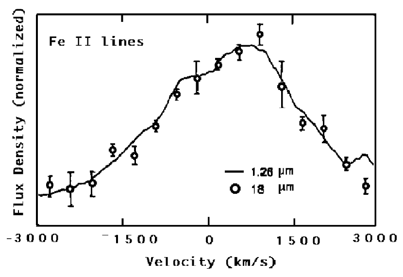
Figure 8: Observed line profiles of Fe$\rm[II]$. Left: comparison of the central portion of the 18$\rm\mu$m profile at 409 days after the explosion (Haas et al. 1990) with the 1.26 $\rm\mu$m profile at 377 days (Spyromilio et al. 1990). Positive velocity corresponds to a red-shift one. Right: Line profile of the 18$\rm\mu$m profile covering $\pm 4500$ km/s. The 1 $\sigma$ error bars are included. Adopted continuum level is indicated by dashed line.

Observed line profiles of Fe$\rm[II]$ are shown in Figure 8. A comparison of the central portion of the 18$\rm\mu$m profile at 409 days after the explosion (Haas et al. (1990)) with the 1.26 $\rm\mu$m profile at 377 days (Spyromilio et al. (1990)) is shown in the left panel. Positive velocity corresponds to a red-shift one. Although the data for the 1.26 $\rm\mu$m spectrum covers $\pm$ 3000 km/s, those for the 18$\rm\mu$m one covers $\pm$ 4500 km/s, which is shown in the right panel. Adopted continuum level is indicated by dashed line.

Several comments on the figures will be needed. First, the iron in the ejecta is mainly produced through the decays of $\rm{}^{56}Ni\rightarrow^{56}Co\rightarrow^{56}Fe$. Also, the bulk of the observed iron is Fe$\rm[II]$, as deduced from infrared transitions of Ni$\rm[I]$, Ni$\rm[II]$, and Ni$\rm[III]$ (Haas et al. (1990)). So we compare the velocity distribution of $\rm{}^{56}Ni$ in the numerical calculations with the observed line profiles of Fe$\rm[II]$. Second, we can find clearly that a small fraction of Fe is traveling at (3000-4000) km/s, which can not be reproduced by the spherical explosion models. Third, it is an important fact that the line profiles of different wave lengths share the same form of the spectrum, which shows the optical depth of the emission region is quite low. This is because the dependence of the optical depth on the wave length is quite large when the density of the system is high and the optical depth is not zero (Spyromilio et al. (1990)). Fourth, there is an apparent asymmetry of the form of the line profiles. In particular, the flux from the red-shift side is higher than that from the blue-shift side, which is contrary to the intuition. Spyromilio et al. (1990) attributed this line asymmetry primarily to emission from regions where density and/or electron temperature depart from spherical symmetry. Furthermore, Haas et al. (1990) concluded that the asymmetry results from the density inhomogeneities, rather than the temperature ones, because of the extreme temperature sensitivity of the higher excitation 1.26 $\mu$m line. Finally, Haas et al. (1990) used their radiation transfer models and concluded that the Fe$\rm[II]$ lines are partially optically thick and the missing iron is probably hidden in regions of enhanced optical depth or ’clumps’, rather than in a smooth density distribution with higher optical depths at low velocities.

In this study, we compare the velocity distribution of $\rm{}^{56}Ni$ in the numerical calculations with the observed line profiles assuming they are optically thin (Herant & Benz (1992)). This can be justified as follows. As for the reproduction of the fast moving component, it is important to show the fact that it can be produced in the jet-like explosion models. We emphasize again that it can not be reproduced by the spherical explosion models. So this fact is important, irrespective of the optical depth. As for the form of the line profiles, we use it to make a constraint on the degree of the jet-like explosion in this study. It is true that the form of the observed line profiles may change and the constraint on the degree may be also changed when the missing iron in the clumps becomes to appear. However, as shown in subsection 4.3, the calculated velocity distributions with large $\alpha$ are far from similar to the form of the observed profiles. That is why we think our conclusion in this study is not so sensitive to the presence of the missing iron. Such insensitivity will be also supported by the conclusion of Haas et al. (1990) that the missing iron is not hidden as a sphere at the center of the system but as clumps. This is because the form of the line profiles will not change so much when the missing iron in the clumps becomes to appear.

4.3 Results

Results of the calculations of the matter mixing are shown in this subsection. Density contours for the model S1b at $t$ = 5000 s after the explosion are shown in Figure 9, which tells us how the matter mixing is going on. The radius of the surface of the progenitor is 3.3 $\times 10^{12}$ cm. The shock wave can be seen at the radius $\sim 2\times 10^{12}$ cm. Hydrogen envelope is lying during (1-3.3) $\times 10^{12}$ cm. On the other hand, heavy elements, such as Ni, Fe, Si, O, and C, are packed in the layer lying $\sim 1\times 10^{12}$ cm. Additionally, a weak flow of the matter is introduced at the inner most boundary (= $10^{8}$ cm) in order to maintain the stability of the hydrodynamic calculations. The region behind the layer that contains heavy elements is filled with this artificial matter. It is noted that the total energy that the artificial matter has is much smaller than the explosion energy ($\sim 1\times 10^{51}$ ergs) and can be neglected. The growth of the fluctuations due to the R-T instability can be seen behind the shock wave. The amplitude of the fluctuations is, indeed, larger than the initial one (= $5\%$). We can find that the heavy elements are conveyed to the outer layer by the instability.

In Figure 10, we show the final positions ($t$ = 5000 s) of the test particles that meet the following conditions for the model A1c, which is concluded to be the best one in this study. The conditions are: (i) the mass fraction of $\rm{}^{56}Ni$ is larger than 0.1 and (ii) velocity is higher than 2000 km/s. As is clear from the figure, fast moving component of $\rm{}^{56}Ni$ is concentrated in the polar region, which reflects the feature of the jet-like explosion. In particular, the matter at the tip of the mushroom-like ’fingers’ in the polar region travels with a velocity higher than 3000 km/s, which is required from the observations. We have to give an additional comment. Numerical calculations in this study are performed until $t$ = 5000 s after the explosion, which are compared with the observations at $t\sim 400$ days after the explosion. This is because such a wide region can not be covered by an Eulerian coordinate used in this study. However, there are some reasons that justify our treatment. One is that the total internal energy relative to the total kinetic energy in the heavy element layer is quite small (= 0.0879), which means that the matter in this layer expands almost freely already at $t$ = 5000 s. Second, calculated velocity distributions of $\rm{}^{56}Ni$ assuming a spherical explosion in this study (see Figure 11) are similar to those in Herant et al. (1992), which are calculated until $t$ = 90 days using a smooth particle hydrodynamics code and assuming a spherical explosion (see their figure 9).

Calculated velocity distributions of $\rm{}^{56}Ni$ are shown in Figures 11 and 12. Velocity distributions are calculated assuming that the angle between the line of sight and the symmetry axis is $44^{\circ}$, which is inferred from the form of the ring around SN 1987A (Plait et al. (1995)). Asymmetric forms of the mass cut (A7) are adopted for the jet-like explosion models. As can be seen from Figure 11, fast moving component can not be reproduced in the spherical explosion models, which is consistent with other works (Herant & Benz (1991); Herant & Benz (1992)). On the other hand, fast moving component is reproduced in the jet-like explosion models when the amplitude of the initial fluctuations is set to be 30$\%$. However, the slow moving component becomes insufficient as $\alpha$ gets larger. In particular, the jet-like explosion models with no perturbation suffer from this problem.

In order to understand the cause of the problem, velocity distributions of A3a seen from $\theta=0^{\circ},44^{\circ},$ and $90^{\circ}$ are calculated. The result is shown in Figure 13. When the line of sight is parallel to the polar axis ($\theta=0^{\circ}$), the matter that contains much of $\rm{}^{56}Ni$ is travelling at a maximum speed ($\sim 2500$ km/s). On the other hand, when the system is seen from the equatorial axis, the apparent velocities of the matter are almost zero. This proves that the matter which contains much of $\rm{}^{56}Ni$ is travelling along with the polar axis. This picture can be easily explained as follows. As can be seen in Figure 3, $\rm{}^{56}Ni$ can be synthesized only in the polar region in the model A3. The synthesized $\rm{}^{56}Ni$ behind the jet-like shock wave is moving along with the polar axis. Although this feature is diluted by the presence of the fluctuations, which introduce the slow moving component, the jet-like explosion models suffer from this problem.

Next, we investigate the dependence of the results on the form of the mass cut. We can easily guess that a spherical mass cut will introduce the slow moving component around the equatorial plane, which may make up for the deficiency. The results are presented in Figures 14 and 15. We can find the enhancement of the slow moving component as we expected. However, the velocity distributions of the models A2 and A3 are still far from the observed line profiles. On the other hand, the velocity distribution of the model A1c is similar to the observed one. Furthermore, we remove the assumption of the equatorial symmetry of the system in order to reproduce the asymmetry of the observed line profiles. We found that the combination of the model A1c with the spherical mass cut (S7) and that with the asymmetric mass cut (A7) is the best one for the reproduction of the observed line profiles. This result is shown in Figure 16. This is an interesting result because it suggests the origin of a kick velocity of a pulsar (Gunn & Ostriker (1970); Lyne & Lorimer (1994)). This is discussed in the next subsection.

Finally, we verify the consistency of the conclusions on the degree of the jet-like explosion in SN 1987A, which are derived by the calculations of explosive nucleosynthesis and matter mixing. We show again the required amounts of $\rm{}^{44}Ti$ from the observed luminosity evolution are shown in Figure 17. We show the calculated amounts of $\rm{}^{44}Ti$ in the model A1 with the spherical/asymmetric mass cuts in the figure. We can find that the favored degree of a jet-like explosion to explain the tail of the light curve is consistent with the one favored in the calculation of the matter mixing. It is also noted that the combination of the model A1 with S7 and that with A7 is also the best model that reproduces the observed luminosity of SN 1987A at $\sim$ 3600 days after the explosion.

4.4 Discussion on the Matter Mixing

A lot of discussions have already been presented in the previous subsections. Additional comments are presented in this subsection. We first discuss the form of the mass cut. As stated in subsection 2.3, the mass cut is determined by a guidance principle. We also concluded that the results of the calculations on the explosive nucleosynthesis, especially on the synthesis of $\rm{}^{44}Ti$, are not sensitive to its form. However, we have to conclude that the results of the calculations on the matter mixing are sensitive. We conclude that a more spherical form than that determined by the guidance principle is required by the calculations of the matter mixing.

Next, we discuss the origin of a kick velocity of a pulsar. As shown in Figure 16, the observed line profiles are well reproduced when the assumption of the equatorial symmetry of the system is removed and the models A1c with the mass cuts A7 and S7 are combined. Such a condition will be realized when the strength of the jet generated at the north pole is different from that generated at the south pole. Some models that realize such a condition have been proposed. For example, asymmetries in density or velocity produced during the stellar evolution (Bazan & Arnett (1994); Bazan & Arnett (1997)) may cause such an asymmetric explosion (Burrows & Hayes (1996); Burrows (1996)) in which the amounts of the explosion energy in the northern and southern hemispheres are different from each other. Such an asymmetric explosion can be also caused by the effects of the asymmetric magnetic field topology on the neutrino transportation in the iron core (Lai & Qian (1998)). If we believe these theories, the proto-neutron star and the center of gravity of the ejecta are moving in opposite directions due to the conservation of the momentum. In case of SN 1987A, the jet on the northern hemisphere has to be stronger and eject more $\rm{}^{56}Ni$ than that on the southern hemisphere in order to reproduce the observed asymmetric line profiles. This is because many of the observations on the ring of SN 1987A show that the northern part of the ring is nearer to us (Michael et al. (1998)), which means that the northern part of the jet is red-shifted. In this case, the proto-neutron star born in SN 1987A is moving in the southern part of the remnant. This prediction is consistent with the one that given Fargion & Salis (1995), who discussed the effect of the precessing $\gamma$ jets on the formation of the twin rings around SN1987A. In particular, if the axial symmetry of the system is kept well, the neutron star will be running along with the polar axis. Detection of the neutron star in SN 1987A will make a strong constraint on the mechanisms of pulsar kick and jet-like explosion. Also, it is noted that the reproduced asymmetric line profile in this study is only the first step of the estimation of the effects of the asymmetric explosion. There are some points to be refined as mentioned below. First, calculations of the matter mixing and explosive nucleosynthesis have to be done with the zenith angle ranged between $0^{\circ}$ and $180^{\circ}$ so that the gradients of the physical quanta on the equatorial plane can be treated correctly (these are assumed to be zero in all of the calculations in this study because the symmetry with respect to the equatorial plane is assumed from the beginning). This treatment will be important when the explosion energy on the northern hemisphere is different from that on the southern hemisphere, as the theories mentioned above predict. Second, it is noted that the same amounts of $\rm{}^{56}Ni$ are assumed to be ejected from both hemispheres in this study, which is not self-evident in an asymmetric explosion. If the observations investigated in this study can be reproduced better by these calculations, we will be able to predict the position and velocity of the pulsar born in SN 1987A more definitely using results of such advanced calculations.

We comment on the jet-induced explosion of a collapsing star (MacFadyen & Woosley (1998); Khokhlov et al. (1999)). It is a very attractive theory because it has a possibility to explain a lot of observational facts and to be an origin of the $\gamma$-ray bursts (MacFadyen & Woosley (1998); Khokhlov et al. (1999)). When we believe the correlation between a $\gamma$-ray burst and a super(hyper)nova (Kulkarni et al. (1998); Galama et al. (1998)), such a jet-induced explosion model will be a convincing one for the $\gamma$-ray burst model. In this case, we note, a bipolar profile of iron like the one seen in Figure 13 should be observed when a $\gamma$-ray burst occurs near us, that is, in our galaxy and the Magellanic clouds. Such an observation will give a strong support to this model. However, it has to be also noted that such a strong jet-induced explosion is not allowed for the model of SN 1987A by the calculations of the explosive nucleosynthesis and the matter mixing investigated in this study. Here we introduce the recent work presented by Fryer & Heger (1999) who performed core-collapse simulations using a rotating progenitor star (Heger et al. (1999)). It should be emphasized that they calculated the evolution of a star from the beginning of the main-sequence stage including the effect of rotation. This means that the distribution of the angular momentum in the iron core in their progenitor model is not an artificial input parameter but a naturally derived outcome. As a result, they report the ratio of the escaping velocity of the matter behind the shock wave in the polar region relative to the one in the equatorial plane to be about two in the iron core. That is, their result is entirely consistent with our conclusion. We think such a moderate ’jet-like’ explosion model is a good one for the model of SN 1987A.

5 SUMMARY

In this study, calculations of the explosive nucleosynthesis are performed in order to investigate the effects of the jet-like explosion in a collapse-driven supernova. We found that the radioactive nuclei $\rm{}^{44}Ti$ is produced in a sufficient amount to explain the observed luminosity in SN 1987A at 3600 days after the explosion. This is because the active alpha-rich freezeout takes place behind the strong shock wave in the polar region. The favored degree of a jet-like explosion to explain the observed luminosity is concluded to be $\alpha\sim 1/3$, which means the ratio of the velocity along to the polar axis relative to that in the equatorial plane at the Si/Fe interface is $\sim 2:1$. Such a high entropy condition caused by a jet-like explosion will be also good for the synthesis of the rapid-process nuclei (Woosley et al. (1994); McLaughlin et al. (1996)) in the iron core. It will be a good challenging to perform a calculation of the rapid-process nucleosynthesis in the iron core in order to investigate the effects of the jet-like explosion. Additionally, a hypernova model (Iwamoto et al. (1998); Woosley et al. (1999)) will be also able to realize such a high entropy condition. We are performing such calculations. Results will be presented in the near future.

Calculations of the matter mixing in SN 1987A are also performed. We found that the fast moving component of $\rm{}^{56}Ni$ can be reproduced in the jet-like explosion models as long as the initial velocity fluctuations is set to be $30\%$, which can not be reproduced in the spherical explosion models. On the other hand, the slow moving component becomes insufficient as $\alpha$ gets larger. This is because $\rm{}^{56}Ni$ is synthesized only in the polar region and accelerated along to the polar direction in an extreme jet-like explosion model. The favored degree of a jet-like explosion to explain the observed line profiles of $\rm Fe[II]$ is $\alpha\sim 1/3$, which is consistent with the one favored in the calculation of the explosive nucleosynthesis. The required amplitude ($\sim 30\%$) for the initial velocity fluctuations supports that the origin of the fluctuations is the dynamics of the core collapse rather than the convection in the progenitor. The asymmetry of the observed line profiles can be explained when the assumption of the equatorial symmetry of the system is removed, which can be caused by the asymmetry of the jet-like explosion with respect to the equatorial plane. When we believe some theories that cause such an asymmetric explosion, the proto-neutron star born in SN 1987A will be moving in the southern part of the remnant. Moreover, when the neutron star is found in the remnant of SN 1987A and its position angle is found to be aligned with the direction of elongation of the SN debris, it strongly supports the fact that the axial symmetry is kept in the system.

The concluded degree of the jet-like explosion will give good constraints on the calculations of the dynamics of the collapse-driven supernovae. We have to search for the proper conditions of the iron core, such as the angular momentum, the strength of the magnetic field, and the form of the neutrino sphere, in order to generate the required shock wave in this study. Such efforts will give a new insight to the dynamics of the collapse-driven supernovae and the feature of the proto-neutron stars.

Figure 1: Observed bolometric (UVOIR) luminosity as a function of the days after the explosion. Filled circles: observational data of CTIO. Open squares: those of ESO. Triangle at $\sim$ 3600 days after the explosion is the observed luminosity obtained by the collaboration of CTIO with HST. Theoretical curves (Mochizuki et al. 1999a) are also shown in figure. Solid curves are the total bolometric luminosities (half-life of $\rm{}^{44}Ti$ is assumed to be 40 and 70 yrs). Relative contributions of $\rm{}^{56}Co$, $\rm{}^{57}Co$, and $\rm{}^{44}Ti$ are also shown in the figure. The amount of $\rm{}^{56}Co$ is assumed to be 0.073$M_{\odot}$. $\langle\rm^{57}Co/^{56}Co\rangle\equiv[\it X(\rm^{57}Ni)/\it X(\rm^{56}Ni)]/[\it X(\rm^{57}Fe)/\it X(\rm^{56}Fe)]_{\odot}$ is set to be 1.7. $\langle\rm^{44}Ti/^{56}Ni\rangle\equiv[\it X(\rm^{44}Ti)/\it X(\rm^{56}Ni)]/[\it X(\rm^{44}Ca)/\it X(\rm^{56}Fe)]_{\odot}$ is assumed to be 1.0.

Figure 2: Trapezoidal region and filled circles: the amounts of $\rm{}^{44}Ti$ estimated by the analysis of the bolometric light curve (Mochizuki & Kumagai 1998; Mochizuki et al. 1999a). Open circle: the amount of $\rm{}^{44}Ti$ estimated from the light curves for the B and V bands (Kozma 1999). Down arrow: the upper limit on the amount estimated by the flux of Fe[II] 25.99 $\rm\mu$m line (Lundqvist et al. 1999). The most reliable half-life value is $\sim$ 60 yrs (Ahmad et al. 1998; G$\rm\ddot{o}$rres et al. 1998; Norman et al. 1998). The upper/lower limits of the half-life obtained by the experiments are $\tau=66.6$ yrs (Alburger & Harbottle 1990) and $\tau=39$ yrs (Meissner 1996). Mochizuki et al. (1999a) also calculated the required amount for an effectively longer half-life ($\sim$ 100 yrs). Horizontal lines: results of the numerical calculations Ha95, WW95, TNH96, and Na97. WW95 represents the model T18A in their paper.

Figure 4: Forms of asymmetric mass cut A7. Filled and open circles represent the test particles that will be ejected and falling back, respectively. A mass cut is defined as an interface of filled/open circles. Left: for the model S1; right: for the model A1.

Figure 5: Same as figure 4, but for the models A2 (Left), and A3 (Right).

Figure 6: Contours of the mass fraction of $\rm{}^{4}He$ and ${}^{44}\rm Ti$ after the explosive nucleosynthesis in the model A3. Left: Contours of the mass fraction of $\rm{}^{4}He$. Right: Contours of the mass fraction of ${}^{44}\rm Ti$. Maximum values of the mass fraction of $\rm{}^{4}He$ and $\rm{}^{44}Ti$ are $4.0\times 10^{-1}$ and $1.3\times 10^{-2}$. The regions where the mass fraction of $\rm{}^{4}He$ becomes 0.3, 0.2, and 0.1 are noted in the left figure.

Figure 7: Calculated masses of $\rm{}^{44}Ti$ by the S1, A1, and A2 models. Asymmetric mass cut A7 is adopted. The synthesized mass of $\rm{}^{44}Ti$ becomes larger along with the degree of the jet-like explosion. Required amounts of $\rm{}^{44}Ti$ are also shown as a function of its half-life (Mochizuki & Kumagai 1998; Mochizuki et al. 1999a; Kozma 1999; Lundqvist et al. 1999). The most reliable value for its half-life is $\sim$ 60 yrs (Ahmad et al. 1998; G$\rm\ddot{o}$rres et al. 1998; Norman et al. 1998).

Figure 9: Density contours for the model S1b at $t$ = 5000 s after the explosion. The radius of the surface of the progenitor is 3.3 $\times 10^{12}$ cm. The shock wave can be seen at the radius $\sim 2\times 10^{12}$ cm. Hydrogen envelope is lying during (1-3.3) $\times 10^{12}$ cm. Heavy elements, such as Ni, Fe, Si, O, and C, are packed in the layer lying $\sim 1\times 10^{12}$ cm. The growth of the fluctuations due to the R-T instability can be seen behind the shock wave.

Figure 10: Positions of the test particles that meet the following conditions for the model A1c at $t$ = 5000 s after the explosion. The conditions are: (i) the mass fraction of $\rm{}^{56}Ni$ is larger than 0.1 and (ii) velocity is higher than 2000 km/s.

Figure 11: Velocity distributions of $\rm{}^{56}Ni$ seen from $\theta=44^{\circ}$ at $t$ = 5000 s after the explosion. Left: model S1; right: model A1. Asymmetric mass cut A7 is adopted. The initial amplitudes of the velocity fluctuations are $0\%$ (short-dashed curve), $5\%$ (dotted curve), and $30\%$ (solid curve), respectively.

Figure 12: Same as Fig. 11, but for models A2 and A3.

Figure 13: Velocity distributions for the model A3a seen from $\theta=0^{\circ}$ (solid curve), $44^{\circ}$ (short-dashed curve), and $90^{\circ}$ (dotted curve).

Figure 14: Velocity distributions for the model A1 with the spherical mass cut S7.

Figure 15: Same as Fig. 14, but for models A2 (left) and A3 (right).

Figure 16: Combination of the model A1c with the spherical mass cut (S7) and that with the asymmetric mass cut (A7).

Figure 17: Horizontal lines: calculated amounts of $\rm{}^{44}Ti$ in the model A1 with the spherical/asymmetric mass cuts. Required amounts of $\rm{}^{44}Ti$ are also shown as a function of its half-life (Mochizuki & Kumagai 1998; Mochizuki et al. 1999a; Kozma 1999; Lundqvist et al. 1999). The most reliable value for its half-life is $\sim$ 60 yrs (Ahmad et al. 1998; G$\rm\ddot{o}$rres et al. 1998; Norman et al. 1998).

		Fluctuation			Fluctuation
Model	$\alpha$	($\%$)	Model	$\alpha$	($\%$)
S1a	0	0	A2a	3/5	0
S1b	0	5	A2b	3/5	5
S1c	0	30	A2c	3/5	30
A1a	1/3	0	A3a	7/9	0
A1b	1/3	5	A3b	7/9	5
A1c	1/3	30	A3c	7/9	30

Table 1: Models, Values of $\alpha$, and Amplitudes of the fluctuations. Since the initial velocity fluctuation is not introduced in the calculations of the explosive nucleosynthesis, we name the models S1, A1, A2, and A3 for the calculations.

Element	$\rm A_{min}$	$\rm A_{max}$	Element	$\rm A_{min}$	$\rm A_{max}$	Element	$\rm A_{min}$	$\rm A_{max}$
N	1	1	Al	24	30	V	44	54
H	1	1	Si	26	33	Cr	46	55
He	4	4	P	28	36	Mn	48	58
C	11	14	S	31	37	Fe	52	61
N	12	15	Cl	32	40	Co	54	64
O	14	19	Ar	35	45	Ni	56	65
F	17	22	K	36	48	Cu	58	68
Ne	18	23	Ca	39	49	Zn	60	71
Na	20	26	Sc	40	51	Ga	62	73
Mg	22	27	Ti	42	52	Ge	64	74

Table 2: Nuclear Reaction Network Employed

	Ha95	WW95	TNH96	Na97
$M\rm(^{56}Ni)$	0.073	0.088	0.074	0.070
$\langle\rm^{57}Ni/^{56}Ni\rangle$	1.7	0.9	1.6	1.5
$\langle\rm^{58}Ni/^{56}Ni\rangle$	1.2	0.87	1.3	1.5
$M\rm(^{44}Ti)$	0.915	0.138	1.53	0.646

Table 3: Results of the numerical calculations for the explosive nucleosynthesis in a collapse driven supernova assuming a spherical explosion. Ha95, WW95, TNH96, and Na97 represent Hashimoto (1995), Woosley & Weaver (1995), Thielemann, Nomoto, Hashimoto (1996), and Nagataki et al. (1997), respectively. WW95 represents the model S20A in their paper. Mass of the progenitor is assumed to be $\sim$ 20$M_{\odot}$ in the main-sequence stage and to have had $\sim$ 6$M_{\odot}$ helium core, as a model of the progenitor of SN 1987A, Sk-69^∘202. $M\rm(^{56}Ni)$ means the mass of $\rm{}^{56}Ni$ in the ejecta, in units of $M_{\odot}$. The ratio $\langle\rm^{57}Ni/^{56}Ni\rangle=\langle\rm^{57}Co/^{56}Co\rangle$ is defined as $[\it X(\rm^{57}Ni)/\it X(\rm^{56}Ni)]/[\it X(\rm^{57}Fe)/\it X(\rm^{56}Fe)]_{\odot}$. $\langle\rm^{58}Ni/^{56}Ni\rangle$ is defined as $[\it X(\rm^{58}Ni)/\it X(\rm^{56}Ni)]/[\it X(\rm^{58}Ni)/\it X(\rm^{56}Fe)]_{\odot}$. $M\rm(^{44}Ti)$ is the ejected mass of $\rm{}^{44}Ti$ in units of $10^{-4}M_{\odot}$.

Model	M.C	$\langle\rm^{57}Ni/^{56}Ni\rangle$	$\langle\rm^{58}Ni/^{56}Ni\rangle$	Mass of $\rm{}^{44}Ti$
S1	S7	1.5	1.5	6.46E-5
A1	S7	1.7	1.9	1.19E-4
A2	S7	1.7	1.8	1.61E-4
A3	S7	1.8	1.6	3.40E-4
S1	A7	1.5	1.5	6.46E-5
A1	A7	1.8	1.5	1.87E-4
A2	A7	1.8	1.3	2.97E-4
A3	A7	1.8	0.97	5.10E-4

Table 4: Synthesized heavy elements in each model. M.C means the adopted form of the mass cut. Mass of $\rm{}^{44}Ti$ is written in units of $M_{\odot}$. Value of $Y_{e}$ between $M=1.637M_{\odot}$ and the Si/Fe interface is changed to that at $M=1.637M_{\odot}$ (= 0.499).

References

- Ahmad et al. (1998) Ahmad, I., Bonino, G., Cini Castagnoli, G., Fischer, S.M., Kutschera, W., Paul1, M. 1998, Phys. Rev. Lett., 80, 2550
- Aitken et al. (1989) Aitken, D.K., Smith, C.H., James, S.D., et al., 1989, MNRAS, 235, 19
- Alburger & Harbottle (1990) Alburger, D.E, Harbottle, G. 1990, Phys. Rev. C, 41, 2320
- Arnett et al. (1989) Arnett, W.D., Fryxell, B.A., Mller, E. 1989, ApJ, 341, L63
- Arnett (1996) Arnett, D. 1996, Supernovae and Nucleosynthesis, ed. J.P. Ostriker (Princeton University Press, Princeton)
- Aufderheide et al. (1991) Aufderheide, M.B., Baron, E., Thielemann, F.-K. 1991, ApJ, 370, 630
- Bandiera (1984) Bandiera, R. 1984, A&A, 139, 368
- Bazan & Arnett (1994) Bazan, G., Arnett, W.D. 1994, ApJ, 433, L41
- Bazan & Arnett (1997) Bazan, G., Arnett, W.D. 1998, ApJ, 496, 316
- Bethe (1990) Bethe, H.A. 1990, Rev. Mod. Phys. 62, 801
- Bethe (1995) Bethe, H.A. 1995, ApJ, 449, 714
- Bodenheimer & Woosley (1983) Bodenheimer, P., Woosley, S.E. 1983, ApJ, 269, 281
- Borkowski et al. (1997) Borkowski, K.J., de Kool, M., McCray, R., Wooden, D.H. 1997, BAAS, 29, 1269
- (14) Bouchet, P., Danziger, I.J., Lucy, L. 1991, A.J., 102, 1135
- (15) Bouchet, P., Phillips, M.M., Suntzeff, N.B., Gouiffes, C., Hanuschik, R.W., Wooden, D.H. 1991, A&A, 245, 490
- Burrows & Hayes (1995) Burrows, A., Hayes, J., Fryxell, B.A. 1995, ApJ, 450, 830
- Burrows & Hayes (1996) Burrows, A., Hayes, J. 1996, Phys. Rev. Lett., 76, 352
- Burrows (1996) Burrows, A. 1996, Nucl. Phys. A., 606, 151
- Burrows (1998) Burrows, A. 1998, Nature, 393, 121
- Catchpole et al. (1987) Catchpole, R., et al. 1987, MNRAS, 229, 15
- Clayton (1974) Clayton, D.D. 1974, ApJ, 188, 155
- Chevalier (1976) Chevalier, R.A. 1976, ApJ, 207, 872
- Cropper et al. (1988) Cropper, M., Bailey, J., McCowage, J., Cannon, R.D., Couch, W.J., Walsh, J.R., Strade, J.O., and Freeman, F. 1988, MNRAS, 231, 695
- Danziger et al. (1991) Danziger, I,J., Lucy, L.B., Bouchet, P. 1991, in p.69, es. S.E. Woosley (Springer, Berlin)
- Dotani et al (1987) Dotani, T., et al. 1987, Nature, 330, 230
- Erickson et al (1988) Erickson, E.F., Haas, M.R., Colgan, S.W.J., Lord, S.D., Burton, M.G., Wolf, J., Hollebach, D.J., Werner, M. 1988, ApJ, 330, L39
- Falk & Arnett (1973) Falk, S.W., Arnett, W.D. 1973, ApJ, 180, L65
- Fargion & Salis (1995) Fargion, D., Salis, A. 1995, Ap&SS, 231, 191
- Finn & Evans (1990) Finn, L.S., Evans, C.R. 1990, ApJ, 351, 588
- Fransson & Kozma (1993) Fransson, C., Kozma, C. 1993, ApJ, 408, L25
- Fryer & Heger (1999) Fryer, C.L., Heger, A. astro-ph/9907433
- Fryxell et al. (1991) Fryxell, B., Arnett, W.D., Mller, E. 1991, ApJ, 367, 619
- Galama et al. (1998) Galama, T.J., et al. 1998, Nature, 395, 663
- Grres et al. (1998) Grres, J., et al. 1998, Phys. Rev. Lett., 1998, 80, 2554
- Gunn & Ostriker (1970) Gunn, J.E., Ostriker, J.P. 1970, ApJ, 160, 979
- Haas et al. (1990) Haas, R., Colgan, J., Erickson, F., Lord, D., Burton, G., Hollenbach, J. 1990, ApJ, 360, 257
- Hachisu et al (1990) Hachisu, I., Matsuda, T., Nomoto, K., Shigeyama, T. 1990, ApJ, 358, L57
- Hachicu et al (1992) Hachisu, I., Matsuda, T., Nomoto, K., and Shigeyama, T. 1992, ApJ, 390 230
- Hamuy et al. (1987) Hamuy, M., Suntzeff, N.B., Gonzalez, R., Martin, G. 1987, A.J., 95, 63
- Hashimoto, Nomoto, & Shigeyama (1989) Hashimoto, M., Nomoto, K., Shigeyama, T. 1989, A&A, 210, L5
- Hashimoto (1995) Hashimoto M. 1995, Prog. Theor. Phys., 94, 663
- Heger et al. (1999) Heger, A., Langer, N., Woosley, S.E. 1999, accepted by ApJ
- Herant & Benz (1991) Herant, M., Benz, W. 1991, ApJ, 370, L81
- Herant & Benz (1992) Herant, M., Benz, W. 1992, ApJ, 387, 294
- Herant et al. (1994) Herant, M., Benz, W., Hix, J., Fryer, C., Colgate, S.A. 1994, ApJ, 435, 339
- Hoffman et al. (1998) Hoffman, R.D., Woosley, S.E., Weaver, T.A. 1998, astro-ph/9809240
- Itoh et al (1987) Itoh, M., Kumagai, S., Shigeyama, T., Nomoto, K., Nishimura, J. 1987, Nature, 330, 233
- Iwamoto et al. (1998) Iwamoto, et al, 1998, Nature, 395, 672
- Janka & Mller (1996) Janka, H.-T., Mller, E. 1996, A&A, 306, 167
- Khokhlov et al. (1999) Khokhlov, A.M., Hflich, P.A., Oran, E.S., Wheeler, J.C., Wang, L. 1999, astro-ph/9904419
- Kulkarni et al. (1998) Kulkarni, S.R., et al. 1998, Nature, 395, 663
- Kozma (1999) Kozma, C. 1999, in Proc. Future Ditections in Supernova Research: Progenitors to Remnants, ed. S. Cassisi & P. Mazzali, to be published in Mem. Soc. Astr. Ital. (astro-ph/9903405).
- Kumagai et al (1988) Kumagai, S., Itoh, M., Shigeyama, T., Nomoto, K., and Nishimura, J. 1988, A&A, 197, L7
- Kumagai et al. (1991) Kumagai, S., Shigeyama, T., Hashimoto, M., Nomoto, K. 1991, ApJ, 243, L13
- Kumagai et al. (1993) Kumagai, S. Shigeyama, T., Nomoto, K., Hashimoto, M., Itho, S. 1993, A&A, 273, 153
- Kurfess et al. (1992) Kurfess, J.D., Johnson, W.N., Kinzer, R.L., et al. 1992, ApJ, 399, L137
- Kuzmin et al. (1985) Kuzmin, V.A., Rubakov, V.A., and Shaposhnikov, M.E. 1985, Phys. Lett. B, 155, 36
- Lai & Qian (1998) Lai, D., Quian, Y.Z. 1998, ApJ, 505, 844
- LeBlanc & Wilson (1970) LeBlanc, J.M., Wilson, J.R. 1970, ApJ, 161, 541
- Loewenstein & Mushotzky (1996) Loewenstein, M., Mushotzky, R. 1996, ApJ, 466, 695
- Lundqvist et al. (1999) Lundqvist, P., Sollerman, C., Kozma, C., Larsson, B., Spyromilio, J., Crotts, A.P.S., Danziger, J., Kunze, D. 1999, A&A, 347, 500
- Lyne & Lorimer (1994) Lyne, A.G., Lorimer, D.R. 1994, Nature, 369, 127
- MacFadyen & Woosley (1998) MacFadyen, A., Woosley, S.E. 1998, astro-ph/981024
- Matz et al (1988) Matz, S.M., Share, G.H., Leising, M. D., Chupp, E.L., Vestrand, W.T., Purcell, W.R., Strickman, M.S., Reppin, C. 1988, Nature, 331, 416
- McLaughlin et al. (1996) McLaughlin, G.C., Fuller, G.M., Wilson, J.R. 1996, ApJ, 472, 440
- Meikle et al. (1989) Meikle, W.P.S., Allen, D.A., Spyromilio, J., Varani, G.-F. 1989, MNRAS, 238, 193
- Meissner (1996) Meissner, J. 1996, Ph.D. thesis, Univ. of Notre Dame.
- Mndez et al. (1988) Mndez, M., Clocchiatti, A., Benvenuto, O.G., Feinstein, C., Marraco, H.G. 1988, ApJ, 334, 295
- Michael et al. (1998) Michael, E., et al., 1998, ApJ, 509, L117
- Mochizuki & Kumagai (1998) Mochizuki, Y.S., Kumagai, S. 1998, IAU Symp No. 188 ’The Hot Universe’ Ed. K. Koyama et al. (Universal Academy Press) p.241
- (71) Mochizuki, Y.S., Kumagai, S., Tanihata, I. 1999a, in Origin of Matter and Evolution of Galaxies 97, eds. S. Kubono et al., World Scientific, 327
- (72) Mochizuki, Y.S., Kumagai, S., Tanihata, I, Nomoto, K. 1999b, in preperation
- Mnchmeyer Mller (1989) Mnchmeyer, R.M., Mller, E. 1989 in NATO ASI Series, Timing Neutron Stars, p.549, ed.H.gelman E.P.J.van den Heuvel (ASI, New York)
- Mller et al. (1980) Mller, E., Rozyczka, M., Hillebrandt, W. 1980, A&A, 81, 288
- Mller & Hillebrandt (1981) Mller, E., Hillebrandt, W. 1981, A&A, 103, 358
- Mller et al. (1990) Mller, E., Fryxell, B.A., Arnett, W.D. 1990, in The Chemical and Dynamical Evolution of Galaxies, ed. Ferrini, F., Matteucci, F., Franco, J., (Pisa:Casa Editrice Giardini)
- Mller et al. (1991) Mller, E., Fryxell, B.A., Arnett, W.D. 1991, A&A, 251, 505
- Nagataki et al. (1997) Nagataki, S., Hashimoto, M., Sato, K., Yamada, S. 1997, ApJ, 486, 1026
- (79) Nagataki, S., Sato, K. 1998a, ApJ, 504, 629
- (80) Nagataki, S., Shimizu, T.M., Sato, K. 1998b, ApJ, 495, 413
- (81) Nagataki, S., Hashimoto, M., Yamada, S. 1998c, PASJ, 50, 67
- (82) Nagataki, S., Hashimoto, M., Sato, K., Yamada, S., Mochizuki, Y.S. 1998d, ApJ, 492, L45
- Nakamura et al. (1999) Nakamura, T., Umeda, H., Nomoto, K., Thielemann, F.-K., Burrows, A. 1999, ApJ, 517, 193
- Nisenson & Papaliolios (1999) Nisenson, P., Papaliolios, C. 1999, astro-ph/9904109
- Nomoto & Hashimoto (1988) Nomoto, K., Hashimoto, M. 1988, Phys. Rep., 163, 13
- Norman et al. (1998) Norman, E.B., Browne, E., Chan, Y.D., Goldman, I.D., Larimer, R.-M., Lesko, K.T., Nelson, M., Wietfeldt, F.E., Zlimen1, I. 1998, Phys. Rev. C, 57, 2010
- Papaliolis et al. (1989) Papaliolis, C., Karouska, M., Koechlin, L., Nisenson, P., Standley, C., Heathcote, S. 1989, Nature, 338, 13
- Plait et al. (1995) Plait, P., Lundqvist, P., Chevalier, R., Kirshner, R. 1995, ApJ, 439, 730
- Rank et al. (1988) Rank, D.M., Pinto, P.A., Woosley, S.E., et al., 1988, Nature, 331, 505
- Roe (1981) Roe P.L. 1981, Journal of Computational Physics, 43, 357
- Saio et al. (1988) Saio, H., Nomoto, K., Kato, M. 1988, Nature, 331, 388
- Shigeyama et al. (1988) Shigeyama, T., Nomoto, K., Hashimoto, M. 1988, A&A, 196, 141
- Shigeyama & Tsujimoto (1998) Shigeyama, T., Tsujimoto, T. 1998, ApJ, 507, L135
- Shimizu, Yamada, & Sato (1993) Shimizu, T.M., Yamada, S., Sato, K. in Numerical Simulations in Astrophysics, p.170 eds. Franco, J., Lizano, S., Aguliar, L., Daltabuit, E. (Cambridge Univ. Press, Cambrigde)
- Shimizu, Yamada, & Sato (1994) Shimizu T.M, Yamada S., Sato K. 1994, ApJ, 432, L119
- Soderberg et al. (1999) Soderberg, A.M., Challis, P., Suntzeff, N.B. 1999, American Astronomical Society Meeting, 194, 8612
- Spyromilio et al. (1990) Spyromilio, J., Meikle, S., and Allen, A. 1990, MNRAS, 242, 669
- Suntzeff & Bouchet (1990) Suntzeff, B., Bouchet, P. 1990, A.J., 99, 650
- Suntzeff et al. (1991) Suntzeff, B., Phillips, M., DePoy, L., Elias, H., Wlaker, R. 1991, A.J., 102, 1118
- Suntzeff et al. (1992) Suntzeff, N.B., Phillips, M.M., Elias, J.H., DePoy, D.L., Wlaker, A.R. 1992, ApJ, 384, L33
- Sunyaev et al (1987) Sunyaev, R.A. 1987, Nature, 330, 227
- Symbalisty (1984) Symbalisty, E.M.D. 1984, ApJ, 285, 729
- The et al. (1998) The, L.-S., Clayton, D.D., Jin, L., Meyer, B.S. 1998, ApJ, 504, 500
- Thielemann et al. (1996) Thielemann, F.-K., Nomoto, K., Hashimoto, M. 1996, 460, 408
- Timmes et al. (1995) Timmes, F.X., Woosley, S.E., Weaver, T.A. 1995, ApJS, 98, 617
- Tohline et al. (1980) Tohline, J.E., Schombert, J.M., Boss, A.P. 1980 Space Sci. Rev., 27, 555
- Tsujimoto et al. (1995) Tsujimoto, T., Nomoto, K., Yoshii, Y., Hashimoto, M., Yanagida, S., Thielemann, F.-K. 1995, MNRAS, 277, 945
- Walker et al. (1991) Walker, T.P., Steigman, G., Schramm, D.N., Olive, K.A., Kang, H.-S. 1991, ApJ, 376, 51
- Wang et al. (1996) Wang, L., Wheeler, J.C., Li, Z.W., Clocchiatti, A. 1996, ApJ, 467, 435
- Weinberg (1972) Weinberg, S. 1972, Gravitation and Cosmology (John Wiley and sons, New York)
- Wilson (1985) Wilson R.B. 1985, in Numerical Astrophysics, p.422, eds. J.M. Centrella, J.M. LeBlanc., R.L. Bowers (Jones & Bartlett: Boston)
- Wilson et al (1988) Wilson, R.B., et al 1988, in Nuclear Spectroscopy of Astrophysical Sources, ed. Gehrels, N. and Share, G. (New York: AIP), p.66
- Witterborn et al. (1989) Witterborn, F.C., Bregman, J.D., Wooden, D.H., et al., 1989, ApJ, 338, L9
- Woosley (1988) Woosley, S.E. 1988, ApJ, 330, 218
- Woosley & Weaver (1988) Woosley S.E., Weaver T.A. 1988, Phys. Rep., 163, 79
- Woosley & Hoffman (1991) Woosley S.E., Hoffman R.D., 1991, ApJ, 368, L31
- Woosley et al. (1994) Woosley, S.E., Wilson, J.R., Mathews, R.D., Hoffman, R.D., Meyer, B.S. 1994, ApJ, 433, 229
- Woosley & Weaver (1995) Woosley, S.E., Weaver, T.A. 1995, ApJS, 101, 181
- Woosley et al. (1999) Woosley, S.E., Eastman, R., Schmidt, B. 1999, ApJ, 516, 788
- Yamada & Sato (1991) Yamada, S., Sato, K. 1991, ApJ, 382, 594
- Yamada & Sato (1994) Yamada S., Sato K. 1994, ApJ, 434, 268