Two-point correlation functions of X-ray selected clusters of galaxies:
theoretical predictions for flux-limited surveys

Abstract

We have developed a model to describe two-point correlation functions of clusters of galaxies in X-ray flux-limited surveys. Our model properly takes account of nonlinear gravitational evolution of mass fluctuations, redshift-space distortion due to linear peculiar velocity field and to finger-of-god, cluster abundance and bias evolution on the basis of the Press – Schechter theory, the light-cone effect, and the selection function due to the X-ray flux, temperature and luminosity limits. Applying this model in representative cosmological models, we have presented quantitative predictions for X-ray selected samples feasible from the future surveys with the X-ray satellites including Astro-E, Chandra, and XMM. The comparison of these predictions and the observed cluster clustering will place important cosmological constraints which are complementary to the cluster abundance and the cosmic microwave background.

1 Introduction

The abundance of cluster of galaxies is now well-established as a standard cosmological probe (White, Efstathiou & Frenk 1991; Jing & Fang 1994; Barbosa et al. 1996; Viana & Liddle 1996; Eke, Cole, & Frenk 1996; Kitayama & Suto 1997). In particular, several available X-ray catalogues of clusters have played an important role in placing fairly robust constraints on the cosmological parameters. The spatial two-point correlation function of clusters is another important target for cosmological researches (Bahcall & Soneira 1983; Klypin & Kopylov 1983; Bahcall 1988; Bahcall & Cen 1993; Ueda, Itoh & Suto 1993; Jing et al. 1993; Watanabe, Matsubara & Suto 1994; Borgani, Plionis, & Kolokotronis 1999). In fact the idea of biased galaxy formation by Kaiser (1984) was proposed originally to reconcile the stronger spatial correlation of clusters with those of galaxies. The previous studies in this context, however, have been mainly based on the optically selected samples, which are likely to be contaminated by the projection effect and thus the selection function of which is difficult to evaluate precisely.

The X-ray flux-limited catalogues of clusters are now becoming available with ROSAT (e.g. Ebeling et al. 1997; Rosati et al. 1998) and are expected to increase in their sample volume in near future with the X-ray satellites including Astro-E, Chandra, and XMM. Such well-controlled catalogues are ideal to revisit the cluster correlation functions with unprecedented precision. The proper comparison with such data, however, requires better theoretical predictions which take account of the selection function of X-ray clusters (Kitayama, Sasaki & Suto 1998), the luminosity and time dependent bias (Mo & White 1996; Jing 1998; Moscardini et al. 1998), the light-cone effect (Matarrese et al. 1997; Matsubara, Suto & Szapudi 1997; Nakamura, Matsubara & Suto 1998; Yamamoto & Suto 1999; Moscardini et al. 1999a) and the redshift-space distortion (Hamilton 1998; Matsubara & Suto 1996; Suto et al. 1999; Nishioka & Yamamoto 1999; Yamamoto, Nishioka & Suto 1999; Magira, Jing & Suto 2000). The theoretical prescriptions for those effects have been developed and become available recently. This motivates us to present detailed predictions for the two-point correlation functions for X-ray flux-limited samples of clusters of galaxies combining the cluster abundances in a fully consistent fashion.

Moscardini et al. (1999a) recently performed a similar work, and our present paper differs from theirs in several aspects. First, we take account of the linear and nonlinear redshift-space distortion due to the peculiar velocity field. Second we adopt a formula for the light-cone effect derived by Yamamoto & Suto (1999) which is the one-dimensional integration over the redshift in the cluster sample. Finally, we are mainly interested in future surveys which probe a higher redshift ($z\sim 1$) universe, and therefore focus on a range of the X-ray flux limit a few magnitudes fainter than they considered.

Koyama, Soda & Taruya (1999) suggested a presence of primordial non-Gaussianity from the combined analysis of the cosmic microwave background, the abundance of X-ray clusters at $z=0$ and $0.3$, and the correlation length of optical cluster samples. While this interpretation is interesting, the definite conclusion requires the proper account of the selection effect as well as the theoretical modeling and the statistical limitation of the available sample. In this sense, optically selected cluster samples currently available are still far from satisfactory, and the analysis of the upcoming X-ray selected catalogues is essential.

2 Modelling the two-point correlation functions of X-ray clusters

2.1 Linear and nonlinear redshift-space distortion

The observable two-point correlation functions are inevitably distorted due to the presence of the peculiar velocity field. We take into account this redshift-space distortion following Cole et al. (1994), Magira et al.(2000) and Yamamoto et al. (1999).

Our key assumption is that the bias of the cluster density field relative to the mass density field is linear and scale-independent:

$$\delta_{\rm cl}({\bf x},z)=b_{\rm cl}(z)~{}\delta_{\rm mass}({\bf x},z).$$ (1)

In this case, the power spectrum of the corresponding cluster samples in redshift space is well approximated as

$$P^{\rm S}_{\rm cl}(k,\mu,z)=\left[{1+\beta(z)\mu^{2}\over 1+(k\mu\sigma_{v})^{2}/2}\right]^{2}\left[b_{\rm cl}(z)\right]^{2}~{}P^{\rm R}_{\rm mass}(k,z),$$ (2)

where $\mu$ the direction cosine of the wavenumber vector and the line-of-sight of the fiducial observer, and $P^{\rm R}_{\rm mass}(k,z)$ is the mass power spectrum in real space. The numerator in equation (2) expresses the linear redshift-space distortion (Kaiser 1987), where $\beta$ is defined by

$$\beta(z)={1\over b_{\rm cl}(z)}{d\ln D_{1}(z)\over d\ln a(z)},$$ (3)

and $D_{1}(z)$ is the linear growth factor normalized to be unity at present. The denominator in equation (2) takes account of the nonlinear redshift-space distortion (finger-of-God) assuming that the one-point distribution function of the peculiar velocity is exponential with the velocity dispersion of $\sigma_{v}(z)$.

Averaging equation (2) over the angle with respect to the line-of-sight of the observer yields

$$P^{\rm S}_{\rm cl}(k,z) = \left[A(\kappa)+{2\over 3}\beta(z)B(\kappa)+{1\over 5}\beta^{2}(z)C(\kappa)\right]\left[b_{\rm cl}(z)\right]^{2}~{}P^{\rm R}_{\rm mass}(k,z)$$ (4)

$$A(\kappa) = {{\rm arctan}(\kappa/\sqrt{2})\over\sqrt{2}\kappa}+{1\over 2+\kappa^{2}},$$ (5)

$$B(\kappa) = {6\over\kappa^{2}}\biggl{(}A(\kappa)-{2\over 2+\kappa^{2}}\biggr{)},$$ (6)

$$C(\kappa) = {-10\over\kappa^{2}}\biggl{(}B(\kappa)-{2\over 2+\kappa^{2}}\biggr{)},$$ (7)

with $\kappa(z)=k\sigma_{v}(z)/H_{0}$. Finally the corresponding two-point correlation function of clusters in redshift space is computed as

$$\xi^{\rm S}_{\rm cl}(R,z)={1\over 2\pi^{2}}\int_{0}^{\infty}dkk^{2}P^{\rm S}_{\rm cl}(k,z)j_{0}(kR),$$ (8)

where $j_{0}(kR)$ is the spherical Bessel function. In what follows, we adopt nonlinear evolution of the mass fluctuations using the Peacock & Dodds (1996; PD) fitting formula for $P^{\rm R}_{\rm mass}(k,z)$ unless otherwise stated.

2.2 Temperature and luminosity of X-ray clusters

The X-ray luminosity function of galaxy clusters at $z\sim 0$ is determined to a good precision from existing observational catalogues (Burns et al. 1996; Ebeling et al. 1997). In fact, the Press-Schechter theory applied to the CDM models reproduces quite well the X-ray luminosity function, as well as the X-ray temperature function, provided that the amplitude of the mass fluctuation at $8{\hbox{$h^{-1}$}{\rm Mpc}}$, $\sigma_{8}$, is related to the density parameter $\Omega_{0}$ and the cosmological constant $\lambda_{0}$ as follows (Kitayama & Suto 1997; see also Viana & Liddle 1996; Eke, Cole & Frenk 1996):

$$\sigma_{8}=0.54\times\left\{\begin{array}[]{ll}\Omega_{0}^{-0.35-0.82\Omega_{0}+0.55\Omega_{0}^{2}}&\mbox{($\lambda_{0}=1-\Omega_{0}$)},\\ \Omega_{0}^{-0.28-0.91\Omega_{0}+0.68\Omega_{0}^{2}}&\mbox{($\lambda_{0}=0$)}\end{array}\right..$$ (11)

In this paper, we follow the prescription of Kitayama & Suto (1997) to relate the mass $M$ of the “Press-Schechter objects” to the X-ray luminosity $L$ (bolometric or band-limited) of the real clusters of galaxies. Although the one-to-one correspondence of those two species is a non-trivial assumption, it is regarded as a fairly successful approximation, at least empirically. We first relate the total mass $M$ of the dark halo of a cluster to the temperature of hot gas, $T_{{\rm\scriptscriptstyle gas}}$, assuming the virial equilibrium:

$$k_{\scriptscriptstyle B}T_{{\rm\scriptscriptstyle gas}} = \gamma{\mu m_{p}GM\over 3r_{\rm vir}(M,z)},$$ (12)

$$= 5.2\gamma(1+z)\left({\Delta_{\rm vir}\over 18\pi^{2}}\right)^{1/3}\left({M\over 10^{15}h^{-1}M_{\odot}}\right)^{2/3}\Omega_{0}^{1/3}~{}{\rm keV}.$$

where $k_{\scriptscriptstyle B}$ is the Boltzmann constant, $G$ is the gravitational constant, $m_{p}$ is the proton mass, $\mu$ is the mean molecular weight (we adopt $\mu=0.59$), and $\gamma$ is a fudge factor of order unity (we adopt $\gamma=1.2$). In the above, $z$ is the redshift of the cluster which we assume is equal to the cluster formation epoch for simplicity (see Kitayama & Suto 1996 for more discussion on this point). While the cluster temperature may not be isothermal, it is not important in our analysis. In fact, the above temperature should be interpreted as an average temperature of the cluster. In fact, our latest hydrodynamical simulations (Yoshikawa, Jing & Suto 1999) show that the mass- and emission-weighted temperatures of simulated clusters satisfy the above relation with $\gamma=1.2$ and $1.6$, respectively. Further details of the temperature-mass relation and its non-isothermal effect are discussed in Makino, Sasaki & Suto (1998), Yoshikawa, Itoh, & Suto (1998), Suto, Sasaki & Makino (1999) and Yoshikawa & Suto (1999). We compute $\Delta_{\rm vir}$, the ratio of the mean cluster density to the mean density of the universe at that epoch using the formulae for the spherical collapse model presented in Kitayama & Suto (1996).

Next we transform the temperature to the luminosity of clusters using the observed luminosity – temperature relation:

$$L_{\rm\scriptscriptstyle bol}=L_{44}\left(\frac{T_{{\rm\scriptscriptstyle gas}}}{6{\rm keV}}\right)^{\alpha}(1+z)^{\zeta}~{}~{}10^{44}h^{-2}{\rm~{}erg~{}sec}^{-1}.$$ (13)

While a simple theory on the basis of the self-similar cluster evolution predicts the slope $\alpha=2$, we adopt $L_{44}=2.9$, $\alpha=3.4$ and $\zeta=0$ on the basis of recent observational indications (e.g., David et al. 1993; Ebeling et al. 1996; Ponman et al. 1996; Mushotzky & Scharf 1997). Then we translate $L_{\rm\scriptscriptstyle bol}(T_{{\rm\scriptscriptstyle gas}})$ into the band-limited luminosity $L_{\rm\scriptscriptstyle band}[T_{{\rm\scriptscriptstyle gas}},E_{1},E_{2}]$ as

$$L_{\rm\scriptscriptstyle band}[T_{{\rm\scriptscriptstyle gas}},E_{a}(1+z),E_{b}(1+z)]=L_{\rm\scriptscriptstyle bol}(T_{{\rm\scriptscriptstyle gas}})\times f[T_{{\rm\scriptscriptstyle gas}},E_{a}(1+z),E_{b}(1+z)],$$ (14)

where $f[T_{{\rm\scriptscriptstyle gas}},E_{1},E_{2}]$ is the band correction factor which takes account of metal line emissions (Masai 1984) in addition to the thermal bremsstrahlung.

Finally the source luminosity $L_{\rm\scriptscriptstyle band}$ at $z$ is converted to the observed flux $S$ in an X-ray energy band [$E_{a}$,$E_{b}$]:

$$S[E_{a},E_{b}]={L_{\rm\scriptscriptstyle band}[E_{a}(1+z),E_{b}(1+z)]\over 4\pi d_{\scriptscriptstyle L}^{2}(z)}$$ (15)

where $d_{\scriptscriptstyle L}(z)$ is the luminosity distance. Throughout the present paper, we use the $0.5-2.0$keV band for the flux assuming the abundance of intracluster gas as 0.3 times the solar value. The luminosity distance is related to the comoving distance $d_{\scriptscriptstyle C}$ and the angular diameter distance $d_{\scriptscriptstyle A}$ as $d_{\scriptscriptstyle L}(z)=(1+z)d_{\scriptscriptstyle C}(z)=(1+z)^{2}d_{\scriptscriptstyle A}(z)$;

$$d_{\scriptscriptstyle C}(z) = \left\{\begin{array}[]{ll}H_{0}^{-1}\sin{(H_{0}r\sqrt{\Omega_{0}+\lambda_{0}-1})}/\sqrt{\Omega_{0}+\lambda_{0}-1}&\mbox{$(\Omega_{0}+\lambda_{0}>1)$}\\ r&\mbox{$(\Omega_{0}+\lambda_{0}=1)$}\\ H_{0}^{-1}\sinh{(H_{0}r\sqrt{1-\Omega_{0}-\lambda_{0}})}/\sqrt{1-\Omega_{0}-\lambda_{0}}&\mbox{$(\Omega_{0}+\lambda_{0}<1)$}\end{array}\right.,$$ (19)

where $r(z)$ is the radial distance:

$$r(z)=\int_{0}^{z}{dz\over H(z)},$$ (20)

and $H(z)$ the Hubble parameter at redshift $z$:

$$H(z)=H_{0}\sqrt{\Omega_{0}(1+z)^{3}+(1-\Omega_{0}-\lambda_{0})(1+z)^{2}+\lambda_{0}}.$$ (21)

In what follows, we mainly consider three representative models; SCDM (Standard CDM) with $(\Omega_{0},\lambda_{0},h,\sigma_{8})$ $=(1.0,0.0,0.5,0.56)$, LCDM (Lambda CDM) with $(0.3,0.7,0.7,1.04)$, and OCDM (Open CDM) with $(0.45,0.0,0.7,0.83)$, where $h$ is the Hubble constant $H_{0}$ in units of $100$km/s/Mpc. It should be noted that equation (11) is valid for $h=0.7$, strictly speaking. For that reason, we adopt $\sigma_{8}=0.56$, instead of $0.54$, to match the cluster abundance for SCDM with $h=0.5$.

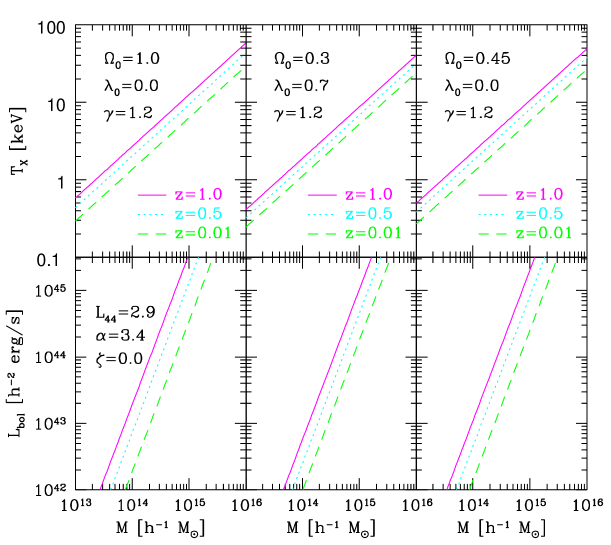
Figure 1: The X-ray temperature and luminosity as a function of cluster mass for three representative sets of cosmological parameters; $(\Omega_{0},\lambda_{0})=(1.0,0.0)$, $(0.3,0.7)$, and $(0.45,0.0)$ from left to right panels. The X-ray temperature (Upper panels) and the bolometric X-ray luminosity (Lower panels) are plotted at $z=1.0$ (solid lines), $0.5$ (dotted lines) and $0.01$ (dashed lines). We adopt the ratio of gas to virial temperature $\gamma=1.2$ (eq.[12]), and the non-evolving ($\zeta=0$) luminosity–temperature relation (eq.[13]) with the amplitude $L_{44}=2.9$ and the power-law index $\alpha=3.4$.

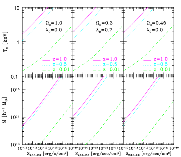
Figure 2: The X-ray temperature and cluster mass as a function of X-ray flux in the $0.5-2$ keV band. Different lines indicate results at different redshifts; $z=1.0$ (solid), $0.5$ (dotted) and $0.01$ (dashed).

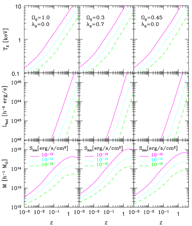
Figure 3: Temperature, bolometric luminosity and mass of clusters corresponding to the X-ray flux-limit $S_{\rm lim}$ as a function of redshift $z$; $S_{\rm lim}=10^{-13}$ (solid lines), $10^{-14}$ (dotted) and $10^{-15}$erg/s/cm² (dashed).

The relations among mass, temperature, luminosity and flux of X-ray clusters which we describe in the above do not depend on the power spectrum. For definiteness, however, we choose the same cosmological parameters as the above three models, and plot the results. Figure 1 shows the temperature $T_{\rm X}$ and the bolometric luminosity $L_{\rm bol}$, as a function of cluster mass $M$ at $z=0.01$ (dashed lines), 0.5 (dotted lines) and 1.0 (solid lines). Figure 2 plots $T_{\rm X}$ and $M$ as a function of X-ray flux $S_{0.5-2.0}$ for clusters at $z=0.01$ (dashed lines), 0.5 (dotted lines) and 1.0 (solid lines). Figure 3 shows $T_{\rm X}$, $L_{\rm bol}$ and $M$ of clusters at $z$ with the observed X-ray flux $S_{0.5-2.0}=10^{-13}$, $10^{-14}$ and $10^{-15}$erg/s/cm² in solid, dotted and dashed curves, respectively.

2.3 Evolution of luminosity–dependent bias

In order to complete a model for $\xi^{\rm S}_{\rm cl}(R,z;>S_{\rm lim})$, the two-point correlation function of X-ray clusters on a constant-time hypersurface at $z$, one has to specify a model for bias. Here we adopt a fitting formula for bias of Jing (1998), which improves an original proposal by Mo & White (1996) on the basis of high-resolution N-body simulations:

$$b(z,M)=\left[{0.5\delta_{c}^{4}\over\Delta^{4}(M,z)}+1\right]^{0.06-0.02n_{\rm eff}}\left[1-{1\over\delta_{c}}+{\delta_{c}\over\Delta^{2}(M,z)}\right].$$ (22)

In the above, $\Delta(M,z)$ is the density fluctuation smoothed over a (top-hat) mass scale of $M$ at the redshift $z$, $n_{eff}$ is the effective slope of the linear density power spectrum at the mass scale $M$ (see Jing 1998), $\delta_{c}=1.69$ is the critical density contrast for the spherical collapse. To be specific, Jing (1998) carried out several simulations in four scale-free models and three representative CDM models employing $256^{3}$ particles. Each model is simulated with three or four different realizations. The dark matter halos are identified using the friends-of-friends algorithm using the linking length of 0.2 times the mean particle separation. Thus the above formula (22) applies for the virialized dark halo defined according to the Press – Schechter theory, and is appropriate for the clusters of galaxies.

Combining the results in the previous subsection, we translate the above bias factor into a function of X-ray flux limit according to

$$b_{\rm eff}(z,>S_{\rm lim}) = {\displaystyle\int_{M_{\rm lim}(S_{\rm lim})}^{\infty}dM~{}b(z,M)~{}n_{\scriptscriptstyle{\rm PS}}(z,M)\over\displaystyle\int_{M_{\rm lim}}^{\infty}dM~{}n_{\scriptscriptstyle{\rm PS}}(z,M)}$$ (23)

$$n_{\scriptscriptstyle{\rm PS}}(z,M) = -\left({2\over\pi}\right)^{1/2}{3\Omega_{0}H_{0}^{2}\over 8\pi GM}{\delta_{c}\over\Delta^{2}(M,z)}{d\Delta(M,z)\over dM}\exp\left[-{\delta_{c}^{2}\over 2\Delta^{2}(M,z)}\right],$$ (24)

where $n_{\scriptscriptstyle{\rm PS}}(z,M)$ is the Press – Schechter mass function. Given the flux limit $S_{\rm lim}$, the corresponding luminosity $L_{\rm lim}(z)$ for a cluster located at $z$ is computed from equation (15) with the luminosity distance $d_{\rm L}(z)$. Then we solve equations (13) and (14) for $T_{\rm lim}(z)=T_{{\rm\scriptscriptstyle gas}}$, and finally obtain $M_{\rm lim}(z)$ using equation (12).

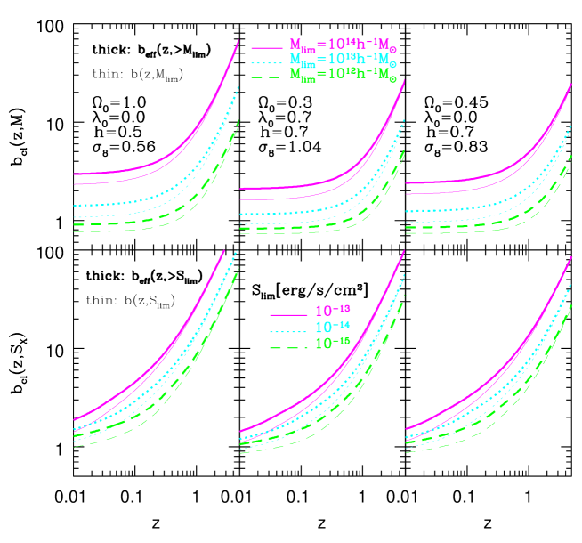
Figure 4: Evolution of bias for clusters selected by mass and X-ray flux in SCDM, LCDM and OCDM models; Upper panels: bias for different mass limits, $M_{\rm lim}=10^{14}h^{-1}M_{\odot}$, $10^{13}h^{-1}M_{\odot}$ and $10^{12}h^{-1}M_{\odot}$ in solid, dotted and dashed lines, respectively. Thin lines indicate the result for $b(z,M_{\rm lim})$ while thick lines for the effective bias $b_{\rm eff}(z,>M_{\rm lim})$. Lower panels: bias for different flux limits, $S_{\rm lim}=10^{-13}$, $10^{-14}$ and $10^{-15}$erg/s/cm² in solid, dotted and dashed lines, respectively. Thin lines indicate the result for $b(z,S_{\rm lim})$ while thick lines for the effective bias $b_{\rm eff}(z,>S_{\rm lim})$.

Figure 4 plots the evolution of $b_{\rm eff}(z,>M)$, $b(z,M)$, $b_{\rm eff}(z,>S_{\rm lim})$ and $b(z,S_{\rm lim})$ for our model of X-ray clusters. As noted in Figure 3 of Jing (1998), the fitting formula is accurate within 10 percent for $M\lower 2.15277pt\hbox{$\;\buildrel<\over{\sim}\;$}10^{14}h^{-1}M_{\odot}$ on linear scales. We checked the accuracy of the fit using the more recent numerical simulations, and made sure that the fit is accurate better than 20 percent even at $M=10^{15}h^{-1}M_{\odot}$. In any case, the fraction of such massive clusters is significantly smaller according to equation (24), and the difference of the fit and simulations to that level hardly changes our results in reality. We should note here, however, that the bias factor becomes scale-dependent for scales below $\sim 5{\hbox{$h^{-1}$}{\rm Mpc}}$, and then our assumption of linear and scale-independent bias breaks down. Thus while our predictions on linear scales $\lower 2.15277pt\hbox{$\;\buildrel>\over{\sim}\;$}5{\hbox{$h^{-1}$}{\rm Mpc}}$, which we are mostly interested in, are reliable, those on smaller scales should be interpreted simply to show the various effects qualitatively.

2.4 The light-cone effect

The two-point correlation function on the light-cone is properly formulated by Yamamoto & Suto (1999). In the present context, their formula yields the following expression for the two-point correlation functions of clusters brighter than the X-ray flux-limit $S_{\rm lim}$:

$$\xi^{\rm LC}_{\rm X-cl}(R;>S_{\rm lim})={{\displaystyle\int_{z_{\rm max}}^{z_{\rm min}}dz{dV_{\rm c}\over dz}~{}n_{0}^{2}(z)\xi^{\rm S}_{\rm cl}(R,z(r);>S_{\rm lim})}\over{\displaystyle\int_{z_{\rm max}}^{z_{\rm min}}dz{dV_{\rm c}\over dz}~{}n_{0}^{2}(z)}}$$ (25)

where $R$ is the comoving separation of a pair of clusters, $z_{\rm max}$ and $z_{\rm min}$ denote the redshift range of the survey, and $\xi^{\rm S}_{\rm cl}(R,z;>S_{\rm lim})$ is the corresponding two-point correlation function on a constant-time hypersurface at $z$ in redshift space (eq.[8]). The comoving number density of clusters in the flux-limited survey, $n_{0}(z;>S_{\rm lim})$, is computed by integrating the Press – Schechter mass function as

$$n_{0}(z;>S_{\rm lim})=\int_{M_{\rm lim}(S_{\rm lim})}^{\infty}n_{{\scriptscriptstyle{\rm PS}}}(M,z)dM.$$ (26)

Finally the comoving volume element per unit solid angle is

$${dV_{\rm c}\over dz}={d_{\scriptscriptstyle C}^{2}(z)\over H(z)}.$$ (27)

While equation (25) was originally derived for the cosmological models with flat spatial geometry (Yamamoto & Suto 1999), we assume that the formula is valid for the cosmological models with open geometry. Note also that this expression for the light-cone effect looks rather different from that adopted by Mataresse et al. (1997) and Moscardini et al. (1999a), but that both lead to fairly similar results quantitatively; see Yamamoto & Suto (1999) for detailed comparison and discussion.

The formula (25) is useful in making theoretical predictions, but $n_{0}(z)$ itself is not directly observable (unless the cosmological parameters are specified). Instead it can be rewritten in terms of the redshift distribution of clusters per unit solid angle with an X-ray flux $S>S_{\rm lim}$:

$$\xi^{\rm LC}_{\rm X-cl}(R;>S_{\rm lim})={{\displaystyle\int_{z_{\rm min}}^{z_{\rm max}}{H(z)dz\over d_{\scriptscriptstyle C}^{2}(z)}\left({dN\over dz}\right)^{2}\xi^{\rm S}_{\rm cl}(R,z;>S_{\rm lim})}\over{\displaystyle\int_{z_{\rm min}}^{z_{\rm max}}{H(z)dz\over d_{\scriptscriptstyle C}^{2}(z)}\left({dN\over dz}\right)^{2}}},$$ (28)

and $dN/dz$ which is related to $n_{0}(z)$ as

$${dN\over dz}(z,>S_{\rm lim}) = n_{0}(z;>S_{\rm lim})~{}{dV_{\rm c}\over dz}.$$ (29)

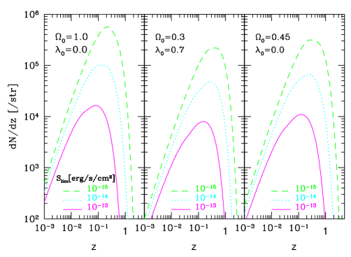
Figure 5: Redshift distribution functions for X-ray flux-limited clusters; $S_{\rm lim}=10^{-13}$, $10^{-14}$ and $10^{-15}$erg/s/cm² in solid, dotted and dashed lines, respectively.

Figure 5 plots the redshift distribution function for X-ray flux-limited clusters with $S_{\rm lim}=10^{-13}$, $10^{-14}$ and $10^{-15}$ erg/s/cm². It is interesting to note that $M_{\rm lim}(z)$ corresponding to a fixed $S_{\rm lim}$ decreases for $z\lower 2.15277pt\hbox{$\;\buildrel>\over{\sim}\;$}1$. In fact this behavior is understood from equations (12) to (15); $M_{\rm lim}(z)\propto T_{\rm lim}^{3/2}(z)/(1+z)^{3/2}\propto L_{\rm lim}^{3/2\alpha}(z)/(1+z)^{3/2}\propto d_{\scriptscriptstyle L}^{3/\alpha}(z)/(1+z)^{3/2}$.

3 Predictions for correlations in X-ray flux-limited surveys of clusters of galaxies

3.1 Nonlinear evolution, redshift-space distortion and light-cone effect

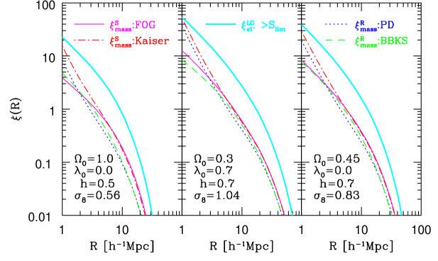
Figure 6: Light-cone and redshift-space distortion effects on two-point correlation functions of clusters; real-space mass correlation functions at $z=0$ in linear theory using the BBKS transfer function (dashed lines) and in a nonlinear model by PD (dashed lines). Redshift-space mass correlation functions at $z=0$ with the Kaiser distortion (dot-dashed lines) and with the Kaiser distortion and finger-of-god (thin solid lines). Thick solid lines indicate our predictions for the cluster correlation functions on the light cone in redshift space (the X-ray flux limit $S_{\rm lim}=10^{-14}$erg/s/cm²).

While our predictions based on the modeling described in the previous section include various important effects, it would be instructive to discuss them separately first. For that purpose, we plot in Figure 6 several different predictions for two-point correlation functions in which some of the effects are artificially turned off; linear and nonlinear mass correlations in real space at $z=0$ using the Bardeen et al. (1986; BBKS) and PD formulae for mass power spectra, cluster correlations with linear redshift-space distortion (Kaiser 1987) and with full redshift-space distortion, at $z=0$ using the fitting formula of Mo, Jing & Börner (1997) to compute $\sigma_{v}$. These should be compared with our final predictions on the light-cone in redshift space (eq.[8]).

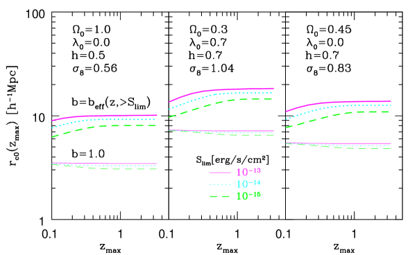
Figure 9: Correlation lengths of clusters in SCDM (Left panels), LCDM (Middle panels), and OCDM (Right panels) as a function of the survey depth, $z_{\rm max}$. The X-ray flux-limit $S_{\rm lim}$ is $10^{-13}$ (solid), $10^{-14}$ (dotted) and $10^{-15}$erg/s/cm² (dashed lines). Thin lines indicate the predictions in the $b(z)=1$ model for comparison.

The qualitative features illustrated in Figure 6 can be understood as the combination of the following effects; the nonlinear gravitational evolution increases the correlation on small scales, while redshift-space distortion decreases (enhances) the amplitudes on small (large) scales. The correlation length defined by eq.[30] below, for inscance, is enhanced in redshift space by 50 percent for SCDM and 20 percent for LCDM and OCDM in comparison with those in real space. The light-cone effect averages the amplitude over a range of redshift which is generally expected to decrease the correlation if the clustering amplitude at higher $z$ decreases according to linear theory. In reality, however, $b_{\rm eff}(z)$ increases more rapidly than the linear growth rate $D_{1}(z)$ at higher $z$, and therefore the clustering amplitude evaluated on the light cone for a given $S_{\rm lim}$ increases as $z$ (see Fig.9 below).

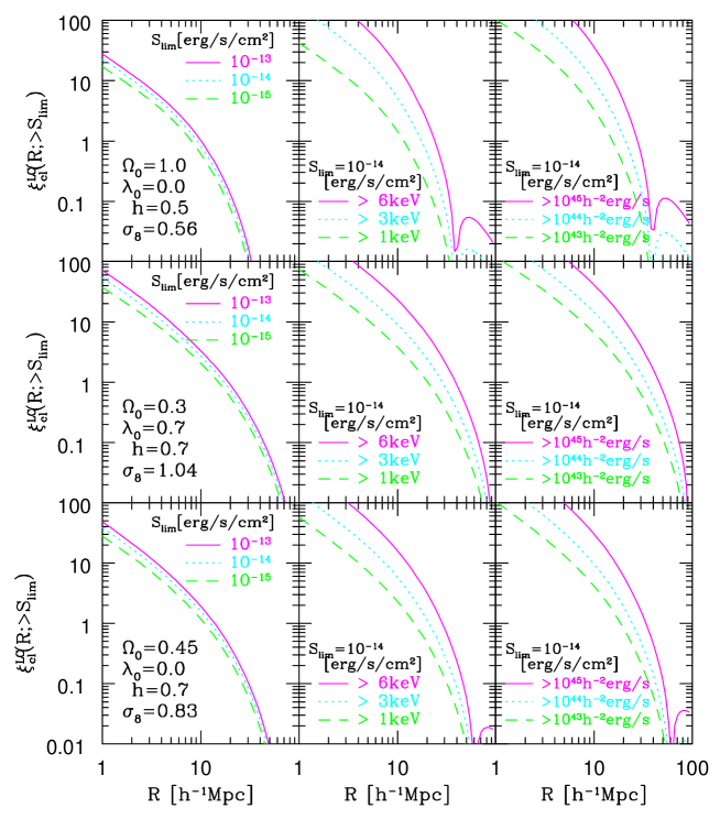
Figure 7: Two-point correlation functions of clusters in SCDM (Top panels), LCDM (Middle panels), and OCDM (Bottom panels) for different selection criteria. Left panels: the X-ray flux limit $S_{\rm lim}=10^{-13}$ (solid lines), $10^{-14}$ (dotted) and $10^{-15}$erg/s/cm² (dashed). Central panels: clusters with the temperature larger than $1$ (solid), $3$ (dotted) and $6$keV (dashed) in the X-ray flux-limited sample ($S_{\rm lim}=10^{-14}$erg/s/cm²). Right panels: clusters with the bolometric luminosity larger than $10^{45}$ (solid), $10^{44}$ (dotted) and $10^{43}h^{-2}$erg/s/cm² (dashed) in the X-ray flux-limited sample ($S_{\rm lim}=10^{-14}$erg/s/cm²).

Nevertheless this is not what we observe in a flux-limited survey. If the survey flux-limit $S_{\rm lim}$ becomes smaller, the sample includes both less luminous clusters at low $z$ and more luminous clusters at high $z$. While the latter shows stronger bias, the former should exhibit weaker bias. Thus averaging over the light-cone volume, their effect on the overall clustering amplitude is fairly compensated. This explains why the overall results are not so sensitive to $S_{\rm lim}$ as shown in left panels of Figure 7.

3.2 Effect of the selection function

If the temperature of an individual cluster in an X-ray flux-limited sample is determined observationally, one can construct a temperature-limited subsample. Similarly one can construct a luminosity-limited subsample from the flux-limited sample with the redshift information of each cluster. If the underlying luminosity–temperature relation (eq. [13]) had no dispersion, these two subsamples would be essentially the same. In reality, however, the finite amount of the dispersions would lead to different predictions for those subsamples, which will provide further and independent information on the cluster models. This is particularly the case here since the bias is highly sensitive to the mass, and therefore to the temperature and luminosity, of a cluster.

Figure 7 shows our predictions for $\xi^{\rm LC}_{\ cl}(R)$ for cluster samples selected with different flux-limit $S_{\rm lim}$ (left panels), and with temperature and absolute bolometric luminosity limits, $T_{\rm lim}$ and $L_{\rm lim}$ (middle and right panels). For the latter two cases, $S_{\rm lim}=10^{-14}$erg/s/cm² is assumed for definiteness. As explained in the previous subsection, the results are insensitive to $S_{\rm lim}$, but very sensitive to $T_{\rm lim}$ and $L_{\rm lim}$, reflecting the strong dependence of the bias on the latter quantities.

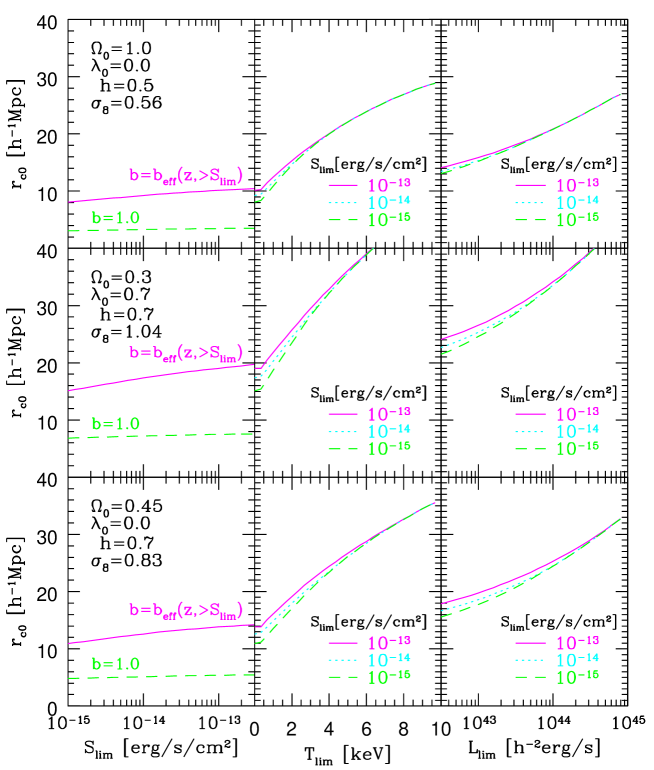
Figure 8: Correlation lengths of clusters $r_{\rm c0}$ in SCDM (Top panels), LCDM (Middle panels), and OCDM (Bottom panels) for different selection criteria. Left panels: $r_{\rm c0}$ for the X-ray flux-limited clusters. Dashed lines refer to the results in which the bias parameter is set to unity, while solid lines indicate our predictions. Central panels: $r_{\rm c0}$ as a function of the temperature limit for the X-ray flux-limited sample of $S_{\rm lim}=10^{-13}$ (solid lines), $10^{-14}$ (dotted) and $10^{-15}$erg/s/cm² (dashed). Right panels: $r_{\rm c0}$ as a function of the bolometric luminosity limit for the X-ray flux-limited sample of $S_{\rm lim}=10^{-13}$ (solid lines), $10^{-14}$ (dotted) and $10^{-15}$erg/s/cm² (dashed).

To see this in a somewhat different manner, we plot in Figure 8 the correlation length $r_{c0}(S_{\rm lim})$ defined through

$$\xi^{\rm LC}_{\rm cl}(r_{c0};>S_{\rm lim})=1,$$ (30)

as a function of $S_{\rm lim}$, $T_{\rm lim}$ and $L_{\rm lim}$. For the latter two cases, $S_{\rm lim}=10^{-14}$erg/s/cm² is assumed as in Figure 7. Again it is clear that the results are fairly insensitive to $S_{\rm lim}$, but are sensitive to the bias factor, which results in the strong dependence of $r_{c0}$ on $T_{\rm lim}$ and $L_{\rm lim}$.

The value of $r_{c0}(S_{\rm lim})$ also depends on the depth of the survey via the light-cone effect and the evolution of bias and mass fluctuations (Fig.9). As a result of the several competing effects, $r_{c0}(S_{\rm lim})$ increases, albeit very weakly, as $z_{\rm max}$ becomes larger.

3.3 Dependence on $\Omega_{0}$

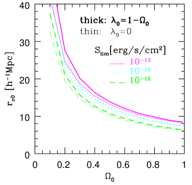
Figure 10: Correlation lengths of clusters as a function of $\Omega_{0}$. The shape parameter of the spectrum $\Gamma$ is fixed as $\Omega_{0}h\exp[-\Omega_{\rm b}(1+\sqrt{2h}\Omega_{0}^{-1})]$ with $\Omega_{\rm b}h^{2}=0.015$ and $h=0.7$. The X-ray flux-limit $S_{\rm lim}$ is $10^{-13}$ (solid lines), $10^{-14}$ (dotted) and $10^{-15}$erg/s/cm² (dashed). For each $S_{\rm lim}$, we plot the case of $\lambda_{0}=1-\Omega_{0}$ in thick lines, and $\lambda_{0}=0$ in thin lines.

For a cosmological application of the present result, it is interesting to examine how the $r_{c,0}(S_{\rm lim})$ depends on $\Omega_{0}$. This is summarized in Figure 10, where we fix the value of the fluctuation amplitude $\sigma_{8}$ adopting the cluster abundance constraint (eq.[11]), and consider both $\lambda_{0}=1-\Omega_{0}$ (thick lines) and $\lambda_{0}=0$ (thin lines). We set the shape parameter of the spectrum $\Gamma$ as $\Omega_{0}h\exp[-\Omega_{\rm b}(1+\sqrt{2h}\Omega_{0}^{-1})]$ with $\Omega_{\rm b}h^{2}=0.015$ and $h=0.7$. If we adopt such spectra, the correlation length in $\lambda_{0}=1-\Omega_{0}$ model is generally larger than that in $\lambda_{0}=0$ model, largely reflecting the dependence of $\sigma_{8}$ on $\lambda_{0}$ (eq.[11]). Again the results are not sensitive to the flux limit $S_{\rm lim}$. The dependence on $\Omega_{0}$ is rather strong, and these predictions combined with the future observational results will be able to break the degeneracy of the cosmological parameters.

4 Conclusions and discussion

We have presented a detailed methodology to predict the two-point correlation functions for X-ray flux-limited samples of clusters of galaxies, fully taking into account the redshift-space distortion, nonlinear gravitational evolution of mass fluctuations, evolution of bias, the light-cone effect and the observational selection function. While our method is similar to the recent model of Moscardini et al. (1999a) in many respects, the most important difference is that we incorporated both linear and nonlinear redshift-space distortion following the prescription of Suto et al. (1999), Yamamoto, Nishioka & Suto (1999) and Magira, Jing & Suto (2000).

The predictions for correlations of clusters are most sensitive to the model of bias among others. Fortunately, the Press – Schechter theory provides a quite reliable bias model for clusters (Mo & White 1996; Jing 1998), which is in marked contrast with a model for galaxy and quasar bias. Thus one can make quantitative and detailed model predictions once a set of the cosmological parameters are specified. These predictions can be checked against the flux-limited samples of clusters from the future X-ray satellites including Astro-E, Chandra, and XMM. It is particularly interesting to probe the value of $\Omega_{0}$ and the degree of non-Gaussianity by combining this comparison and the cluster abundance (Kitayama, Sasaki, & Suto 1998; Koyama, Soda, & Taruya 1999).

We should note, however, that the current methodology is reliable only for linear scales; on small scales ($\lower 2.15277pt\hbox{$\;\buildrel<\over{\sim}\;$}5{\hbox{$h^{-1}$}{\rm Mpc}}$), the approximation of the linear and scale-independent bias breaks down. In addition, the projection effect becomes inevitably important below a few $h^{-1}$Mpc scales even for the X-ray selected samples, and the observational data analysis itself becomes non-trivial.

While the selection function for the future survey would not exactly match those in our examples, it is straightforward to make suitable predictions on the basis of the present formalism at least on linear scales, and we hope that we have already presented all the basic and qualitative features of the clustering statistics.

After submitting this paper, Moscardini et al. (1999b) posted a quite similar paper on the clustering of X-ray selected galaxy clusters. They predicted the correlation lengths at $S_{\rm lim}=10^{-14}$erg/s/cm² of 7 and 12 $h^{-1}$Mpc in SCDM and LCDM models, respectively (their Fig.7), which should be compared with our predictions of 9 and 17 $h^{-1}$Mpc (Fig.8). While our models adopt slightly different values for the shape parameter $\Gamma$, and the normalization of fluctuations, $\sigma_{8}$, it is clear that our correlation lengths are systematically larger by $30\sim 40$ percent level. This should be ascribed to be the redshift-distortion effect which they neglect in their analysis. In fact, this difference is comparable to the cosmological model dependence which they showed in their Figure 7, clearly suggesting the importance of the effect to this level. Apart from this difference, however, our results are consistent with each other.

We thank an anonymous referee for detailed comments which improved the presentation of the earlier manuscript. Y.P.J. and T.K. gratefully acknowledge the fellowship from the Japan Society for the Promotion of Science. Part of numerical computations was carried out on VPP300/16R and VX/4R at ADAC (the Astronomical Data Analysis Center) of the National Astronomical Observatory, Japan, as well as at RESCEU (Research Center for the Early Universe, University of Tokyo) and KEK (High Energy Accelerator Research Organization, Japan). This research was supported in part by the Grants-in-Aid by the Ministry of Education, Science, Sports and Culture of Japan to RESCEU (07CE2002) and to K.Y. (11640280), and by the Inamori Foundation.

REFERENCES

Bahcall, N.A. & Soneira, R.M. 1983, ApJ, 270, 20

Bahcall, N.A. 1988, ARA&A, 26, 631

Bahcall, N.A. & Cen, R.Y. 1993, ApJ, 407, L49

Barbosa, D., Bartlett, J. G., Blanchard, A., & Oukbir, J. 1996, AA, 314, 13

Bardeen, J. M., Bond, J. R., Kaiser, N., & Szalay, A. S. 1985 , ApJ, 304, 15 (BBKS)

Borgani, S., Plionis, M., & Kolokotronis, V. 1999, MNRAS, 305, 866

Burns, J.F. et al. 1996, ApJ, 467, 49

Cole, S., Fisher, K. B., & Weinberg, D. H. 1994, MNRAS, 267, 785

Cole, S., Fisher, K. B., & Weinberg, D. H. 1995, MNRAS, 275, 515

David, L. P., Slyz, A., Jones, C., Forman, W., & Vrtilek, S. D. 1993, ApJ, 412, 479

Ebeling, H., Edge, A. C., Fabian, A.C., Allen, S. W., & Crawford C. S. 1997, ApJ, 479, L101

Ebeling, H., Voges, W., Böhringer, H., Edge, A. C., Huchra, J. P., & Briel, U. G. 1996, MNRAS, 281, 799

Eke, V. R., Cole, S., & Frenk, C. S. 1996, MNRAS, 282, 263

Hamilton, A. J. S. 1998, in “ The Evolving Universe. Selected Topics on Large-Scale Structure and on the Properties of Galaxies”, (Kluwer: Dordrecht), p.185.

Jing, Y. P. 1998, ApJ, 503, L9

Jing, Y.P., Fang, L. Z. 1994, ApJ, 432, 438

Jing, Y.P., Mo H.J., Börner, G., Fang, L.Z. 1993, ApJ, 411, 450

Kaiser, N. 1984, ApJ, 284, L9

Kaiser, N. 1987, MNRAS, 227, 1

Kitayama, T., Sasaki,S., & Suto, Y. 1998, PASJ, 50, 1

Kitayama, T., & Suto, Y. 1996, ApJ, 469, 480

Kitayama, T., & Suto, Y. 1997, ApJ, 490, 557

Klypin, A.A. & Kopylov, A.I., 1983, Sov.Astron.Lett., 9, 75

Koyama, K., Soda, J., & Taruya, A. 1999, MNRAS, in press (astro-ph/9903027).

Magira, H., Jing, Y. P., & Suto, Y. 2000, ApJ, 528, January 1st issue, in press (astro-ph/9907438)

Makino, N., Sasaki, S., & Suto, Y. 1998, ApJ, 497, 555

Masai, K. 1984, Ap&SS, 98, 367

Matarrese, S., Coles, P., Lucchin, F., & Moscardini, L. 1997, MNRAS, 286, 115

Matsubara, T., & Suto, Y. 1996, ApJ, 470, L1

Matsubara, T., Suto, Y., & Szapudi, I. 1997, ApJ, 491, L1

Mo, H. J., Jing, Y. P., & Börner, G. 1997, MNRAS, 286, 979

Mo, H. J., & White, S. D. M. 1996, MNRAS, 282, 347

Moscardini, L., Coles, P., Lucchin, F., & Matarrese, S. 1998 , MNRAS, 299, 95

Moscardini, L., Matarrese, S., De Grandi, S. & Lucchin, F. 1999a, MNRAS, submitted (astro-ph/9904282).

Moscardini, L., Matarrese, S., Lucchin, F., & Rosati, P. 1999b, MNRAS, submitted (astro-ph/9909273).

Mushotzky, R. F., & Scharf, C. A. 1997, ApJ;482;L13.

Nakamura, T. T., Matsubara, T., & Suto, Y. 1998, ApJ, 494, 13

Nishioka, H., & Yamamoto, K. 1999, ApJ, 520, 426

Peacock, J. A., & Dodds, S. J. 1996, MNRAS, 280, L19 (PD)

Ponman, T. J., Bourner, P. D. J., Ebeling, H., & Böhringer, H. 1996, MNRAS, 283, 690

Rosati, P., Della Ceca, R., Norman, C., & Giacconi, R. 1998, ApJ, 492, L21

Suto, Y., Magira, H., Jing, Y. P., Matsubara, T., & Yamamoto, K. 1999, Prog.Theor.Phys.Suppl., 133, 183

Suto, Y., Sasaki, S. & Makino, N. 1998, ApJ, 509, 544

Ueda, H., Itoh, M., & Suto, Y. 1993, ApJ, 408, 3

Viana, P. T. P., & Liddle, A. R. 1996, MNRAS, 281, 323

Watanabe, T., Matsubara, T., & Suto, Y. 1994, ApJ, 432, 17

White, S. D. M., Efstathiou, G., & Frenk, C. S. 1993, MNRAS, 262, 1023

Yamamoto, K., Nishioka, H., & Suto, Y. 1999, ApJ, 527, December 20 issue, in press (astro-ph/9908006)

Yamamoto, K., & Suto, Y. 1999, ApJ, 517, 1

Yoshikawa, K., Itoh, M., & Suto, Y. 1998, PASJ, 50, 203

Yoshikawa, K., Jing, Y.P., & Suto, Y. 1999, ApJ, submitted.

Yoshikawa, K., & Suto, Y. 1999, ApJ, 513, 549