The impact of viscosity on the morphology of gaseous flows in semidetached binary systems

Abstract—Results of 3D gas dynamical simulation of mass transfer in binaries are presented for systems with various values of viscosity. Analysis of obtained solutions shows that in the systems with low value of viscosity the flow structure is qualitatively similar to one for systems with high viscosity (see [1–6]). Presented calculations confirm that there is no shock interaction between the stream from $L_{1}$ and the forming accretion disk (‘hot spot’) at any value of viscosity.

INTRODUCTION

Earlier we have already considered the morphology of gaseous flows in semidetached binary systems [1–6]. Within the framework of the 3D numerical simulations we determined that the presence of rarefied circumbinary gas substantially changes the structure of gas flows in the system. In particular, the self-consistent solution does not include shock interaction between the stream of gas from the inner Lagrangian point $L_{1}$ and the forming accretion disk (‘hot spot’). However, these solutions were obtained for relatively high viscosity in the disk because the insufficient power of the computer used precluded fine grid calculations. In terms of the $\alpha$-disk the numerical viscosity was $\alpha\sim\hbox{$\,{}^{1}\!/_{2}$}$. At the same time, the problem of flow structure at low viscosity is of great interest. This is primarily because the modern simulations of dwarf novae are based on the assumption that the accretion disk has two states with low and high viscosity (see, e.g., [7–10]). The validity of this ‘limit cycle variation’ model has been confirmed by observational data (see, e.g., [10,11]).

The aim of this work is to investigate the general morphology of gas flows in semidetached binary systems with low viscosity. Particular attention will be paid to the problem whether the flow structure remains the same with a decrease in viscosity, and, in particular, whether the stream-disk interaction retains its shock-free pattern as was shown in [1,2] for relatively high viscosity. Study of stream-disk interaction and the related problem of the absence of ‘hot spot’ is of great importance for the interpretation of the observations.

In present work we used Euler equations describing the flow of unviscous gas (similar to works [1–6]). Nevertheless, the behavior of the solution is influenced by the numerical viscosity. The presence of the only numerical viscosity and the absence of the physical one in the simulation restricts detailed investigation of the problem, while the dependence of the solution on the viscosity can be described qualitatively. Because numerical viscosity (assuming the finite–difference scheme is already chosen) depends on the spatial and time resolution, the viscosity dependence of the solution can be obtained in sequential runs with decreasing size of the gridcell.

1 THE MODEL

Let us consider the semidetached binary system with mass ratio $q=1$. To describe the gas flow in this binary system we used the 3D system of Euler equations

$$\frac{\partial\rho}{\partial t}+\frac{\partial\rho u}{\partial x}+\frac{\partial\rho v}{\partial y}+\frac{\partial\rho w}{\partial z}=0\,,$$

$$\frac{\partial\rho u}{\partial t}+\frac{\partial(\rho u^{2}+P)}{\partial x}+\frac{\partial\rho uv}{\partial y}+\frac{\partial\rho uw}{\partial z}=-\rho\frac{\partial\Phi}{\partial x}+2\Omega v\rho\,,$$

$$\frac{\partial\rho v}{\partial t}+\frac{\partial\rho uv}{\partial x}+\frac{\partial(\rho v^{2}+P)}{\partial y}+\frac{\partial\rho vw}{\partial z}=-\rho\frac{\partial\Phi}{\partial y}-2\Omega u\rho\,,$$

$$\frac{\partial\rho w}{\partial t}+\frac{\partial\rho uw}{\partial x}+\frac{\partial\rho vw}{\partial y}+\frac{\partial(\rho w^{2}+P)}{\partial z}=-\rho{\displaystyle\partial\Phi\over\displaystyle\partial z}\,,$$

$$\frac{\partial\rho E}{\partial t}+\frac{\partial\rho uh}{\partial x}+\frac{\partial\rho vh}{\partial y}+\frac{\partial\rho wh}{\partial z}=-\rho u\frac{\partial\Phi}{\partial x}-\rho v\frac{\partial\Phi}{\partial y}-\rho w\frac{\partial\Phi}{\partial z}\,.$$

Here, $\rho$ denotes density; $u$, $v$, and $w$ are the $x$, $y$, and $z$ components of the velocity vector ${{\mathchoice{\hbox{$\displaystyle v$}}{\hbox{$\textstyle v$}}{\hbox{$\scriptstyle v$}}{\hbox{$\scriptscriptstyle v$}}}}=(u,v,w)$; $P$ is the pressure; $E=\varepsilon+\hbox{$\,{}^{1}\!/_{2}$}\cdot|{{\mathchoice{\hbox{$\displaystyle v$}}{\hbox{$\textstyle v$}}{\hbox{$\scriptstyle v$}}{\hbox{$\scriptscriptstyle v$}}}}|^{2}$ is the total specific energy; $h=\varepsilon+P/\rho+\hbox{$\,{}^{1}\!/_{2}$}\cdot|{{\mathchoice{\hbox{$\displaystyle v$}}{\hbox{$\textstyle v$}}{\hbox{$\scriptstyle v$}}{\hbox{$\scriptscriptstyle v$}}}}|^{2}$ is the total specific enthalpy; and $\Phi$ is the Roche potential:

$$\Phi({{\mathchoice{\hbox{$\displaystyle r$}}{\hbox{$\textstyle r$}}{\hbox{$\scriptstyle r$}}{\hbox{$\scriptscriptstyle r$}}}})=-\frac{GM_{1}}{|{{\mathchoice{\hbox{$\displaystyle r$}}{\hbox{$\textstyle r$}}{\hbox{$\scriptstyle r$}}{\hbox{$\scriptscriptstyle r$}}}}-{{\mathchoice{\hbox{$\displaystyle r$}}{\hbox{$\textstyle r$}}{\hbox{$\scriptstyle r$}}{\hbox{$\scriptscriptstyle r$}}}}_{1}|}-\frac{GM_{2}}{|{{\mathchoice{\hbox{$\displaystyle r$}}{\hbox{$\textstyle r$}}{\hbox{$\scriptstyle r$}}{\hbox{$\scriptscriptstyle r$}}}}-{{\mathchoice{\hbox{$\displaystyle r$}}{\hbox{$\textstyle r$}}{\hbox{$\scriptstyle r$}}{\hbox{$\scriptscriptstyle r$}}}}_{2}|}-\hbox{$\,{}^{1}\!/_{2}$}\Omega^{2}{\left({{\mathchoice{\hbox{$\displaystyle r$}}{\hbox{$\textstyle r$}}{\hbox{$\scriptstyle r$}}{\hbox{$\scriptscriptstyle r$}}}}-{{\mathchoice{\hbox{$\displaystyle r$}}{\hbox{$\textstyle r$}}{\hbox{$\scriptstyle r$}}{\hbox{$\scriptscriptstyle r$}}}}_{c}\right)}^{2}\,,$$

$\Omega=2\pi/P_{orb}$ is binary’s angular velocity; ${{\mathchoice{\hbox{$\displaystyle r$}}{\hbox{$\textstyle r$}}{\hbox{$\scriptstyle r$}}{\hbox{$\scriptscriptstyle r$}}}}_{1}$, ${{\mathchoice{\hbox{$\displaystyle r$}}{\hbox{$\textstyle r$}}{\hbox{$\scriptstyle r$}}{\hbox{$\scriptscriptstyle r$}}}}_{2}$ is the radius-vectors of centers of mass of system components; and ${{\mathchoice{\hbox{$\displaystyle r$}}{\hbox{$\textstyle r$}}{\hbox{$\scriptstyle r$}}{\hbox{$\scriptscriptstyle r$}}}}_{c}$ is the radius-vector of center of masses of a binary system. The calculations were carried out in the non-inertial Cartesian coordinate system rotating together with the binary system. Origin of coordinates is located in the center of a mass-losing component, ‘$x$’-axis is directed along the line connecting the centers of stars, from the mass-losing component to the accretor, ‘$z$’-axis is directed along the axis of rotation, and $y$’-axis is determined so that we obtain a right-hand coordinate system. To close the system of equations, we used the equation of state of ideal gas $P=(\gamma-1)\rho\varepsilon$, where $\gamma$ as it usually is the ratio of heat capacities. To mimic the system with radiating losses, we accept in the model the value of adiabatic index close to unit: $\gamma=1.01$, that corresponds to the case close to the isothermal one [12,13].

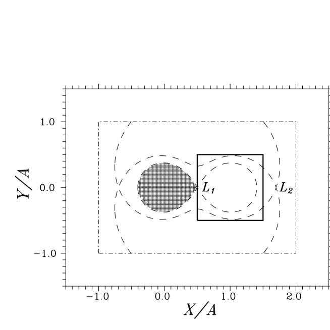
Figure 1: The calculation domains for the ‘complete’ (dash-dotted line) and ‘restricted’ (bold line) problems. Shaded region is the donor. The Roche equipotentials are shown by dashed lines.

Figure 2a: Isolines of density and velocity vectors in the equatorial plane for the run in the ‘complete’ region (see [6]). Filled circle is the accretor, dashed lines are the Roche equipotentials. The vector in the upper right corner corresponds to dimensionless velocity $v=3$. Bold line is the boundary (‘marginal’) flowline, along which the matter falls in the disk.

Figure 2b: Isolines of density and velocity vectors in the equatorial plane for the run in the ‘restricted’ calculation domain on the same grid as that shown on Fig. 2a. Filled circle is the accretor, dashed lines are the Roche equipotentials. The vector in the upper right corner corresponds to dimensionless velocity $v=3$. Bold line is the boundary (‘marginal’) flowline, along which the matter falls in the disk.

Figure 3: One-dimensional density profiles for ‘complete’ (dashed line) and ‘restricted’ runs (solid line). The density values are taken along the line in the equatorial plane passing near the $L_{1}$ point parallel to the ‘$y$’-axis ($x=\hbox{$\,{}^{1}\!/_{2}$}+h$, $z=0$).

Figure 4: Schematic presentation of gas dynamical flow patterns in semidetached binary systems. The Roche lobe (dashed lines), the accretor, the Lagrangian points, and the quasi-elliptic accretion disk are shown. Bold line is the shock wave formed as a result of interactions between the circumbinary envelope gas and the stream. The flowlines $a$, $b$, $c$, $d$ show the directions of gaseous flows in the system. Flowlines $a$, $b$, $d$ form the circumbinary envelope of the system, flowline $c$ is the gas flow leaving the system.

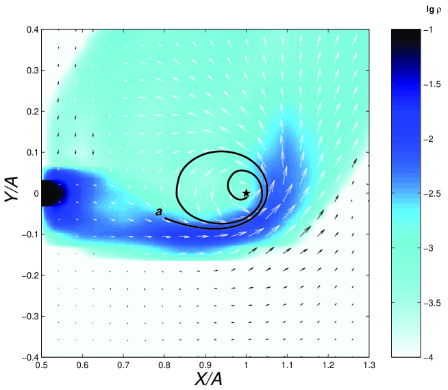
Figure 5a: The distribution of density over the equatorial plane for run ‘A’ (grid $31\times 31\times 17$). Arrows are the velocity vectors. Black asterisk is the accretor. Flowline $a$ bounding the accretion disk is also shown. Correspondence between density logarithm and gradation of grey color is shown on the scale.

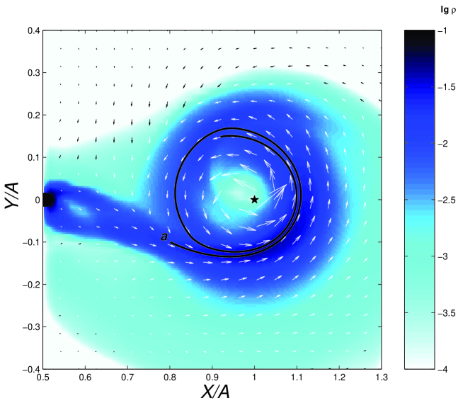
Figure 5b: The same as in Fig. 5a for run ‘B’ (grid $61\times 61\times 17$).

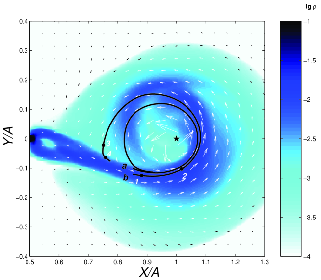
Figure 5c: The same as in Fig. 5a for run ‘C’ (grid $91\times 91\times 25$). In addition to flowline $a$ bounding the accretion disk, flowline $b$ passing through the shock is also shown. Zone ‘1-2’ of flowline $b$ corresponds to the place where gas stream from $L_{1}$ contacts with accretion disk, zone ‘3-4’ corresponds to the place of interaction between circumbinary gas and the stream (shock wave $I$).

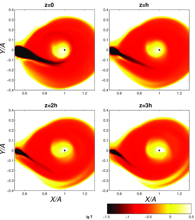
Figure 6: The distribution of dimensionless temperature over equatorial plane $z=0$ and the parallel planes $z=h$, $z=2h$, $z=3h$ for run ‘C’ (grid $91\times 91\times 25$). Here $h$ is the height of the gridcell that is approximately equal to $0.01A$. Black asterisk is the accretor.

Figure 7: Dimensionless temperature along flowline $b$, ref. Fig. 5c. Zone ‘1-2’ corresponds to the place of contact of the stream and the accretion disk, zone ‘3-4’ corresponds to the shock wave $I$.

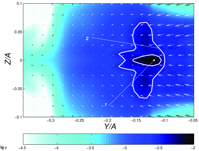
Figure 8: Distribution of density and velocity vectors in ‘$yz$’-plane passing through point $(\hbox{$\,{}^{9}\!/_{10}$},0,0)$, for run ‘C’ (grid $91\times 91\times 25$). Marker 1 designates the central part of the stream limited by isoline $\lg\rho=-2.3$. Marker 2 on isoline $\lg\rho=-2.5$ shows the front of shock wave $I$.

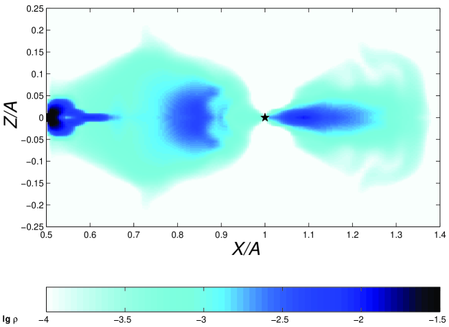
Figure 9: The distribution of density and velocities vectors in frontal plane (‘$xz$’-plane) for run ‘C’ (grid $91\times 91\times 25$). Black asterisk is the accretor.

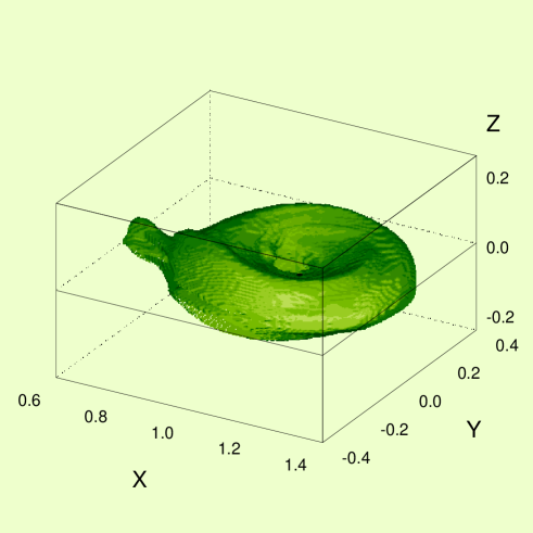
Figure 10a: 3D image of density iso-surface at level $\rho=10^{-3}$. Black circle is the accretor.

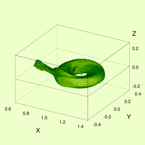
Figure 10b: The same as in Figure 10a for density $\rho=3\cdot 10^{-3}$.

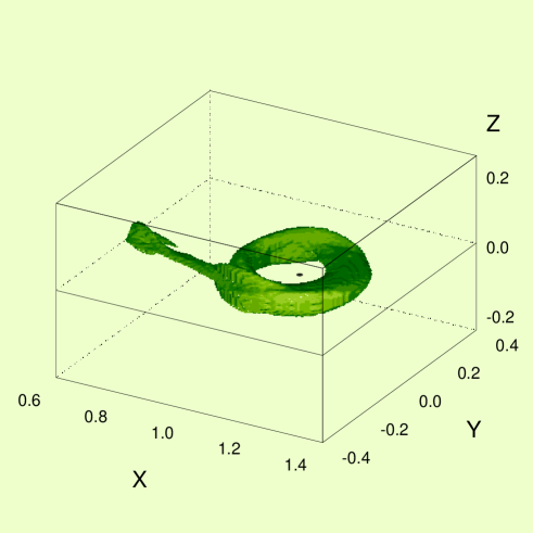
Figure 10c: The same as in Figure 10a for density $\rho=6\cdot 10^{-3}$.

To obtain numerical solution of the system of equations we used the Roe–Osher TVD scheme of a high approximation order [14,15] with Einfeldt modification [16]. The original system of equations was written in a dimensionless form. To do this, the spatial variables were normalized to the distance between the components $A$, the time variables were normalized to the reciprocal angular velocity of the system ${\Omega}^{-1}$, and the density was normalized to its value in the inner Lagrangian point $L_{1}$.

As it was noted above we decreased numerical viscosity by changing of the gridcell size. Unfortunately, the limited power of the computer used did not allow us to simulate the flow over a large domain (as in the calculations in [1–6] where the size of computational domain was 3 times larger than the binary system separation) on a fine grid. Therefore, similarly to works [17–20], the gas flow was simulated over a restricted domain that was set as parallelepipedon $[\hbox{$\,{}^{1}\!/_{2}$}A\ldots\hbox{$\,{}^{3}\!/_{2}$}A]\times[-\hbox{$\,{}^{1}\!/_{2}$}A\ldots\hbox{$\,{}^{1}\!/_{2}$}A]\times[0\ldots\hbox{$\,{}^{1}\!/_{4}$}A]$ (calculations were conducted only in the top half-space). A sphere with a radius of $\,{}^{1}\!/_{100}$ representing the accretor was cut out of the calculation domain. By way of illustration, the parameters of the calculation domain in the equatorial plane are shown in Fig. 1 (solid line); the dashed curves are the Roche equipotentials, and the dashed-dotted lines show the boundary of the calculation domain adopted in [1–6].

As the initial conditions we used rarefied gas with the following parameters $\rho_{0}=10^{-5}$, $p_{0}=10^{-4}/\gamma$, ${{\mathchoice{\hbox{$\displaystyle v$}}{\hbox{$\textstyle v$}}{\hbox{$\scriptstyle v$}}{\hbox{$\scriptscriptstyle v$}}}}_{0}=0$. The boundary conditions were determined as follows: we preset the conditions in a fictitious gridpoint corresponding to the inner Lagrangian point: $\rho(L_{1})=1$, $p(L_{1})=10^{-2}/\gamma$, $u(L_{1})=10^{-2}$, $v(L_{1})=w(L_{1})=0$; the velocity of sound in this gridpoint was equal to $c(L_{1})=10^{-1}$. In fictitious points located inside of the accretor and also in the fictitious points on the outer border except $L_{1}$ point all the parameters were taken equal to the initial (‘background’) values. The final (numerical) boundary conditions were determined by solving the Riemann problem between the gas parameters in fictitious gridpoints and the gas parameters in the closest gridpoint.

2 RESULTS

In [1–6] we studied the morphology of flow over a complete computational domain that is few times larger than binary separation $A$ and includes both system components (see Fig. 1). In these calculations the circumbinary envelope was found to play an important role in formation of the flow structure. The use of a restricted calculated domain in numerical model precludes the account of the circumbinary envelope and, hence, the ‘restricted’ solution can appreciably differ from the ‘complete’ one. Let us consider the effect of the restricted calculated domain on the solution. We compare the structure of flow from the ‘complete’ model [6] and the calculation obtained at the same grid in the restricted domain. Figures 2a and 2b depict isolines of density and the velocity vectors in the equatorial plane of the system for the ‘complete’ and the ‘restricted’ calculations, respectively. Figures 2a and 2b also represent the boundary (‘marginal’) flowline of the stream, along which the matter falls directly in the disk. Comparison of the results proves that the morphology of flows in the region near the disk in the ‘restricted’ problem reflects the basic features of flow patterns of the ‘complete’ solution. In particular, an accretion disk forming in the system has approximately the same linear size and shock waves $I$ and $II$ appear as a result of interaction of gas of the circumbinary envelope with the stream from $L_{1}$ (note that hereinafter the position of shock waves is determined by condensing of density isolines and the presence of mass flow through the surface). Meanwhile, in the ‘restricted’ problem the effect of the circumbinary envelope is taken into account not quite correctly. In particular, matter flows along the Roche lobe of a donor-star that result in the stripping of the atmosphere of a donor-star and essential increase in the rate of mass transfer in the system are not taken into account (see [2]). This fact causes essential change in the parameters of the stream of the ‘restricted’ problem in comparison to the ‘complete’ one (see Fig. 3 where one-dimensional distributions of density along a line parallel to ‘$y$’-axis and lying in equatorial plane are shown for ‘complete’ and the ‘restricted’ calculations). In particular, in the ‘restricted’ problem the stream flowing out from $L_{1}$ tends to extend to the characteristic value $\epsilon=c(L_{1})/A\Omega$ [21], and the density decreases along the cross-section of the stream by exponential law, while in the ‘complete’ problem the density of flowing matter is considerably determined by the stripping effect of the atmosphere of the donor-star. Moreover, the ‘restricted’ problem does not take account of the flow of the circumbinary gas returning in the system under the impact of Coriolis force (from the side of the stream which is opposite to the orbital motion). As a results, shock wave $III$ disappears in the ‘restricted’ problem but exists in the ‘complete’ one. Summarizing the results of comparison the ‘complete’ (the basic features of the obtained flow structure for ‘complete’ formulation are summarized on the schematic diagram – Fig. 4) and the ‘restricted’ problems, we can state that:

• In the ‘restricted’ problem the effect of the circumbinary envelope on the solution is considered not quite correctly. As a results, it causes, from one hand, qualitative changes of the solution: a part of flows of the circumbinary gas returning in the system is absent in the ‘restricted’ solution (flowlines $d$ and $b$ in Fig. 4), and, hence, shock wave $III$ disappears; on the other hand, quantitative changes: the parameters of stream change because the stripping effect is not taken into account, and, in particular, the thickness of the stream tends to decrease.

• The morphology of gaseous flows in the vicinity of the accretor in the ‘restricted’ and the ‘complete’ solutions is similar at a qualitative level. The partial account of the circumbinary envelope in the ‘restricted’ problem (e.g., the matter revolving around the accretor and interacting with a stream – see flowline $a$ in Fig. 4) allows one to obtain the solution similar to the ‘complete’ one. In particular, both in the ‘complete’ problem (see [1–6]) and in the ‘restricted’ solution the flow deflecting under the impact of gas of the circumbinary envelope approach to the disk at a tangent line and does not cause shock disturbances of the edge of disk (‘hot spot’). In both solutions the regions of superfluous energy release are located along the edge of stream facing towards the orbital motion where the interaction of the circumbinary envelope with the stream causes extended shock wave $I$ to form (see Figs 2,4).

The comparison of the ‘restricted’ and the ‘complete’ problems discussed above proves that stream–disk interaction can also be considered with some clauses in the ‘restricted’ problem. Therefore, we can conduct the fine grid calculations and, hence, to get the solutions at lower viscosity. Accordingly, we can study the impact of viscosity value on the flow structure in the vicinity of the accretor and consider the problem of ‘hot spot’ appearance at low viscosity.

To study the effect of viscosity we consider the results of three calculations with the various spatial resolution: $31\times 31\times 17$, $61\times 61\times 17$, and $91\times 91\times 25$ (hereinafter, ‘A’, ‘B’ and ‘C’ runs, respectively). In all the calculations the grid was taken uniform. In terms of $\alpha$-disk, the numerical viscosity of ‘A’, ‘B’ and ‘C’ runs corresponded to $\alpha\sim 0.08\div 0.1$, $0.04\div 0.06$, and $0.01\div 0.02$.

Comparison of the results of ‘A’, ‘B’ and ‘C’ runs among each other and with the results of study [20], where grid $200\times 200\times 50$ was used within the framework of the same problem setup allows one to study the impact of viscosity on the solution. Figures 5a, 5b and 5c show the fields of density and the velocity vectors in the equatorial plane of the system for ‘A’, ‘B’ and ‘C’ variants and also flowline $a$ bounding the accretion disk. Numerical analysis of the obtained solutions proves the shock-free interaction of the stream and the disk in all variants of calculations. The morphology of the stream-disk system is uniform and, hence, the ‘hot spot’ does not form. This fact is obvious from Fig. 6 showing the distributions of dimensionless temperature in ‘$xy$’-plane for run ‘C’ (at the minimal value of viscosity) for four values of ‘$z$’-coordinate: $z=0$ – the equatorial plane, $z=h$, $z=2h$, and $z=3h$, where the height of the gridcell $h\sim 0.01A$. The dimensionless temperature in point $L_{1}$ is equal to $10^{-2}$. To obtain the dimensional temperature one should multiply the dimensionless value by $GM/AR$, where $G$ is the gravitational constant, $M$ is the total mass of the system, $A$ is the system separation, $R$ is the gas constant. Analysis of the temperature fields shown in Fig. 6 proves the absence of the energy release zone in the place of contact of a stream and a disk, i.e. the absence of ‘hot spot’ at all values of ‘$z$’-coordinate. Consideration of the change in the gas parameters along the flowlines supports this conclusion. In particular, Fig. 7 depicts the change of dimensionless temperature along flowline $b$ (Fig. 5c), from which one may conclude that ‘hot spot’ is absent in the place of contact of a stream and a disk (zone ‘1-2’) and that the energy release region locates in the place of forming shock wave $I$ (zone ‘3-4’ in Figs. 5c and 7)

Comparative analysis of the obtained solutions proves (see, e.g., Fig. 5a,b,c) that increasing of spatial resolution and, hence, reduction of numerical viscosity causes reduction of diffusion spreading of the stream. In the runs with a thinner stream (‘B’ and ‘C’ runs, and the calculation in work [20]) gas of the circumbinary envelope tends to flow around the stream from above and from below. An illustration of this fact can be seen in Fig. 8 where the density field and the velocity vectors in ‘$yz$’-plane passing through point $(\hbox{$\,{}^{9}\!/_{10}$},0,0)$ are shown for ‘C’ run. The change of density (the increase in flow thickness) in the region where gas of the circumbinary envelope interacts with the stream is also obvious in Fig. 9 represented the density field in frontal plane (‘$xz$’-plane) for run ‘C’. The presence of the gas flowing around a stream may give the impression that shock interaction appears between the stream and the disk (see, for example, the three-dimensional image of iso-density surface in Fig. 10, and also the work [20]), though analysis of the solution unambiguously proves the smooth nature of this part of the flow.

In our studies [1–6] we structured the flow patterns as follows:

• disk is the matter of stream that immediately captured by the accretor and then is accreted;

• circumbinary envelope is all the rest matter. The part of this matter revolves around the accretor, interacts with the stream and then can be accreted.

Thus, we divided the matter of stream by a physical attribute: if gas leaves the system or then interacts with the initial stream, we consider this matter as not belonged to the disk. In the solutions with small viscosity there was additional part of the envelope: the matter that flows around a stream from above and from below. Analysis of the flowlines proves that this part of the envelope does not belong to the disk. The large part of this matter leaves the system or, rotating around the accretor gradually comes nearer to the equatorial plane and then it does collide with the flow. In addition to the definitions of works [1–6], it is worthwhile introducing an additional term: the ‘circumbinary halo’ describing the matter that: i) revolves around the accretor (it is gravitationally captured); ii) does not belong to the disk; iii) interacts with the stream (collides or flows around from above and from below); iv) then, after interaction, it can be either involved in accretion or leaves the system.

The change in numerical viscosity should inevitably result in the change of accretion rate. Analysis of ‘A’, ‘B’ and ‘C’ runs, as it can be expected, proves that in the calculations with smaller viscosity the rate of accretion decreases. Unfortunately, the detailed study of this question requires huge computing time that essentially exceeds the power of the computer used. The problem is that in the calculations with high viscosity that were presented in [1–6] the viscous time scale

$$\tau^{visc}=\frac{R_{disk}^{2}}{\nu}=\frac{R_{disk}^{2}}{\alpha c_{s}H}\,,$$

where $c_{s}$ is the velocity of sound, $H$ is the characteristic thickness of a disk, exceeded the gas dynamical time scale for the disk

$$\tau^{gas-dyn}=\frac{R_{disk}}{c_{s}}\,,$$

only slightly, that allowed one to reach the steady-state solution at the times of several orbital periods. At decreased viscosity the steady-state solution can hardly be obtained because restricted power of the computer used does not allow one to conduct the calculations for the periods of time larger than $\tau^{visc}$. Analysis of ‘C’ variant, i.e. the study of the mass of the disk and halo as functions of time, proves that the solution was not a steady-state even at the times larger than 15 orbital periods.

CONCLUSIONS

Obtained results of 3D numerical simulations of mass transfer in semidetached binaries demonstrate the absence of the ‘hot spot’ in self-consistent solution. This conclusion was made when considering systems with large value of viscosity (see [1–6]). Presented calculations confirm that there is no shock interaction between the stream from $L_{1}$ and the forming accretion disk (‘hot spot’) at any value of viscosity.

Analysis of obtained solutions shows that in the systems with various values of viscosity the stream from $L_{1}$ is deflected under the impact of gas of the circumbinary envelope and approaches to the disk at a tangent line, so does not cause shock disturbances of the edge of disk (‘hot spot’). The regions of superfluous energy release are located along the edge of stream facing towards the orbital motion. So we can conclude about the qualitative similarity of the flow structure for various values of viscosity. At the same time runs with low value of viscosity (when diffusion is weak and thickness of the stream is small) reveal an important role of the gas of the circumbinary envelope that flows around the stream from above and from below. We have introduced an additional term to describe this feature of the flow structure: the ‘circumbinary halo’.

REFERENCES

1. Bisikalo, D.V., Boyarchuk, A.A., Kuznetsov, O.A. & Chechetkin, V.M. 1997, Astron. Zh., 74, 880 (Astron. Reports, 41, 786; astro-ph/9802004)

2. Bisikalo, D.V., Boyarchuk, A.A., Kuznetsov, O.A. & Chechetkin, V.M. 1997, Astron. Zh., 74, 889 (Astron. Reports, 41, 794; astro-ph/9802039)

3. Bisikalo, D.V., Boyarchuk, A.A., Kuznetsov, O.A., Khruzina, T.S., Cherepashchuk, A.M. & Chechetkin, V.M. 1998, Astron. Zh., 75, 40 (Astron. Reports, 42, 33; astro-ph/9802134)

4. Bisikalo, D.V., Boyarchuk, A.A., Chechetkin, V.M., Kuznetsov, O.A. & Molteni, D. 1998, Monthly Notices Roy. Astron. Soc., 300, 39 (astro-ph/9805261)

5. Bisikalo, D.V., Boyarchuk, A.A., Kuznetsov, O.A. & Chechetkin, V.M. 1998, Astron. Zh., 75, 706 (Astron. Reports, 42, 621; astro-ph/9806013)

6. Bisikalo, D.V., Boyarchuk, A.A., Chechetkin, V.M., Kuznetsov, O.A. & Molteni, D. 1999, Astron. Zh. (in press; astro-ph/9907084)

7. Meyer, F. & Meyer-Hofmeister, E. 1981, Astron. Astrophys., 104, L10

8. Cannizzo, J.K., Chen, W. & Livio, M. 1995, Astrophys. J., 454, 880

9. Honma, F., Matsumoto, R. & Kato, S. 1993, Astrophys. J. Suppl., 210, 365

10. Szuszkievich, E. & Miller, J.C. 1997, Monthly Notices Roy. Astron. Soc., 287, 165

11. Cannizzo, J.K. 1993, Astrophys. J., 419, 318

12. Sawada, K., Matsuda, T. & Hachisu, I. 1986, Monthly Notices Roy. Astron. Soc., 219, 75

13. Bisikalo, D.V., Boyarchuk, A.A., Kuznetsov, O.A., Popov, Yu.P. & Chechetkin, V.M. 1995, Astron. Zh., 72, 367 (Astron. Reports, 39, 325)

14. Roe, P.L. 1986, Ann. Rev. Fluid Mech., 18, 337

15. Osher, S. & Chakravarthy, S. 1984, SIAM J. Numer. Anal., 21, 955

16. Einfeldt, B. 1988, SIAM J. Numer. Anal., 25, 294

17. Molteni, D., Belvedere, G. & Lanzafame, G. 1991, Monthly Notices Roy. Astron. Soc., 249, 748

18. Lanzafame, G., Belvedere, G. & Molteni, D. 1992, Monthly Notices Roy. Astron. Soc., 258, 152

19. Armitage, P.J. & Livio, M. 1996, Astrophys. J., 470, 1024

20. Makita, M., Miyawaki, K. & Matsuda, T. 1999, Monthly Notices Roy. Astron. Soc. (submitted; astro-ph/9809003)

21. Lubow, S.H. & Shu, F.H. 1975, Astrophys. J., 198, 383