The Lyman-alpha Forest and Heavy Element Systems of GB1759+7539111Based on observations obtained at the W. M. Keck Observatory, which is jointly operated by the University of California and the California Institute of Technology.
Abstract
We present observations of the high-redshift QSO GB1759+7539 () obtained with HIRES on the Keck 10m telescope. The spectrum has a resolution of FWHM = 7 km s-1, and a typical signal-to-noise ratio per 2 km s-1 pixel of 25 in the Ly forest region, and 60 longward of the Ly emission.
The observed Ly forest systems have a mean redshift of =2.7. The H I column density distribution is well described by a power law distribution with index in the range log. The Doppler width distribution is consistent with a Gaussian distribution of mean km s-1, and standard deviation km s-1 with a cut-off at km s-1. There is marginal evidence of clustering along the line of sight over the velocity range 100250 km s-1. The 1-point and 2-point joint probability distributions of the transmitted flux for the Ly forest were calculated, and shown to be very insensitive to the heavy element contamination. We could find no evidence of Voigt profile departures due to infalling gas, as observed in the simulated forest spectra.
Twelve heavy-element absorption systems were identified, including damped Lyman-alpha (DLA) systems at =2.62 and 2.91. The C, N, O, Al, Si, P, S, Mg, Fe, and Ni absorption features of these systems were studied, and the elemental abundances calculated for the weak unsaturated lines. The systems have metallicities of and . Both systems appear to have a low dust content. They show an over-abundance of -elements relative to Fe-peak elements, and an under-abundance of odd atomic number elements relative to even. Nitrogen was observed in both systems, and found to be under-abundant relative to oxygen, in line with the time delay model of primary nitrogen production. C II* was also seen, allowing us to determine an upper limit to the cosmic microwave background temperature at of T12.9K.
keywords:
cosmology: cosmic microwave background - galaxies: abundances - intergalactic medium - quasars: absorption lines - quasars: individual (GB1759+7539)1 Introduction
In recent years rapid progress has been made in observational and theoretical studies of Ly absorption lines in the spectra of high-redshift QSOs. Large telescopes have given us the opportunity of studying the lines in much greater detail than ever before, with large gains in both resolution and signal-to noise ratio (S/N) (e.g. Hu et al. 1995; Kirkman and Tytler 1997). At the same time, recent cosmological simulations, taking into account a photoionizing ultra-violet background, have suggested that the Ly clouds at high redshift develop naturally in a hierarchical structure-formation scenario (e.g. Cen et al. 1994; Miralda-Escudé et al. 1996). The detailed study of the Ly forest, and comparison with the results of such simulations is perhaps one of the best tests of cosmic structure-formation theories, providing a constraint in the era .
The heavy element systems observed in the line of sight to QSOs also provide a wealth of information about the formation of structure at high redshift. Understanding the chemical evolutionary history of galaxies is fundamental to the study of galaxy formation. The largest heavy element systems, damped Lyman-alpha systems (DLAs), are believed to be the progenitors of present day galaxies [Wolfe 1995]. They dominate the mass of neutral gas at redshift , a mass comparable with that of the stars in present day spiral disks, suggesting that DLAs are the source of most of material available for star formation at high redshift [Lanzetta et al. 1995]
Prochaska & Wolfe (1997) studied the kinematics of DLAs, concluding that there is evidence for rotation, supporting the theory that they are the progenitors of modern day disk galaxies. This result was disputed by Haehnelt, Steinmetz & Rauch (1997). CDM models infer that DLAs are more like the progenitors of dwarf galaxies, or galactic halos, a model that is backed by studies of heavy element abundances [Pettini et al. 1994, Lu et al. 1996a] which have found an abundance pattern more akin to halo stars than disk stars in our Galaxy.
Pettini et al. (1994) systematically studied the Zn, and Cr abundances in DLAs, and concluded that they had low metallicity, typically at , and that they have a much lower dust-to-gas ratio than the local interstellar medium. Although it is still unclear which population of galaxies gives rise to DLAs, it is apparent that the gas in DLAs is at an early stage in the chemical evolution of the object, and so abundance studies should give us an insight into the early stages of galaxy evolution.
In this paper, we present observations and analyses of the absorption spectrum of the QSO GB1759+7539 (). In §2 we describe the observations and data reduction methods. The analysis of the absorption lines, and identification of the heavy element lines is discussed in §3. Then, in §4, we present the main observational results concerning the Ly forest, including the column density, and Doppler width distributions, and the clustering properties, as indicated by the two point correlation function. The elemental abundances in the two damped systems are discussed in §5, where the dust content, and nucleosynthesis histories of the two objects are considered. §6 investigates the cosmic microwave background temperature at . The main conclusions are summarized in §7.
2 Observations and Data Reduction
The radio source, GB1759+7539 was selected from the Green Bank 5-GHz survey [Condon et al. 1989], and identified by Hook et al. (1996) as a high-redshift radio-loud QSO. Hook et al. noted that this object is optically very bright and hence it is ideal for high resolution spectroscopic study.
| Dates | Exposure time (s) | Wavelength range(Å) |
|---|---|---|
| 6 July 1997 | 9000 | 4115–6515 |
| 6 July 1997 | 6000 | 4140–6540 |
| 13 July 1997 | 6000 | 4115–6515 |
| 13 July 1997 | 9000 | 4140–6540 |
The data used in the present study were obtained in two nights (see Table 1) using the High Resolution Echelle Spectrometer (HIRES) on the 10m Keck telescope [Vogt 1992], with the TeK 2048x2048 CCD. The FWHM of the instrument profile was found to be about 7 km s-1. The HIRES setup is such that complete spectral coverage is only possible for Å, so we used two partially overlapping setups to obtain complete coverage over the wavelength range 4116 - 6540 Å. This leads to fairly large variations in the S/N from region to region in the final spectrum.
Each image was bias and flat-field corrected using IRAF routines. The cosmic rays were flagged using a median filter and given zero weight in the individual frames. The sky-subtracted optical spectra were then optimally extracted, along with a one-sigma error estimate, calibrated to vacuum heliocentric wavelengths, and flux calibrated.
Even after flux calibration, there were some inexplicable low-order variations in the flux level of some of the images. The variations were echelle order dependent, and therefore clearly instrument related. These were removed by picking an apparently unaffected frame as a template, fitting low-order polynomials to the ratio of each frame to the template, and dividing out the variations. This procedure also scaled each spectrum to the same flux level. As the resulting spectrum was used solely for absorption line studies, where the ratio of the line intensity to that of the continuum is important, but the actual flux is not, this should have little effect on any of the analysis.
The echelle orders were then resampled to the same dispersion, and added together weighted according to their S/N. Finally, any bad pixels that escaped attention earlier were corrected and flagged to get zero weight in the line fitting routines. Atmospheric molecular oxygen absorption was removed from the region 6280 - 6310Å by dividing by a template generated from a standard star observed at similar airmass.
The continuum level redward of the Ly emission line was estimated by fitting cubic splines to regions free from absorption lines, using the IRAF continuum fitting routine. The continuum for the Ly forest region was fitted using the small regions deemed to be free of absorption, interpolating between these regions with a low-order polynomial fit. The region containing O VI and Ly emission was fitted separately, in a similar manner, but with a higher order polynomial fit. The resulting continuum appears to fit the data well; however, in regions where the fitted continuum was possibly not accurate, it was allowed to vary in the line fitting routine VPFIT (see later.) These variations were never found to be more than about 2% of the original fitted continuum level.
3 Data Analysis
Voigt Profiles were fitted to the absorption lines, using the software package VPFIT [Webb 1987, Cooke 1994], in order to determine the redshifts, column densities and Doppler widths of ions with observed absorption lines.
The procedure uses a reduced technique, which adjusts the parameters of an initial guess in order to minimize the value. The spectrum was fitted in sections, using the smallest regions possible, bounded by where the spectrum reaches the continuum level. After an initial guess, further lines were automatically added until the addition of extra components failed to significantly reduce the normalised further (as described in Rauch et al. 1992). This usually resulted in a normalised . Occasionally, such a good fit was not quite possible, due to narrow non-Gaussian noise spikes in the spectrum; probably caused by CCD defects, or cosmic rays not fully removed in the data reduction process.
In some spectral regions where the reduced was greater than the VPFIT program attempted to reduce it further by adding weak narrow features fitted to what are evidently noise spikes. A feature of the fits to these features is that the parameter error estimates are large, so they were easily identifiable. To avoid the possibility of overfitting in this way, such features were removed and the spectral region refitted.
The Voigt profile fitting procedure does not necessarily give unique results (as noted by Kirkman & Tytler 1997.) Often from a slight change in the initial guess, the routine settles on different sets of Voigt profiles which both fit the same absorption feature, and satisfy the criteria for a satisfactory fit. The intrinsic errors quoted in this paper are just the formal parameter fitting errors, assuming that the fitted solution in terms of Voigt profiles is correct. Different fits can often yield different solutions with differences much greater than this intrinsic error. This is particularly noticeable for saturated lines, where formal errors in column density can be less than 0.1 dex, but an extra line can alter the fitted column density by 2 dex or more due to the position of the feature on the curve of growth. Therefore, in general, the column density of saturated lines is ignored in this paper, or a very generous lower limit is used.
All fitted lines in the forest were initially assumed to be Ly. The heavy element systems longward of the Ly emission line were analysed and all but three absorption lines were positively identified. The Ly forest was then searched for any new lines belonging to known heavy element systems, before it was finally searched for new heavy element systems. All lines that were not positively identified as a heavy element absorption line have been identified as Ly for the purposes of this paper.
Atomic data, including oscillator strength, rest-frame vacuum wavelength and radiation damping constant are taken from Morton (1991), with revised values from Tripp, Lu, & Savage (1996). We have adopted recent oscillator strength determinations for Ni II (Fedchak & Lawler 1999; Zsargó & Federman 1998), and the weak Mg II transitions (Fitzpatrick 1997). Ni II remains uncertain, and so this line was not used as a constraint.
3.1 Heavy element absorption systems
A total of twelve heavy element absorption systems were identified,
ranging from a single C IV doublet, to the complex absorption systems
at and . Apart from the interest in
the heavy element systems themselves, the identification of heavy element lines is
crucial to minimise the contamination of the sample of Ly lines with misidentified heavy element lines in order to study the
Ly forest. Below is a brief summary of the heavy element
absorption systems observed.
(3 components)
Galactic absorption of Na I was
observed. Three components were fitted, with blueshifts of 16 - 46
km s-1 relative to the heliocentric rest-frame. A 14 km s-1 shift redwards must be applied to correct for the motion of the Sun, and obtain the local standard of rest velocity. One component is almost stationary in this frame, and therefore probably is absorption from the local interstellar medium.
(3 components)
Three components of Fe II, and , at redshifts & , were observed
longward of the Ly emission
line. Al III, the only other potentially observable heavy element line within the range covered, lies in the
Ly forest and is obscured by other absorption lines.
A single narrow-component C IV doublet
was clearly detected at in the Ly forest. No other heavy element lines were detected in this system.
(complex)
There is a complex heavy element system at , with C IV, Si II,
Si IV, Al II, and Al III absorption detected. The C IV absorption feature requires six components and has
components at velocities of and +180 km s-1 relative to the
central ones. It lies in the Ly forest, and is blended with
S II at and Si II at as well as Ly forest lines, so some
confusion is possible. Si IV , but not
lies within the wavelength range observed, and has
a similar structure to that of the C IV
absorption. Si II , and Al II both
lie in the Ly forest as well, but
Al III was observed redward of the
Ly emission line. Absorption from these three
lower-ionization lines was detected only from the central component.
A single C IV doublet was clearly
detected at , longward of the Ly emission
line. This corresponds to a Ly line which, if it is also
single, has column density logN(H I). No
other heavy element lines were detected for this system.
(complex)
The system has a complicated absorption structure. The
Ly feature has four main components, two at around
, and outlying components at around km s-1,
all of which are saturated. The central components have strong
low-ionization absorption lines:
Si II , O I ,
Al II , C II , and
Fe II as well as the higher ionization ions Si III,
Si IV, C IV, whereas the outer systems only show absorption in the
latter ions. C IV is heavily blended with
Si IV at . Al II ,
Si II , and Fe II all lie in clear
parts of the spectrum and so are well constrained; however, the other
lines all lie in the forest where confusion and blending are more
likely. C II and Si IV
in particular are heavily blended with Ly .
(complex)
The damped Ly system has a column density of logN(H I). Redward of the Ly emission line, Si IV , Si II , C IV , Fe II , Al II and Ni II and were observed. The Al II feature was blended with C IV at . The high ionization lines, C IV , and Si IV show a single sharp component at , also seen in C II , 200 km s-1 blueward of the main system, which is fitted by seven Voigt profiles.
Upon searching the Ly forest, further absorption lines; N I and , N V , Mg II , S II and , P II , Si III , O I , and C II were detected. Si II and were detected in the Ly forest and fitted simultaneously with the other lines from the same ion species redward of the Ly emission. Ni II was also seen, but not used simultaneously in the fit with the other Ni II lines due to uncertainty in its oscillator strength. The N I and absorption features were very distinct and virtually free from Ly blending. Mg II , on the other hand, was blended with H I, and so the column density derived can only be taken as an upper limit.
| Ion | log N | notes | [Z/H] |
|---|---|---|---|
| H I | 20.7610.007 | ||
| C II* | 12.8080.063 | in forest | -0.81a |
| C IV | 14.6260.005 | ||
| N I | 14.9850.025 | in forest | -1.830.03 |
| N V | 13.4290.035 | heavily blended | |
| Mg II | 15.7210.059 | heavily blended | -0.57 |
| Si IV | 14.1890.005 | ||
| P II | 13.1790.068b | in forest | -1.160.07 |
| S II | 15.2120.014 | in forest | -0.820.02 |
| Fe II | 14.9360.009 | -1.340.01 | |
| Ni II | 13.8890.007 | -1.120.01 |
a Assuming T
b Adopted value; corrected
for Ly obscuration.

The main component of P II() was clearly detected, but
any components at a slightly higher redshift are blanketed by a
Ly line. Assuming, however, that the P II feature has the
same shape as the other low ionization lines, the other components
would have a column density of half a dex less than the main
component observed. Correcting for this obscuration leads to an
increase in the abundance of Phosphorus by 0.24 dex. S II and are blended, but S II is
not, allowing an accurate determination of the abundance of
Sulphur. Many of the heavy element lines were saturated, but amongst the low
ionization species, abundances of S II, Fe II, Ni II, N I, and P II were
determined. Excited C II* was also marginally detected. The velocity profiles of many of the absorption features detected for this system can be seen in figure 1.
A single C IV doublet was clearly
detected at , longward of the Ly emission
line. This corresponds to a Ly line with column density
logN(H I).
(2 components)
Two C IV doublets were detected at
& , corresponding to a Ly line with
column density logN(H I).
(complex)
C IV (five components) and
Si IV (one component) were observed at
. The corresponding Ly line has a column
density of logN(H I).
(complex)
C IV absorption spanning a total
velocity interval of 350 km s-1, with 16 components, was observed
at . C II , Si III , and
Si IV were also detected, showing a
similar distribution. The saturated Ly line has a measured
column density of logN(H I).
(3 components)
Three C IV doublets were observed at
& , corresponding to two
Ly clouds of column density logN(H I) & .
(complex)
The hydrogen column density of this large system is logN(H I). There is a second Ly component with logN(H I) lying 420 km s-1 distant from the main system. Only C IV was detected for this component. C II , C IV , O I , Al II , Si II and , Si IV , and Fe II absorption features were all detected longwards of the Ly emission line, and abundances were calculated for the unsaturated lines. Si II and were detected in the forest and fitted, by seven components, simultaneously with the Si II lines redward of the Ly emission. Si III , N I and , and N V were tentatively seen in the Ly forest, however the lines were very heavily blended in each case. S II was also seen, but S II and were obscured in the forest. The velocity profiles of many of the absorption features identified from this system can be seen in figure 2.

| Ion | log N | notes | [Z/H] |
|---|---|---|---|
| H I | 19.7950.006 | ||
| C II | 14.5390.023 | -1.820.02 | |
| C IV | 13.8520.010 | ||
| N I | 13.2420.035 | heavily blended | -2.45 |
| N V | 12.7580.116 | heavily blended | |
| Al II | 12.7640.008 | -1.510.01 | |
| Si II | 14.0830.007 | -1.260.01 | |
| Si III | 14.5410.262 | heavily blended | |
| Si IV | 13.4790.005 | ||
| S II | 13.6740.023 | -1.390.02 | |
| Fe II | 13.6580.010 | -1.650.01 |
A total of 725 lines were fitted, of which 322 are Ly forest lines, 249 are heavy element lines redward of the Ly emission (246 positively identified) and 152 are identified heavy element lines within the Ly forest. The continuum-normalized spectrum, plotted against vacuum heliocentric wavelength(Å), together with overlying profile fits, and the 1 error are shown in figure 3. There are a number of spikes in the error due to cosmic rays or CCD defects. The error spikes around 6280Å are due to molecular oxygen absorption that was removed from the spectrum. The tick marks indicate the positions of line features. A list of the line identifications, together with the fitted parameters is given in table 4.


4 The Lyman-alpha Forest
With one line in three positively identified as a heavy element line within the Ly forest region of the spectrum, the risk of contamination from further unidentified heavy element lines in the sample of H I lines appears large. Heavy element lines fitted as hydrogen tend to have very small Doppler parameters and large column density errors.
The Ly lines were fitted without the additional constraint of higher-order lines, as the observed spectrum only covered a small fraction of the Lyman- region. For some features, especially where Ly clouds are blended with saturated heavy element features, the Voigt profile fit can be ill-constrained, and lead to H I column densities with large errors. We attempted to minimize contamination, and remove ill-constrained lines using an estimated error cutoff of dex. Only two such H I lines appear, and both were simultaneously rejected using other criteria.
Incompleteness is a problem at the low column density end of the distribution. Line blending, where two or more lines cannot be individually resolved and hence are fitted by a single Voigt profile, is likely to give an over-density of broad lines and a paucity of low column density lines in the observed distribution relative to the intrinsic distribution. The probability of confusion due to cloud blending is high because of the large number of low density clouds. This is especially apparent for lines with (H I)cm-2. Some weak lines, especially broad ones, may also be missed simply due to the finite S/N, and uncertainty in the continuum level. In the fitting process, the maximum Doppler parameter allowed was 100 km s-1, because very few lines larger than this are expected, and they would tend to be very poorly constrained, and could be artifacts of the fitted continuum level.
The effect of line blanketing, where weak lines are lost in the absorption profile of a stronger line, will also lead to an under-density of weak lines. The sample contains a few low-b lines with low column densities, (H I)cm-2, that are more likely to be fitted noise features than the intrinsic distribution [Rauch et al. 1992].
To avoid any adverse effects from the proximity effect, all Ly clouds within 8 comoving Mpc of the QSO (38 in total) were left out. Only those lines with log, were used to obtain a complete sample with reliable column density determinations. Finally, an error cutoff of dex, and was used, eliminating a further 2 systems, in order to minimise the effects outlined above. After all these restrictions were taken into account, our final sample consisted of 66 lines.
The column density and Doppler parameter distributions are in good agreement with those derived by Hu et al. (1995), Lu et al (1996b) and Kirkman & Tytler (1997). Over the limited range in column density available (log), the column density distribution is consistent with a single power-law with index . The Doppler parameter distribution peaks at around km s-1, with a cut-off below about km s-1, and a large tail towards high -values. It is best fit by a Gaussian of mean km s-1, and standard deviation km s-1 with a cut-off at km s-1. No correlation was seen between the column density and Doppler width of the lines.
4.1 Clustering properties
To investigate the clustering properties of the forest lines we calculated the two point correlation function (TPCF)
| (1) |
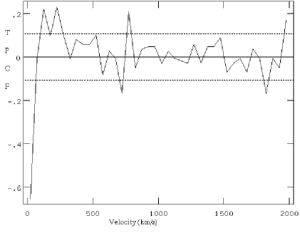
where is the number of observed pairs at separation , and is the number of expected pairs if the lines were randomly distributed along the line of sight. is shown in figure 4. The TPCF shows a deficit of 61 lines pairs with separations below 50 km s-1. As the most likely -value was found to be about 25 km s-1, and a significant number of lines had Doppler widths considerably larger than this, the deficit could entirely be due to line blanketing, where one line obscures another, or line blending, where two lines would be fitted as one. These blended lines could also help explain the non-Gaussian tail in the -distribution. This effect could also lower the observed value of for 50100 km s-1, and so we shall focus on correlations on scales larger than this.
There is only marginal evidence of clustering along the line of sight over the velocity range 100250 km s-1. We find =0.180.06 over this range. There is no evidence for any clustering on scales larger than this. This result is similar to that of Hu et al. (1995) who found 0.170.045 over the range 50150 km s-1. Lu et al. (1996b) also noted a weak, statistically marginal, clustering signal over a similar velocity range. Cristiani et al. (1997) found a small but significant signal at 100 km s-1 of =0.20.04. Further analysis showed that the signal was due to strong clustering in the larger Ly clouds, and that lines with (H I)cm-2 showed no evidence for clustering. Crotts (1989), Chernomordik (1995), and Hu et al. (1995) have also noted a stronger correlation with larger clouds. Kirkman & Tytler (1997), however, found no signal on any scale, with =0.060.045 in the range 50150 km s-1.
Cen et al. (1997) analysed Ly clouds in simulated spectra, using a CDM model, and predicted a significant positive correlation of =0.1 - 1.0 on separations of 50300 km s-1 at z=3. Due to the finite box size, this is in fact an underestimate of the correlation in these simulations. Our results are in line with the lower end of the prediction, but rule out clustering on a scale 1.0.
4.2 The 1-point and 2-point joint probability distribution

The recent N-body cosmological simulations of the Ly forest (e.g. Cen et al. 1994; Miralda-Escudé et al. 1996) have called into question the physical meaning behind the Voigt profile fitting procedure. In the past, Ly clouds were viewed as discrete clouds confined by pressure or gravity within the intergalactic medium (IGM). If these clouds had a Gaussian velocity dispersion then the Voigt profile would describe the resulting line profile, and the physical column density and Doppler width parameters could be estimated. The new paradigm, brought about by the cosmological simulations, views the Ly forest as fluctuations in the IGM itself. Some of the Ly forest lines in the simulations are seen to be non-Voigt, due to gravitational infall, or flows in the IGM. In the simulation models, the Ly clouds have a variety of shapes and sizes, from nearly spherical clouds, to elongated filamentary structures, and cannot be described by a simple model [Cen and Simcoe 1997].
The Voigt profile analysis also has large intrinsic uncertainties due to line blending seen in high quality, high redshift data. Different initial guesses, and number of lines fitted to a region may determine different local minima in the parameter space [Kirkman & Tytler 1997] This non-uniqueness is not helped by increasing S/N. This has lead to the consideration of other statistics when comparing the observed quasar absorption spectra with those from simulations. Following Miralda-Escudé et al. (1997), we have measured the 1-point, and 2-point joint probability distribution of the transmitted flux in the Ly forest spectrum of GB1759+7539.
The Ly forest region of GB1759+7539 is very rich in heavy element features, with over 30% of the Voigt profiles fitted positively identified as heavy element lines. Heavy element absorption lines tend to be much narrower than Ly lines, due to the lower thermal velocity dispersion of the heavier ions. We have investigated the effect that heavy element contamination has on the flux statistics, to test their discriminatory power.
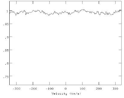
The 1-point and 2-point joint probability distribution of the transmitted flux were calculated on the whole available spectrum, excluding the regions where the damping wings of the two large systems suppressed the spectrum. The results are shown as the solid lines in figures 5 and 6. Then, in order to investigate the effect of the heavy element features, all of the identified heavy element lines were masked off, and the distributions were calculated again. The results for the heavy element-free regions of the spectrum are shown as the dashed lines in figures 5 and 6.
It is clear, from studying figure 5, that the effect of masking out the heavy element lines is to slightly raise the average transmitted flux. This is to be expected, as only regions where heavy element absorption was present were masked off, and not regions where no absorption was seen. The shape of the flux probability distribution, however, appears almost unchanged.

The effect of raising the average transmitted flux when the heavy element lines are masked off also explains the higher levels of the mean flux difference at high velocity separations in the heavy element-free spectrum seen in figure 6. The shape of the 2-point joint probability distribution at separation velocities km s-1 is a good indication of the mean profile of the absorption lines. For , the curve depends on the mean shape of saturated lines, whereas the curve is sensitive to weak absorbers. It can be seen, however, that there is virtually no difference between the two samples, with and without the heavy element lines. This indicates that the statistic does not detect heavy element contamination, or equivalently, it is not a good discriminator between samples where a large minority of lines are drawn from a different, intrinsically narrower distribution, and samples where no such narrow lines are present.
4.3 Departures from the Voigt profile
A clear signature of deviations from Voigt profiles is observed in the simulated forest spectra [Miralda-Escudé et al. 1996], typically in systems still in a collapse phase. The cool, dense gas in its core produces a high column-density, narrow component, whereas the bulk motion, and shock-heating of the infalling material typically produces a broader component [Rauch 1996], producing departures, often asymmetric, from the Voigt profile. Although Voigt profile fitting yields an excellent fit to the data, it is expected that information about this intrinsic non-Voigtness is contained in the way that small, or broad lines cluster about intermediate strength Ly lines.
In order to investigate this, we decided to remove all of the strong Ly lines from the spectrum, leaving just the small clouds that may show some such evidence of clustering. This was achieved by dividing the spectrum of GB1759+7539 by the Voigt profile fits of all heavy element lines, and all the hydrogen lines of Ly forest clouds with a column density (H I)cm-2. All points of the spectrum with a flux level of less than 0.2 times the continuum level were not included in the division, and were then given zero weighting in the following addition. This spectrum should therefore still contain the signature of the small infalling clouds, which would tend to be fitted with Voigt profiles of column density (H I)cm-2, with the central narrow components now removed. Although this signature would be difficult to see in any single system, due to the low S/N and blending effects, it can be searched for statistically by stacking many such systems with the central Ly component removed. If the departures from a Voigt profile were significant, one would expect to see a slight dip in the residual flux either side of the central wavelength in this composite spectrum.
A composite spectrum was formed by shifting the divided spectrum of each system to the rest frame of the removed Ly line, rebinning onto a common velocity scale, and averaging all such rest-frame spectra, using variance weighting. 150 intermediate strength ((H I)cm-2) Ly lines were used, giving a final S/N 400. The composite spectrum can be seen in figure 7.
There is no significant evidence in the composite spectrum (figure 7) of Voigt profile departures due to infalling gas, as described in Miralda-Escudé et al. . The spectrum shows no significant dip either side of the central wavelength, and is consistent with the smaller Ly lines being distributed randomly along the line-of-sight. Different column density limits, both for the summation, and for inclusion in the division were also used, but the results were similarly featureless. Similar tests need to be performed on simulated data to see if this constraint is an important one.
5 The Heavy Element Systems
In the line of sight to GB1759+7539 there are two large systems with conspicuous damping wings, as well as numerous smaller heavy element systems. One of the two systems has a column density (H I); the established, yet somewhat arbitrary criterion for a damped Lyman-alpha system (DLA) [Wolfe et al. 1986]. The other system has a slightly lower column density ((H I)), but displays similar properties to the larger DLAs. In this section we will study the elemental abundances of these two systems. We will only consider those abundance measurements that appear free from saturation effects, and use Fe as the metallicity indicator. The effects of dust on the measured abundances, the ratios of elements produced in different nucleosynthesis processes, and the implications for galactic chemical evolution will be discussed.
5.1 Dust depletion
In the diffuse inter-stellar medium (ISM) clouds, the relative intrinsic abundances are believed to be solar, and so any departures are thought to be due to varying levels of dust depletion [Savage and Sembach 1996]. The refractory elements, with a high condensation temperature, are heavily depleted by the formation of dust grains, whereas the abundance of elements with a low condensation temperature is largely unaffected. Generally, the elements S, P, Zn, C, N, and O are depleted by a factor about 3 or less, but elements Si, Fe, Cr, Al, and Ni are much more heavily depleted in the ISM.
High redshift, young galaxies may have a different chemical enrichment pattern than present day galaxies, due to the different timescales of the various nucleosynthesis processes. In order to objectively study the dust depletion seen in DLAs, one therefore needs to compare the abundances of elements produced in the same nucleosynthesis processes that have very different depletion patterns. Vladilo (1998) studied the abundances of Zn, Fe, and Cr in a sample of 17 DLAs, and concluded that the dust-to-gas ratio was between 2 and 25 % of the Galactic value. This is in good agreement with the value of 5 - 20 % estimated by Pei, Fall & Bechtold (1991) from their study of the reddening of QSOs with foreground DLA absorption. Pettini et al. (1997a) concluded that the “typical” dust-to-gas ratio of DLAs is only of that of the Milky Way. Lu et al. (1996a), however, assert that there is no significant evidence for any dust depletion and that the overabundance of Zn relative to Cr may be intrinsic.
5.2 Nucleosynthesis and abundance ratios
Detailed abundance analysis of the disk and halo stars has provided evidence of the chemical evolution of our Galaxy [McWilliam 1997] The chemical composition of low mass stars has changed little since their formation, and so by studying the abundance ratios in old, low metallicity stars, we can learn about the nucleosynthesis processes that took place when our Galaxy was forming.
The halo stars have an average metallicity of [Fe/H]. They have enhanced [/Fe] ratios (where includes O, Mg, Si, and S) by a factor of about 3 relative to solar [McWilliam 1997] due to the year time delay between -element producing SNII and the first SNIa; the main source of Fe-peak elements [Tinsley 1979]. This over-abundance has also been observed in DLAs [Lu et al. 1996a, Pettini et al. 1995].
The production of odd atomic number elements depends on the neutron excess, which in turn depends on the initial metallicity of the nuclear fuel [Truran & Arnett 1971]. This leads to an under-abundance of odd elements, relative to the even atomic number -elements (e.g. [Al/Si]) at low metallicity. The [Al/Fe] ratio, however, increases slightly with decreasing metallicity in Galactic stars [McWilliam 1997] indicating that Al could be classified as a mild -element phenomenologically despite having an odd number of protons.
Some chemical evolution models also predict that nitrogen may be underabundant relative to oxygen in young high redshift objects, due to the delayed release of primary nitrogen in intermediate mass stars relative to oxygen from high mass stars [Vila-Costas & Edmunds 1993]. This effect, however, has not been convincingly seen in H II regions of nearby heavy element-poor galaxies [Thuan et al. 1995], or in blue compact galaxies [Izotov & Thuan 1999]. It has been investigated in high redshift DLAs by Pettini et al. (1995) and Lipman et al. (1995). Later Lu et al. (1998) found a large scatter in the N/Si ratio, so giving support for the time-delay model of primary N production.
5.3 The Damped Ly System at
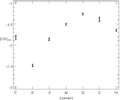
The measured abundances for the DLA are listed in table 2, and plotted in figure 8. The velocity profiles of many of the absorption features can be seen in figure 1. In calculating the abundances, it was assumed that the ion species observed were from the dominant ionization stages in H I gas, so that corrections for other ionization stages are negligible. Given the large H I column density of the system, this is believed to be a good assumption [Viegas 1995]. Also, it is assumed that the H I column density is a good measure of the hydrogen content of the system, since the fraction of molecular hydrogen is known to be small [Levshakov et al. 1992].
Another source of uncertainty is that, as seen in the velocity profile of the heavy element lines, there are several components contributing to this system. In the H I feature, however, this structure is not seen, and it is possible that there may be a metallicity gradient, or additional components contributing to the Ly line, but not the heavy element lines. We summed the column densities for the heavy element lines over all the components, and so are examining the average properties of the DLA. Although the metallicity may vary through the object, it appears, by comparing the column density of individual heavy element line components, that the relative abundances are fairly constant. The solar abundance values used in the calculation were taken from Anders & Grevesse (1989).
From the abundance of iron, [Fe/H], calculated using the unsaturated line, we observe that the DLA has a metallicity , which is about typical for a DLA at this redshift (Pettini et al. 1997b). Hence, this galaxy is still in the early stages of its chemical evolution. Note, however, that in reaching this conclusion, it is assumed that there is little depletion of Fe onto dust grains. If much dust is present, the system would have a higher metallicity than estimated.
5.4 The System at
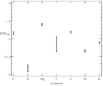
The heavy element system at has a hydrogen column density of Log N(H I)=19.8. The heavy element abundances were calculated as described above, assuming no ionization correction. Due to the smaller size, and lower metallicity of this system, different ion species were on the linear regime of the curve of growth, and hence the calculated abundances are for different species than the system. Only the central component of the weak Fe II feature is seen (see figure 2), so to produce fair relative abundance estimates, only the corresponding components of the other elements were considered. Ignoring the weaker outlying components may lead to an underestimate of the absolute abundances, and hence the overall metallicity of the system, by about 0.1 dex. The measured abundances are listed in table 3, and plotted in figure 9. Assuming little dust depletion, the metallicity of this system is . The velocity profiles of many of the absorption features can be seen in figure 2.
5.4.1 Deuterium Abundance Determination?
Burles & Tytler [Burles and Tytler 1998] attempted to determine the cosmologically important D/H ratio by observing the Ly, Ly, and Ly absorption line profiles of this system. They claim to have measured a value of Log(D/H). On the basis of the evidence presented here it is hard to see how this measurement could be reliable. Due to the high column density (Log (H I)=19.8) of the system, the hydrogen Ly line (see figure 2), and to some extent the Ly line, obscure the deuterium counterpart at km s-1. Several more Lyman series lines would be required to determine the intrinsic structure in the hydrogen absorption of the system, and distinguish this from any deuterium absorption, and any intervening Ly features. The structure seen in the heavy element absorption lines of the system (7 components of Si II were fitted, spanning over 150 km s-1; see figure 2) suggests that even then an accurate determination may not be possible. Unfortunately, they published only the result, and not the full analysis.
5.5 Discussion: Dust and the intrinsic abundances
The over-abundances of sulphur relative to iron in the two systems, [S/Fe], and [S/Fe] and silicon in the system, [Si/Fe] are consistent with that seen in -elements at this metallicity [McWilliam 1997]. As sulphur is undepleted by the formation of dust grains, yet silicon is heavily depleted, the measurements for the system imply that there must be a low level of dust depletion in this system.
The relative abundance of carbon, [C/Fe], in the smaller system has an essentially solar value. Wheeler et al. (1989) concluded that the abundance of carbon is essentially solar, irrespective of metallicity. A slight enhancement of C was observed in the Galactic disk at low metallicity [Tomkin et al. 1995], but this was not seen in halo stars [McWilliam et al. 1995]. The important point is that carbon has not been seen to be under-abundant at any metallicity. Since carbon is relatively undepleted by dust, but iron is, any dust depletion in this system would imply an intrinsic under-abundance of carbon, and so this adds further weight to the conclusion that the level of dust in the system must be very low.
Prochaska & Wolfe (1999) also observed GB1759+7539 using HIRES on the Keck telescope, with a higher wavelength setting, and concentrated on the absorption features of the system as part of a survey of the chemical abundances of several DLAs. They measured the column density of Fe II, also using the unsaturated line, and obtained an abundance of [Fe/H], higher than our measurement by 0.1 dex. Their coverage did not include the Ly forest, and so a less accurate H I column density estimate was used, explaining the larger quoted errors. Ni II was also observed. An abundance of [Ni/H] was obtained using older oscillator strength values. This is 0.1 dex lower than our determination, after correction for the f-values used. The differences are fairly small, and probably due to different model inputs (e.g. the number of Voigt profile components). Their observations are therefore entirely consistent with ours.
Their most interesting measurement is that of Si II, using the unsaturated line. They find [Si/H]; exactly the same as our measurement for [S/H]2.62. These two elements are both -elements, produced in the same nucleosynthesis processes, and yet have very different dust depletion patterns. The fact that they have the same relative abundance therefore implies that this system has a very low dust content. Cr II was observed with an abundance of [Cr/H], entirely consistent with the Ni and Fe measurements. Unfortunately, however, the Zn II feature was blended with sky lines, making an abundance determination uncertain.
Chemical evolution models predict that there should be a large scatter in the values of [N/O] due to the delayed release of primary nitrogen. The O I line is saturated in both systems, so a comparison with S is considered instead. This is based on the assumption that the ratio O/S is essentially solar. We find that [N/S] and [N/S], which is lower than that of the heavy element-poor H II regions, and consistent with the time-delay model of primary nitrogen production.
The abundance of phosphorus was measured at [P/Fe]. In the smaller system, aluminium was observed, with [Al/Fe]. P and Al have an odd number of protons, and so should be under-abundant relative to even atomic number elements. Indeed, [P/S], and [Al/Si] as expected. McWilliam (1997) noted that Na, and Al are have a slight over-abundance relative to Fe at low metallicities. Since P is formed from Al by the addition of an alpha-particle, it too should exhibit the same property. Our measured abundance is consistent with this.
6 The CMB Temperature at
According to Big Bang theory, the temperature of the cosmic microwave background (CMB) should increase linearly with . The local background temperature has been accurately measured at 2.73K. Bahcall & Wolf (1968) suggested that by observing the relative populations of ground-state fine-structure lines of certain atoms, as seen in QSO absorption systems, one could estimate the temperature of the CMB at high redshift. In the last few years, several measurements at high redshift have been made, using the fine-structure levels of C I and C II [Songaila et al. 1994(a), Songaila et al. 1994(b), Lu et al. 1996a, Lu et al. 1996c], all of which were consistent with the Big Bang prediction.
The C II line of the DLA was saturated. Therefore, in order to estimate an upper limit for the temperature of the CMB, we assume that [C/Fe] and hence that log (C II) . The ratio [C/Fe] is believed to be essentially solar at all metallicities [Wheeler et al. 1989], and the effect of any dust would be to increase the intrinsic metallicity, and hence the abundance of C. Therefore, we believe this to be a fair assumption. The velocity profile for the marginally detected C II* absorption feature can be seen in figure 1. Although the profile appears to match that of other low ionization lines (e.g. Ni II) giving confidence in the identification, it lies in the Ly forest, and hence there is the possibility of Ly contamination. Therefore, we take an upper limit (3) of log (C II*) . The C II*/C II ratio then yields an upper limit of TK at . This is very close to the Big Bang cosmology prediction, TK, at this redshift, which suggests that there is negligible excitation of the C II ions by other mechanisms.
7 Summary and Conclusions
We obtained an echelle spectrum of the high-redshift QSO GB1759+7539 () using the instrument HIRES on the Keck 10m telescope. The spectrum has wavelength coverage 4100 - 6540Å, a resolution of FWHM=7 km s-1, and a typical S/N per 2 km s-1 pixel of in the Ly forest region, and longward of the Ly emission. Voigt profiles were fitted to all of the absorption features, and the heavy element lines from twelve heavy element systems were identified. The Ly forest lines, and the absorption features of the two large systems were analysed in detail.
The observed Ly forest systems have a mean redshift of . The H I column density distribution is well described by a power law distribution with index in the range log. The Doppler width distribution is consistent with a Gaussian distribution of mean km s-1, and standard deviation km s-1 with a cut-off at km s-1. There is marginal evidence of clustering along the line of sight over the velocity range 100 km s-1. The 1-point and 2-point joint probability distributions of the transmitted flux in the Ly forest region of the spectrum were calculated, and shown to be very insensitive to the heavy element contamination. We could find no evidence of Voigt profile departures due to infalling gas, as observed in the simulated forest spectra [Miralda-Escudé et al. 1996].
The C, N, O, Al, Si, P, S, Mg, Fe, and Ni absorption features of the large systems were studied, and the elemental abundances calculated for the weak unsaturated lines. The systems have metallicities of and . Both systems appear to have a low dust content. They show an over-abundance of -elements relative to Fe-peak elements, and an under-abundance of odd atomic number elements relative to even. N was found to be under-abundant relative to O, in line with the time delay model of primary N production.
Acknowledgements
We would like to thank Max Pettini, Sandra Savaglio, and an anonymous referee, for helpful comments. PJO acknowledges support from PPARC. Much of the data reduction and analysis was performed on the Starlink-supported computer network at the Institute of Astronomy.
References
- [Anders and Grevesse 1989] Anders, E., Grevesse, N. 1989, Geochim. cosmochim. Acta, 53, 197.
- [Bahcall and Wolf 1968] Bahcall, J.N., Wolf, R.A. 1968, ApJ, 152, 701.
- [Burles and Tytler 1998] Burles, S., Tytler, D. 1998, Space Sci. Rev., 84, 65.
- [Cen et al. 1994] Cen, R., Miralda-Escudé, J., Ostriker, J.P., Rauch, M. 1994, ApJ, 437, 9.
- [Cen et al. 1997] Cen, R., Phelps, S., Miralda-Escudé, J., Ostriker, J.P. 1998, ApJ, 496, 577.
- [Cen and Simcoe 1997] Cen, R., Simcoe, R.A. 1997, ApJ, 483, 8.
- [Chernomordik 1995] Chernomordik, V.V. 1995, ApJ, 440, 431.
- [Condon et al. 1989] Condon, J.J., Broderick J.J., Seielstad, G.A. 1989, AJ, 97, 1064.
- [Cooke 1994] Cooke, A.J. 1994, Ph.D. thesis, Cambridge University.
- [Cristiani et al. 1997] Cristiani, S., D’Odorico, S., D’Odorico, V., Fontana, A., Giallongo, E., Moscardini, L., Savaglio, S. 1997, in Structure and Evolution of the IGM from QSO Absorption Line Systems, eds. P. Petitjean, S. Charlot (Editions Frontières), 165.
- [Crotts 1989] Crotts, A.P.S. 1989, ApJ, 336, 550.
- [Fedchak & Lawler 1999] Fedchak, J.A., Lawler, J.E. 1999, ApJ, submitted.
- [Fitzpatrick 1997] Fitzpatrick, E.L. 1997, ApJ, 482, L99.
- [Haehnelt et al. 1997] Haehnelt, M.G., Steinmetz, M., Rauch, M. 1998, ApJ, 495, 647.
- [Hook et al. 1996] Hook, I.M., McMahon, R.G., Irwin, M.J., Hazard, C. 1996, MNRAS, 282, 1274.
- [Hu et al. 1995] Hu, E.M., Kim, T-S., Cowie, L.L., Songaila, A. 1995, AJ, 110, 1526.
- [Izotov & Thuan 1999] Izotov, Y. I., Thuan, T. X. 1999, to appear in ApJ.
- [Kirkman & Tytler 1997] Kirkman, D., Tytler, D. 1997, ApJ, 484, 672.
- [Lanzetta et al. 1995] Lanzetta, K.M., Wolfe, A.M., Turnshek, D.A. 1995, ApJS, 440, 435.
- [Levshakov et al. 1992] Levshakov, S.A., Chaffee, F.H., Foltz, C.B., Black, J.H. 1992, A&A, 262, 385.
- [Lipman et al. 1995] Lipman, K., Pettini, M., Hunstead, R.W. 1995, in QSO Absorption Lines, ed. G. Meylan (Springer-Verlag), 89.
- [Lu et al. 1996a] Lu, L., Sargent, W.L.W., Barlow, T.A., Churchill, C.W., Vogt, S.S. 1996, ApJS, 107, 475 (a).
- [Lu et al. 1996b] Lu, L., Sargent, W.L.W., Womble, D.S., Takada-Hidai, M. 1996, ApJ, 472, 509 (b).
- [Lu et al. 1996c] Lu, L., Sargent, W.L.W., Womble, D.S., Barlow, T.A. 1996, ApJ, 457, L1 (c).
- [Lu et al. 1998] Lu, L., Sargent, W.L.W., Barlow, T.A. 1998, AJ, 115, 55.
- [McWilliam et al. 1995] McWilliam, A., Preston, G.W., Sneden, C., Shectman, S. 1995, AJ, 109, 2736.
- [McWilliam 1997] McWilliam, A. 1997, ARA&A, 35, 503.
- [Miralda-Escudé et al. 1996] Miralda-Escudé, J., Cen, R., Ostriker, J.P., Rauch, M. 1996, ApJ, 471, 582.
- [Miralda-Escudé et al. 1997] Miralda-Escudé, J., Rauch, M., Sargent, W. L. W., Barlow, T. A., Weinberg, D. H., Hernquist, L., Katz, N., Cen, R., Ostriker J. P. 1997, in Structure and Evolution of the Intergalactic Medium from QSO Absorption Line Systems, ed. P. Petitjean & S. Charlot (Editions Frontieres), 155.
- [Morton 1991] Morton, D.C. 1991, ApJS, 77, 119.
- [Pei et al. 1991] Pei, Y.C., Fall, S.M., Bechtold, J. 1991, ApJ, 378, 6.
- [Petitjean et al. 1993] Petitjean, P., Webb, J.K., Rauch, M., Carswell, R.F., Lanzetta, K. 1993, MNRAS, 262, 499.
- [Pettini et al. 1994] Pettini, M., Smith, L.J., Hunstead, R.W., King, D.L. 1994, ApJ, 426, 79.
- [Pettini et al. 1995] Pettini, M., Lipman, K., Hunstead, R.W. 1995, ApJ, 451, 100.
- [Pettini et al. 1997(a)] Pettini, M., King, D.L., Smith, L.J., Hunstead, R.W. 1997, ApJ, 478, 536 (a).
- [Pettini et al. 1997(b)] Pettini, M., Smith, L.J., King, D.L., Hunstead, R.W. 1997, ApJ, 486, 665 (b).
- [Prochaska & Wolfe 1997] Prochaska, J.X., Wolfe, A.M. 1997, ApJ, 487, 73.
- [Prochaska & Wolfe 1999] Prochaska, J.X., Wolfe, A.M. 1999, ApJS, 121, 369.
- [Rauch et al. 1992] Rauch, M., Carswell, R.F., Chaffee, F.H., Foltz, C.B., Webb, J.K., Weymann, R.J., Bechtold, J., Green, R.F. 1992, ApJ, 390, 387.
- [Rauch 1996] Rauch, M. 1996, in Cold Gas at High Redshift, ed. Bremer, M.N. (Kluwer Academic Publishers).
- [Savage and Sembach 1996] Savage, B.D., Sembach, K.R. 1996, ARA&A, 34, 279.
- [Songaila et al. 1994(a)] Songaila, A., Cowie, L.L., Hogan, C., Rugers, M., 1994, Nature, 368, 599 (a).
- [Songaila et al. 1994(b)] Songaila, A., Cowie, L.L., Vogt, S., Keane, M., Wolfe, A.M., Hu, E.M., Oren, A.L., Tytler, D. R., Lanzetta, K.M. 1994, Nature, 371, 43 (b).
- [Thuan et al. 1995] Thuan, T.X., Izotov, Y.I., Lipovetsky, V.A. 1995, ApJ, 445, 108.
- [Tinsley 1979] Tinsley, B.M. 1979, ApJ, 229, 1046.
- [Tomkin et al. 1995] Tomkin, J., Woolf, V.M., Lambert, D.L. 1995, AJ, 109, 2204.
- [Tripp, Lu, & Savage 1996] Tripp, T.M., Lu, L., Savage, B.D. 1996, ApJS, 102, 239.
- [Truran & Arnett 1971] Truran, J.W., Arnett, W.D. 1971, Astrophys. Space Sci., 11, 430.
- [Viegas 1995] Viegas, S.M. 1995, MNRAS, 276, 268.
- [Vila-Costas & Edmunds 1993] Vila-Costas, M.B., Edmunds, M.G. 1993, MNRAS, 265, 199.
- [Vladilo 1998] Vladilo, G. 1998, ApJ, 493, 583.
- [Vogt 1992] Vogt, S.S. 1992, in High Resolution Spectroscopy with the VLT, ed. M-H Ulrich (Garching: ESO), 223.
- [Webb 1987] Webb, J.K. 1987, Ph.D. thesis, Cambridge University.
- [Wheeler et al. 1989] Wheeler, J.C., Sneden, C., Truran, J.W. 1989, ARA&A, 27, 279.
- [Wolfe 1995] Wolfe, A.M. 1995, in QSO Absorption Lines, ed. G.Meylan (Springer-Verlag), 13.
- [Wolfe et al. 1986] Wolfe, A.M., Turnshek, D.A., Smith, H.A., Cohen, R.D. 1986, ApJSS, 61, 249.
- [Zhang et al. 1995] Zhang, Y., Anninos, P., Norman, M.L. 1995, ApJ, 453, L57.
| ID | Log | |||||||
|---|---|---|---|---|---|---|---|---|
| Si IV | 1402.77 | 4117.27 | 1.935102 | 0.000000 | 8.48 | 0.00 | 12.987 | 0.044 |
| Si IV | 1402.77 | 4117.80 | 1.935480 | 0.000000 | 7.93 | 0.00 | 12.407 | 0.150 |
| Si IV | 1402.77 | 4118.26 | 1.935805 | 0.000000 | 8.76 | 0.00 | 13.034 | 0.056 |
| Si IV | 1402.77 | 4118.72 | 1.936137 | 0.000000 | 5.27 | 0.00 | 12.995 | 0.214 |
| H I | 1215.67 | 4118.82 | 2.388111 | 0.000030 | 12.35 | 2.08 | 13.065 | 0.117 |
| H I | 1215.67 | 4119.53 | 2.388697 | 0.000010 | 19.36 | 1.28 | 13.730 | 0.035 |
| H I | 1215.67 | 4123.34 | 2.391830 | 0.000048 | 33.36 | 6.13 | 13.134 | 0.068 |
| H I | 1215.67 | 4124.61 | 2.392876 | 0.000070 | 25.84 | 9.12 | 12.779 | 0.127 |
| H I | 1215.67 | 4126.21 | 2.394188 | 0.000081 | 28.26 | 10.08 | 12.735 | 0.132 |
| H I | 1215.67 | 4127.48 | 2.395231 | 0.000020 | 25.76 | 2.41 | 13.308 | 0.036 |
| H I | 1215.67 | 4129.54 | 2.396926 | 0.000048 | 21.60 | 6.10 | 12.734 | 0.102 |
| H I | 1215.67 | 4130.46 | 2.397687 | 0.000058 | 17.51 | 7.73 | 12.523 | 0.159 |
| H I | 1215.67 | 4131.52 | 2.398557 | 0.000117 | 36.96 | 15.80 | 12.680 | 0.151 |
| H I | 1215.67 | 4135.61 | 2.401921 | 0.000032 | 9.65 | 4.45 | 12.367 | 0.146 |
| H I | 1025.72 | 4135.94 | 3.032231 | 0.000004 | 24.41 | 0.48 | 13.507 | 0.010 |
| H I | 1215.67 | 4137.08 | 2.403128 | 0.000060 | 40.59 | 7.56 | 12.861 | 0.069 |
| H I | 1215.67 | 4141.37 | 2.406656 | 0.000023 | 48.68 | 2.75 | 13.545 | 0.022 |
| Fe II | 1143.23 | 4143.49 | 2.624384 | 0.000023 | 15.00 | 3.39 | 12.760 | 0.077 |
| Fe II | 1143.23 | 4144.41 | 2.625190 | 0.000003 | 22.47 | 0.29 | 14.785 | 0.008 |
| H I | 1215.67 | 4144.78 | 2.409458 | 0.000064 | 64.63 | 8.15 | 13.338 | 0.048 |
| Fe II | 1143.23 | 4144.94 | 2.625649 | 0.000005 | 6.31 | 1.02 | 14.284 | 0.122 |
| Fe II | 1143.23 | 4145.09 | 2.625782 | 0.000177 | 12.73 | 7.26 | 13.637 | 0.492 |
| Fe II | 1143.23 | 4145.26 | 2.625936 | 0.000005 | 3.26 | 1.28 | 13.256 | 0.156 |
| H I | 1215.67 | 4146.15 | 2.410590 | 0.000027 | 21.77 | 3.61 | 12.907 | 0.059 |
| Si II | 1190.42 | 4146.99 | 2.483654 | 0.000009 | 13.65 | 0.94 | 13.072 | 0.029 |
| Si II | 1190.42 | 4147.24 | 2.483862 | 0.000007 | 4.78 | 1.35 | 12.479 | 0.096 |
| Si II | 1190.42 | 4147.49 | 2.484076 | 0.000003 | 6.96 | 0.40 | 13.032 | 0.016 |
| Fe II | 1144.94 | 4149.70 | 2.624384 | 0.000023 | 15.00 | 3.39 | 12.760 | 0.077 |
| Fe II | 1144.94 | 4150.62 | 2.625190 | 0.000003 | 22.47 | 0.29 | 14.785 | 0.008 |
| Fe II | 1144.94 | 4151.14 | 2.625649 | 0.000005 | 6.31 | 1.02 | 14.284 | 0.122 |
| Fe II | 1144.94 | 4151.30 | 2.625782 | 0.000177 | 12.73 | 7.26 | 13.637 | 0.492 |
| Fe II | 1144.94 | 4151.47 | 2.625936 | 0.000005 | 3.26 | 1.28 | 13.256 | 0.156 |
| H I | 1025.72 | 4151.03 | 3.046940 | 0.000027 | 16.98 | 1.50 | 13.034 | 0.105 |
| H I | 1025.72 | 4151.39 | 3.047284 | 0.000032 | 19.38 | 2.20 | 13.112 | 0.092 |
| H I | 1215.67 | 4153.39 | 2.416549 | 0.000005 | 26.80 | 0.85 | 14.403 | 0.046 |
| H I | 1025.72 | 4153.87 | 3.049704 | 0.000003 | 29.99 | 0.20 | 13.710 | 0.005 |
| Si II | 1193.29 | 4157.00 | 2.483654 | 0.000009 | 13.65 | 0.94 | 13.072 | 0.029 |
| H I | 1215.67 | 4157.15 | 2.419643 | 0.000028 | 11.36 | 3.48 | 12.705 | 0.108 |
| Si II | 1193.29 | 4157.25 | 2.483862 | 0.000007 | 4.78 | 1.35 | 12.479 | 0.096 |
| Si II | 1193.29 | 4157.51 | 2.484076 | 0.000003 | 6.96 | 0.40 | 13.032 | 0.016 |
| H I | 1215.67 | 4159.21 | 2.421338 | 0.000048 | 53.48 | 5.80 | 13.186 | 0.042 |
| H I | 1215.67 | 4163.24 | 2.424646 | 0.000133 | 55.40 | 20.99 | 12.698 | 0.140 |
| H I | 1215.67 | 4165.39 | 2.426421 | 0.000149 | 67.03 | 21.44 | 12.914 | 0.110 |
| H I | 1215.67 | 4166.94 | 2.427693 | 0.000034 | 12.09 | 4.61 | 12.465 | 0.138 |
| H I | 1215.67 | 4168.50 | 2.428980 | 0.000089 | 56.12 | 11.25 | 13.005 | 0.074 |
| H I | 1215.67 | 4170.77 | 2.430846 | 0.000014 | 28.76 | 1.44 | 14.020 | 0.026 |
| H I | 1215.67 | 4171.74 | 2.431646 | 0.000013 | 24.80 | 1.78 | 14.056 | 0.036 |
| H I | 1215.67 | 4173.02 | 2.432695 | 0.000105 | 74.20 | 17.54 | 13.416 | 0.084 |
| H I | 1215.67 | 4174.61 | 2.434004 | 0.000018 | 21.58 | 2.57 | 13.177 | 0.052 |
| H I | 1215.67 | 4175.46 | 2.434698 | 0.000010 | 22.88 | 1.22 | 13.469 | 0.019 |
| P II | 1152.82 | 4179.22 | 2.625222 | 0.000017 | 10.77 | 2.11 | 12.935 | 0.068 |
| H I | 1215.67 | 4180.73 | 2.439041 | 0.000006 | 45.78 | 1.10 | 14.624 | 0.034 |
| H I | 1215.67 | 4186.61 | 2.443875 | 0.000009 | 24.76 | 1.06 | 13.396 | 0.017 |
| H I | 1215.67 | 4188.14 | 2.445136 | 0.000038 | 39.55 | 4.94 | 13.017 | 0.045 |
| H I | 1215.67 | 4189.66 | 2.446382 | 0.000018 | 34.24 | 2.28 | 13.238 | 0.024 |
| H I | 1215.67 | 4191.17 | 2.447628 | 0.000042 | 24.87 | 5.48 | 12.600 | 0.078 |
| H I | 1215.67 | 4192.16 | 2.448438 | 0.000023 | 20.24 | 3.09 | 12.773 | 0.056 |
| H I | 1215.67 | 4193.29 | 2.449366 | 0.000146 | 39.77 | 16.47 | 12.606 | 0.259 |
| H I | 1215.67 | 4194.60 | 2.450448 | 0.000137 | 61.38 | 37.36 | 12.805 | 0.228 |
| H I | 1215.67 | 4195.99 | 2.451590 | 0.000058 | 28.44 | 7.12 | 12.674 | 0.133 |
| Si III | 1206.50 | 4199.36 | 2.480619 | 0.000006 | 8.51 | 0.75 | 12.435 | 0.028 |
| Si III | 1206.50 | 4199.65 | 2.480854 | 0.000006 | 6.34 | 0.78 | 12.293 | 0.034 |
| H I | 1215.67 | 4200.81 | 2.455554 | 0.000023 | 11.25 | 3.09 | 12.340 | 0.091 |
| ID | Log | |||||||
|---|---|---|---|---|---|---|---|---|
| H I | 1215.67 | 4201.59 | 2.456196 | 0.000007 | 20.86 | 0.84 | 13.364 | 0.016 |
| Si III | 1206.50 | 4203.22 | 2.483818 | 0.000025 | 13.50 | 0.79 | 14.224 | 0.295 |
| Si III | 1206.50 | 4203.74 | 2.484244 | 0.000041 | 20.32 | 2.22 | 13.278 | 0.097 |
| H I | 1215.67 | 4207.29 | 2.460888 | 0.000051 | 50.90 | 6.16 | 13.084 | 0.045 |
| H I | 1215.67 | 4209.72 | 2.462880 | 0.000033 | 23.53 | 4.06 | 12.758 | 0.063 |
| H I | 1215.67 | 4211.76 | 2.464566 | 0.000006 | 30.67 | 0.78 | 14.123 | 0.021 |
| H I | 1215.67 | 4214.71 | 2.466985 | 0.000015 | 23.07 | 1.72 | 13.328 | 0.030 |
| H I | 1215.67 | 4217.25 | 2.469076 | 0.000060 | 53.40 | 7.81 | 13.219 | 0.052 |
| H I | 1215.67 | 4219.01 | 2.470529 | 0.000023 | 32.63 | 2.49 | 13.823 | 0.030 |
| H I | 1215.67 | 4219.84 | 2.471210 | 0.000026 | 22.25 | 2.58 | 13.431 | 0.058 |
| H I | 1215.67 | 4229.09 | 2.478820 | 0.000301 | 100.00 | 28.49 | 13.280 | 0.141 |
| H I | 1215.67 | 4231.37 | 2.480691 | 0.000009 | 18.62 | 1.84 | 15.088 | 0.288 |
| H I | 1215.67 | 4232.20 | 2.481372 | 0.000145 | 100.00 | 16.89 | 13.988 | 0.063 |
| H I | 1215.67 | 4234.24 | 2.483056 | 0.000048 | 39.33 | 4.71 | 14.801 | 0.165 |
| H I | 1215.67 | 4236.21 | 2.484674 | 0.000073 | 84.35 | 12.28 | 14.694 | 0.038 |
| H I | 1215.67 | 4238.21 | 2.486319 | 0.000016 | 21.96 | 2.72 | 15.256 | 0.350 |
| H I | 1215.67 | 4239.29 | 2.487205 | 0.000050 | 46.66 | 4.51 | 13.653 | 0.046 |
| H I | 1215.67 | 4244.90 | 2.491824 | 0.000042 | 19.82 | 5.42 | 12.519 | 0.098 |
| H I | 1215.67 | 4250.77 | 2.496646 | 0.000007 | 21.78 | 0.80 | 13.569 | 0.017 |
| H I | 1215.67 | 4252.47 | 2.498043 | 0.000018 | 34.88 | 2.14 | 13.336 | 0.024 |
| H I | 1215.67 | 4254.49 | 2.499703 | 0.000026 | 27.36 | 2.46 | 13.547 | 0.041 |
| H I | 1215.67 | 4255.17 | 2.500261 | 0.000013 | 20.03 | 1.19 | 13.737 | 0.031 |
| H I | 1215.67 | 4257.69 | 2.502333 | 0.000024 | 20.67 | 2.68 | 13.090 | 0.052 |
| H I | 1215.67 | 4258.96 | 2.503379 | 0.000009 | 37.42 | 1.40 | 14.557 | 0.048 |
| H I | 1215.67 | 4268.38 | 2.511126 | 0.000022 | 23.03 | 2.67 | 13.133 | 0.046 |
| H I | 1215.67 | 4269.76 | 2.512266 | 0.000066 | 51.96 | 8.68 | 13.138 | 0.058 |
| H I | 1215.67 | 4273.74 | 2.515535 | 0.000081 | 52.65 | 11.12 | 12.949 | 0.079 |
| H I | 1215.67 | 4282.77 | 2.522968 | 0.000041 | 29.73 | 4.74 | 12.897 | 0.060 |
| H I | 1215.67 | 4284.49 | 2.524385 | 0.000037 | 23.69 | 4.67 | 12.736 | 0.070 |
| H I | 1215.67 | 4285.88 | 2.525523 | 0.000013 | 27.70 | 1.57 | 13.395 | 0.021 |
| H I | 1215.67 | 4287.25 | 2.526649 | 0.000006 | 30.35 | 1.04 | 14.342 | 0.034 |
| H I | 1215.67 | 4288.74 | 2.527875 | 0.000027 | 37.67 | 3.31 | 13.682 | 0.035 |
| H I | 1215.67 | 4289.78 | 2.528730 | 0.000035 | 34.58 | 3.02 | 13.499 | 0.046 |
| H I | 1215.67 | 4294.48 | 2.532599 | 0.000022 | 15.58 | 2.70 | 12.612 | 0.061 |
| H I | 1215.67 | 4295.63 | 2.533542 | 0.000071 | 32.00 | 8.87 | 12.521 | 0.100 |
| H I | 1215.67 | 4297.89 | 2.535407 | 0.000040 | 37.24 | 4.83 | 12.881 | 0.048 |
| H I | 1215.67 | 4301.71 | 2.538543 | 0.000006 | 41.54 | 0.71 | 14.068 | 0.010 |
| H I | 1215.67 | 4305.52 | 2.541685 | 0.000006 | 7.79 | 0.72 | 12.875 | 0.031 |
| H I | 1215.67 | 4308.59 | 2.544209 | 0.000067 | 25.23 | 8.37 | 12.554 | 0.122 |
| H I | 1215.67 | 4309.40 | 2.544876 | 0.000043 | 21.98 | 5.87 | 12.668 | 0.094 |
| Si II | 1190.42 | 4314.51 | 2.624365 | 0.000003 | 10.63 | 0.28 | 13.410 | 0.012 |
| Si II | 1190.42 | 4314.81 | 2.624617 | 0.000003 | 3.27 | 0.33 | 13.076 | 0.025 |
| H I | 1215.67 | 4315.23 | 2.549668 | 0.000061 | 58.07 | 3.40 | 13.940 | 0.075 |
| Si II | 1190.42 | 4315.59 | 2.625274 | 0.000007 | 16.77 | 0.28 | 16.655 | 0.040 |
| Si II | 1190.42 | 4316.31 | 2.625883 | 0.000009 | 9.60 | 0.57 | 14.167 | 0.040 |
| Si II | 1190.42 | 4316.70 | 2.626211 | 0.000009 | 8.58 | 1.01 | 12.602 | 0.046 |
| H I | 1215.67 | 4318.67 | 2.552497 | 0.000011 | 23.42 | 1.32 | 13.497 | 0.026 |
| H I | 1215.67 | 4319.78 | 2.553408 | 0.000053 | 73.41 | 30.83 | 12.815 | 0.160 |
| H I | 1215.67 | 4321.62 | 2.554927 | 0.000012 | 6.80 | 1.63 | 12.616 | 0.073 |
| H I | 1215.67 | 4322.77 | 2.555873 | 0.000077 | 34.34 | 9.37 | 12.734 | 0.101 |
| H I | 1215.67 | 4323.90 | 2.556799 | 0.000041 | 9.23 | 5.38 | 12.206 | 0.188 |
| Si II | 1193.29 | 4324.92 | 2.624365 | 0.000003 | 10.63 | 0.28 | 13.410 | 0.012 |
| Si II | 1193.29 | 4325.22 | 2.624617 | 0.000003 | 3.27 | 0.33 | 13.076 | 0.025 |
| Si II | 1193.29 | 4326.01 | 2.625274 | 0.000007 | 16.77 | 0.28 | 16.655 | 0.040 |
| Si II | 1193.29 | 4326.73 | 2.625883 | 0.000009 | 9.60 | 0.57 | 14.167 | 0.040 |
| Si II | 1193.29 | 4327.12 | 2.626211 | 0.000009 | 8.58 | 1.01 | 12.602 | 0.046 |
| H I | 1215.67 | 4327.67 | 2.559904 | 0.000047 | 17.53 | 5.85 | 12.485 | 0.122 |
| H I | 1215.67 | 4333.49 | 2.564688 | 0.000029 | 22.84 | 3.53 | 12.833 | 0.056 |
| H I | 1215.67 | 4336.43 | 2.567108 | 0.000006 | 21.76 | 0.62 | 13.805 | 0.018 |
| H I | 1215.67 | 4339.68 | 2.569779 | 0.000004 | 32.74 | 0.85 | 14.968 | 0.061 |
| H I | 1215.67 | 4344.23 | 2.573525 | 0.000020 | 9.78 | 2.56 | 12.446 | 0.094 |
| H I | 1215.67 | 4344.91 | 2.574084 | 0.000007 | 24.55 | 0.83 | 13.643 | 0.013 |
| H I | 1215.67 | 4347.31 | 2.576061 | 0.000040 | 45.92 | 5.05 | 13.117 | 0.040 |
| ID | Log | |||||||
|---|---|---|---|---|---|---|---|---|
| N I | 1199.55 | 4348.59 | 2.625185 | 0.000013 | 19.12 | 1.51 | 14.704 | 0.072 |
| N I | 1199.55 | 4348.82 | 2.625376 | 0.000041 | 33.77 | 2.34 | 14.387 | 0.153 |
| N I | 1199.55 | 4349.12 | 2.625624 | 0.000006 | 7.64 | 0.74 | 14.318 | 0.050 |
| N I | 1200.22 | 4351.04 | 2.625185 | 0.000013 | 19.12 | 1.51 | 14.704 | 0.072 |
| N I | 1200.22 | 4351.27 | 2.625376 | 0.000041 | 33.77 | 2.34 | 14.387 | 0.153 |
| N I | 1200.22 | 4351.56 | 2.625624 | 0.000006 | 7.64 | 0.74 | 14.318 | 0.050 |
| H I | 1215.67 | 4352.60 | 2.580412 | 0.000021 | 36.93 | 1.71 | 13.831 | 0.032 |
| N I | 1200.71 | 4352.80 | 2.625185 | 0.000013 | 19.12 | 1.51 | 14.704 | 0.072 |
| N I | 1200.71 | 4353.03 | 2.625376 | 0.000041 | 33.77 | 2.34 | 14.387 | 0.153 |
| N I | 1200.71 | 4353.33 | 2.625624 | 0.000006 | 7.64 | 0.74 | 14.318 | 0.050 |
| H I | 1215.67 | 4356.04 | 2.583239 | 0.000044 | 74.97 | 4.55 | 13.522 | 0.031 |
| H I | 1215.67 | 4356.39 | 2.583530 | 0.000016 | 19.35 | 2.33 | 13.071 | 0.063 |
| H I | 1215.67 | 4359.51 | 2.586095 | 0.000088 | 100.00 | 12.36 | 13.238 | 0.049 |
| H I | 1215.67 | 4363.89 | 2.589694 | 0.000106 | 100.00 | 14.81 | 13.161 | 0.059 |
| H I | 1215.67 | 4366.49 | 2.591832 | 0.000012 | 29.51 | 1.41 | 13.449 | 0.020 |
| H I | 1215.67 | 4368.80 | 2.593736 | 0.000098 | 94.39 | 12.32 | 13.310 | 0.051 |
| Si III | 1206.50 | 4369.47 | 2.621601 | 0.000007 | 8.18 | 0.78 | 12.466 | 0.035 |
| H I | 1215.67 | 4372.33 | 2.596643 | 0.000244 | 26.50 | 16.01 | 12.760 | 0.483 |
| Si III | 1206.50 | 4372.66 | 2.624248 | 0.000012 | 4.97 | 2.14 | 13.591 | 0.921 |
| Si III | 1206.50 | 4373.77 | 2.625171 | 0.000023 | 40.88 | 10.62 | 14.370 | 0.319 |
| Si III | 1206.50 | 4375.01 | 2.626200 | 0.000016 | 9.76 | 1.69 | 14.128 | 0.387 |
| H I | 1215.67 | 4377.77 | 2.601116 | 0.000019 | 14.87 | 2.28 | 12.932 | 0.057 |
| H I | 1215.67 | 4381.85 | 2.604468 | 0.000011 | 38.78 | 1.40 | 14.296 | 0.030 |
| H I | 1215.67 | 4383.41 | 2.605754 | 0.000028 | 32.69 | 4.01 | 13.365 | 0.041 |
| H I | 1215.67 | 4384.67 | 2.606787 | 0.000008 | 23.10 | 1.31 | 14.277 | 0.071 |
| H I | 1215.67 | 4387.39 | 2.609027 | 0.000085 | 54.05 | 10.47 | 13.153 | 0.083 |
| H I | 1215.67 | 4389.35 | 2.610643 | 0.000044 | 13.70 | 5.54 | 12.595 | 0.138 |
| H I | 1215.67 | 4390.36 | 2.611472 | 0.000016 | 17.13 | 1.69 | 13.687 | 0.049 |
| Si II | 1260.42 | 4390.88 | 2.483654 | 0.000009 | 13.65 | 0.94 | 13.072 | 0.029 |
| Si II | 1260.42 | 4391.14 | 2.483862 | 0.000007 | 4.78 | 1.35 | 12.479 | 0.096 |
| Si II | 1260.42 | 4391.41 | 2.484076 | 0.000003 | 6.96 | 0.40 | 13.032 | 0.016 |
| H I | 1215.67 | 4393.48 | 2.614033 | 0.000017 | 24.21 | 2.38 | 14.146 | 0.103 |
| H I | 1215.67 | 4407.51 | 2.625579 | 0.000049 | 78.50 | 46.63 | 20.761 | 0.007 |
| H I | 1215.67 | 4425.57 | 2.640430 | 0.000039 | 14.96 | 4.62 | 12.802 | 0.113 |
| H I | 1215.67 | 4428.98 | 2.643236 | 0.000047 | 19.01 | 5.62 | 12.739 | 0.110 |
| H I | 1215.67 | 4431.24 | 2.645099 | 0.000016 | 22.89 | 1.85 | 13.374 | 0.033 |
| H I | 1215.67 | 4433.34 | 2.646828 | 0.000060 | 57.20 | 7.06 | 13.267 | 0.049 |
| H I | 1215.67 | 4436.10 | 2.649093 | 0.000063 | 40.77 | 7.51 | 12.902 | 0.072 |
| H I | 1215.67 | 4439.03 | 2.651502 | 0.000052 | 64.59 | 5.54 | 13.415 | 0.039 |
| H I | 1215.67 | 4440.79 | 2.652952 | 0.000080 | 24.28 | 13.30 | 12.479 | 0.348 |
| H I | 1215.67 | 4441.98 | 2.653930 | 0.000302 | 100.00 | 29.02 | 13.158 | 0.135 |
| H I | 1215.67 | 4445.36 | 2.656714 | 0.000069 | 37.86 | 8.71 | 12.693 | 0.087 |
| H I | 1215.67 | 4447.41 | 2.658396 | 0.000095 | 47.04 | 12.19 | 12.662 | 0.100 |
| H I | 1215.67 | 4449.50 | 2.660116 | 0.000078 | 48.30 | 9.62 | 12.850 | 0.083 |
| H I | 1215.67 | 4452.20 | 2.662337 | 0.000149 | 100.00 | 25.36 | 12.995 | 0.091 |
| H I | 1215.67 | 4454.48 | 2.664216 | 0.000016 | 14.11 | 2.10 | 13.332 | 0.086 |
| H I | 1215.67 | 4454.69 | 2.664383 | 0.000013 | 38.57 | 1.26 | 13.875 | 0.023 |
| H I | 1215.67 | 4456.40 | 2.665794 | 0.000049 | 43.14 | 7.70 | 12.926 | 0.062 |
| H I | 1215.67 | 4457.79 | 2.666937 | 0.000054 | 29.58 | 7.43 | 12.631 | 0.094 |
| H I | 1215.67 | 4459.12 | 2.668033 | 0.000016 | 30.80 | 1.75 | 13.550 | 0.022 |
| H I | 1215.67 | 4460.01 | 2.668760 | 0.000087 | 26.55 | 13.00 | 12.622 | 0.286 |
| H I | 1215.67 | 4461.30 | 2.669828 | 0.000011 | 23.93 | 2.00 | 13.310 | 0.055 |
| H I | 1215.67 | 4462.13 | 2.670511 | 0.000315 | 100.00 | 29.25 | 13.169 | 0.154 |
| H I | 1215.67 | 4463.87 | 2.671936 | 0.000025 | 13.83 | 3.57 | 12.427 | 0.112 |
| H I | 1215.67 | 4465.44 | 2.673230 | 0.000023 | 20.58 | 2.78 | 12.819 | 0.048 |
| C IV | 1548.20 | 4466.27 | 1.884823 | 0.000002 | 5.23 | 0.30 | 13.851 | 0.044 |
| H I | 1215.67 | 4466.60 | 2.674188 | 0.000046 | 29.62 | 4.22 | 12.945 | 0.065 |
| C IV | 1550.77 | 4473.70 | 1.884823 | 0.000002 | 5.23 | 0.30 | 13.851 | 0.044 |
| Fe II | 1144.94 | 4476.93 | 2.910193 | 0.000003 | 10.10 | 0.28 | 13.658 | 0.010 |
| H I | 1215.67 | 4477.15 | 2.682861 | 0.000072 | 44.64 | 7.38 | 13.220 | 0.048 |
| H I | 1215.67 | 4478.39 | 2.683881 | 0.000072 | 35.44 | 7.04 | 12.968 | 0.098 |
| H I | 1215.67 | 4480.43 | 2.685562 | 0.000065 | 32.17 | 8.31 | 12.665 | 0.089 |
| Si II | 1526.71 | 4481.13 | 1.935161 | 0.000005 | 1.66 | 2.06 | 13.059 | 0.179 |
| ID | Log | |||||||
|---|---|---|---|---|---|---|---|---|
| Si II | 1526.71 | 4481.28 | 1.935259 | 0.000034 | 11.16 | 3.95 | 13.086 | 0.161 |
| H I | 1215.67 | 4483.04 | 2.687711 | 0.000161 | 78.46 | 23.65 | 12.863 | 0.100 |
| H I | 1215.67 | 4485.30 | 2.689567 | 0.000045 | 21.08 | 3.30 | 13.850 | 0.130 |
| H I | 1215.67 | 4485.92 | 2.690076 | 0.000025 | 53.35 | 1.26 | 14.325 | 0.030 |
| H I | 1215.67 | 4488.50 | 2.692196 | 0.000062 | 34.84 | 6.63 | 13.230 | 0.083 |
| H I | 1215.67 | 4489.50 | 2.693025 | 0.000040 | 26.24 | 3.18 | 14.058 | 0.076 |
| N V | 1238.82 | 4490.14 | 2.624522 | 0.000007 | 6.64 | 0.90 | 13.246 | 0.039 |
| H I | 1215.67 | 4490.47 | 2.693822 | 0.000036 | 30.94 | 1.64 | 14.509 | 0.076 |
| N V | 1238.82 | 4491.94 | 2.625976 | 0.000026 | 14.29 | 3.23 | 12.827 | 0.085 |
| H I | 1215.67 | 4493.46 | 2.696279 | 0.000068 | 63.01 | 9.53 | 12.985 | 0.051 |
| Mg II | 1239.93 | 4495.10 | 2.625286 | 0.000016 | 26.73 | 3.17 | 15.502 | 0.082 |
| Mg II | 1239.93 | 4495.55 | 2.625646 | 0.000003 | 8.28 | 0.62 | 15.319 | 0.091 |
| H I | 1215.67 | 4495.89 | 2.698284 | 0.000011 | 28.41 | 1.22 | 13.584 | 0.018 |
| Mg II | 1240.40 | 4496.80 | 2.625286 | 0.000016 | 26.73 | 3.17 | 15.502 | 0.082 |
| Mg II | 1240.40 | 4497.25 | 2.625646 | 0.000003 | 8.28 | 0.62 | 15.319 | 0.091 |
| H I | 1215.67 | 4498.31 | 2.700265 | 0.000016 | 31.99 | 1.97 | 13.193 | 0.025 |
| H I | 1215.67 | 4500.06 | 2.701707 | 0.000037 | 26.43 | 6.39 | 12.677 | 0.153 |
| H I | 1215.67 | 4501.11 | 2.702570 | 0.000158 | 100.00 | 14.04 | 13.217 | 0.069 |
| H I | 1215.67 | 4503.10 | 2.704212 | 0.000037 | 12.88 | 4.92 | 12.134 | 0.150 |
| N V | 1242.80 | 4504.57 | 2.624522 | 0.000007 | 6.64 | 0.90 | 13.246 | 0.039 |
| N V | 1242.80 | 4506.38 | 2.625976 | 0.000026 | 14.29 | 3.23 | 12.827 | 0.085 |
| H I | 1215.67 | 4509.44 | 2.709421 | 0.000004 | 38.40 | 0.78 | 15.040 | 0.048 |
| H I | 1215.67 | 4512.95 | 2.712308 | 0.000022 | 35.05 | 2.58 | 13.013 | 0.027 |
| H I | 1215.67 | 4514.16 | 2.713305 | 0.000011 | 13.99 | 1.63 | 13.035 | 0.088 |
| H I | 1215.67 | 4514.78 | 2.713818 | 0.000019 | 35.26 | 2.51 | 13.665 | 0.027 |
| H I | 1215.67 | 4516.55 | 2.715271 | 0.000004 | 37.27 | 0.91 | 14.805 | 0.039 |
| H I | 1215.67 | 4518.45 | 2.716834 | 0.000010 | 38.43 | 1.31 | 13.537 | 0.012 |
| H I | 1215.67 | 4520.13 | 2.718220 | 0.000014 | 35.32 | 1.90 | 13.327 | 0.031 |
| H I | 1215.67 | 4522.04 | 2.719789 | 0.000158 | 100.00 | 25.88 | 13.025 | 0.089 |
| H I | 1215.67 | 4525.26 | 2.722435 | 0.000110 | 65.97 | 14.82 | 12.824 | 0.089 |
| H I | 1215.67 | 4528.79 | 2.725343 | 0.000281 | 100.00 | 23.54 | 13.412 | 0.123 |
| H I | 1215.67 | 4530.20 | 2.726498 | 0.000008 | 36.73 | 1.30 | 14.321 | 0.022 |
| H I | 1215.67 | 4531.81 | 2.727829 | 0.000133 | 46.96 | 15.03 | 12.666 | 0.138 |
| S II | 1250.58 | 4533.73 | 2.625284 | 0.000007 | 17.78 | 0.91 | 14.992 | 0.022 |
| S II | 1250.58 | 4534.16 | 2.625633 | 0.000006 | 6.68 | 0.75 | 14.673 | 0.053 |
| S II | 1250.58 | 4534.40 | 2.625820 | 0.000039 | 10.48 | 3.69 | 14.093 | 0.173 |
| O I | 1302.17 | 4536.31 | 2.483654 | 0.000000 | 18.09 | 0.00 | 13.698 | 0.040 |
| O I | 1302.17 | 4536.86 | 2.484076 | 0.000000 | 9.22 | 0.00 | 12.903 | 0.160 |
| H I | 1215.67 | 4538.76 | 2.733545 | 0.000008 | 26.15 | 0.86 | 13.853 | 0.014 |
| H I | 1215.67 | 4539.61 | 2.734239 | 0.000013 | 18.92 | 1.32 | 13.316 | 0.028 |
| C IV | 1548.20 | 4541.89 | 1.933663 | 0.000005 | 8.01 | 0.77 | 13.064 | 0.033 |
| H I | 1215.67 | 4543.60 | 2.737520 | 0.000728 | 77.36 | 58.69 | 12.841 | 0.411 |
| Si II | 1304.37 | 4543.98 | 2.483654 | 0.000009 | 13.65 | 0.94 | 13.072 | 0.029 |
| C IV | 1548.19 | 4544.11 | 1.935102 | 0.000004 | 12.96 | 0.83 | 13.706 | 0.037 |
| Si II | 1304.37 | 4544.25 | 2.483862 | 0.000007 | 4.78 | 1.35 | 12.479 | 0.096 |
| Si II | 1304.37 | 4544.53 | 2.484076 | 0.000003 | 6.96 | 0.40 | 13.032 | 0.016 |
| C IV | 1548.20 | 4544.70 | 1.935480 | 0.000009 | 12.12 | 1.87 | 13.258 | 0.096 |
| C IV | 1548.20 | 4545.20 | 1.935805 | 0.000007 | 13.40 | 1.17 | 13.562 | 0.048 |
| S II | 1253.81 | 4545.42 | 2.625284 | 0.000007 | 17.78 | 0.91 | 14.992 | 0.022 |
| C IV | 1548.20 | 4545.72 | 1.936137 | 0.000005 | 8.05 | 0.86 | 13.437 | 0.048 |
| S II | 1253.81 | 4545.86 | 2.625633 | 0.000006 | 6.68 | 0.75 | 14.673 | 0.053 |
| S II | 1253.81 | 4546.10 | 2.625820 | 0.000039 | 10.48 | 3.69 | 14.093 | 0.173 |
| C IV | 1548.20 | 4546.88 | 1.936890 | 0.000008 | 6.05 | 1.45 | 12.637 | 0.070 |
| C IV | 1550.77 | 4549.44 | 1.933663 | 0.000005 | 8.01 | 0.77 | 13.064 | 0.033 |
| H I | 1215.67 | 4551.32 | 2.743878 | 0.000025 | 37.42 | 1.16 | 14.784 | 0.058 |
| C IV | 1550.77 | 4551.67 | 1.935102 | 0.000004 | 12.96 | 0.83 | 13.706 | 0.037 |
| C IV | 1550.77 | 4552.26 | 1.935480 | 0.000009 | 12.12 | 1.87 | 13.258 | 0.096 |
| H I | 1215.67 | 4552.56 | 2.744891 | 0.000127 | 47.28 | 26.75 | 13.676 | 0.414 |
| C IV | 1550.77 | 4552.76 | 1.935805 | 0.000007 | 13.40 | 1.17 | 13.562 | 0.048 |
| C IV | 1550.77 | 4553.28 | 1.936137 | 0.000005 | 8.05 | 0.86 | 13.437 | 0.048 |
| H I | 1215.67 | 4553.74 | 2.745866 | 0.001025 | 66.64 | 58.89 | 13.222 | 0.721 |
| C IV | 1550.77 | 4554.44 | 1.936890 | 0.000008 | 6.05 | 1.45 | 12.637 | 0.070 |
| H I | 1215.67 | 4554.72 | 2.746675 | 0.000028 | 16.94 | 5.21 | 12.671 | 0.211 |
| ID | Log | |||||||
|---|---|---|---|---|---|---|---|---|
| H I | 1215.67 | 4555.48 | 2.747295 | 0.000030 | 8.99 | 5.44 | 12.065 | 0.286 |
| H I | 1215.67 | 4556.82 | 2.748399 | 0.000009 | 24.56 | 1.02 | 13.374 | 0.020 |
| H I | 1215.67 | 4558.45 | 2.749737 | 0.000050 | 70.61 | 4.54 | 13.675 | 0.031 |
| H I | 1215.67 | 4558.90 | 2.750113 | 0.000010 | 12.46 | 1.00 | 13.333 | 0.044 |
| H I | 1215.67 | 4559.37 | 2.750500 | 0.000056 | 22.11 | 6.56 | 12.911 | 0.171 |
| H I | 1215.67 | 4560.90 | 2.751753 | 0.000003 | 20.84 | 0.41 | 13.904 | 0.012 |
| H I | 1215.67 | 4563.09 | 2.753555 | 0.000120 | 100.00 | 19.56 | 13.040 | 0.064 |
| H I | 1215.67 | 4564.74 | 2.754910 | 0.000004 | 2.09 | 0.74 | 12.770 | 0.095 |
| H I | 1215.67 | 4565.32 | 2.755393 | 0.000006 | 25.99 | 0.81 | 13.910 | 0.011 |
| S II | 1259.52 | 4566.12 | 2.625284 | 0.000007 | 17.78 | 0.91 | 14.992 | 0.022 |
| S II | 1259.52 | 4566.56 | 2.625633 | 0.000006 | 6.68 | 0.75 | 14.673 | 0.053 |
| H I | 1215.67 | 4566.73 | 2.756550 | 0.000044 | 37.13 | 3.38 | 13.369 | 0.049 |
| S II | 1259.52 | 4566.79 | 2.625820 | 0.000039 | 10.48 | 3.69 | 14.093 | 0.173 |
| Si II | 1260.42 | 4568.23 | 2.624365 | 0.000003 | 10.63 | 0.28 | 13.410 | 0.012 |
| Si II | 1260.42 | 4568.55 | 2.624617 | 0.000003 | 3.27 | 0.33 | 13.076 | 0.025 |
| Si II | 1260.42 | 4569.38 | 2.625274 | 0.000007 | 16.77 | 0.28 | 16.655 | 0.040 |
| Si II | 1260.42 | 4570.15 | 2.625883 | 0.000009 | 9.60 | 0.57 | 14.167 | 0.040 |
| Si II | 1260.42 | 4570.56 | 2.626211 | 0.000009 | 8.58 | 1.01 | 12.602 | 0.046 |
| H I | 1215.67 | 4571.89 | 2.760796 | 0.000008 | 33.70 | 0.94 | 13.558 | 0.010 |
| H I | 1215.67 | 4573.22 | 2.761886 | 0.000011 | 33.04 | 1.27 | 13.374 | 0.014 |
| H I | 1215.67 | 4576.39 | 2.764499 | 0.000175 | 98.17 | 20.89 | 13.046 | 0.089 |
| H I | 1215.67 | 4579.60 | 2.767135 | 0.000081 | 96.57 | 14.68 | 13.427 | 0.062 |
| H I | 1215.67 | 4581.01 | 2.768299 | 0.000018 | 24.13 | 2.93 | 12.933 | 0.074 |
| H I | 1215.67 | 4583.43 | 2.770287 | 0.000048 | 100.00 | 5.74 | 13.488 | 0.021 |
| H I | 1215.67 | 4587.06 | 2.773273 | 0.000012 | 37.74 | 1.36 | 13.356 | 0.014 |
| H I | 1215.67 | 4590.84 | 2.776380 | 0.000176 | 100.00 | 14.30 | 13.360 | 0.073 |
| H I | 1215.67 | 4592.24 | 2.777534 | 0.000004 | 28.48 | 0.88 | 14.566 | 0.041 |
| H I | 1215.67 | 4593.76 | 2.778787 | 0.000011 | 18.93 | 1.36 | 13.132 | 0.027 |
| H I | 1215.67 | 4594.54 | 2.779425 | 0.000031 | 17.23 | 4.20 | 12.671 | 0.090 |
| H I | 1215.67 | 4595.43 | 2.780159 | 0.000006 | 25.86 | 0.73 | 14.016 | 0.015 |
| H I | 1215.67 | 4596.61 | 2.781132 | 0.000048 | 22.44 | 6.88 | 12.429 | 0.106 |
| H I | 1215.67 | 4602.52 | 2.785990 | 0.000017 | 44.32 | 1.69 | 13.770 | 0.015 |
| H I | 1215.67 | 4603.92 | 2.787142 | 0.000006 | 28.33 | 0.85 | 14.527 | 0.042 |
| H I | 1215.67 | 4608.80 | 2.791154 | 0.000048 | 29.18 | 5.67 | 12.592 | 0.069 |
| H I | 1215.67 | 4610.29 | 2.792382 | 0.000050 | 33.26 | 4.98 | 12.948 | 0.091 |
| H I | 1215.67 | 4612.09 | 2.793865 | 0.000339 | 59.49 | 18.90 | 13.818 | 0.272 |
| H I | 1215.67 | 4613.78 | 2.795255 | 0.000019 | 46.91 | 1.36 | 16.186 | 0.101 |
| H I | 1215.67 | 4616.62 | 2.797589 | 0.000070 | 43.92 | 9.37 | 13.028 | 0.082 |
| H I | 1215.67 | 4617.54 | 2.798348 | 0.000006 | 21.57 | 0.57 | 13.750 | 0.015 |
| H I | 1215.67 | 4622.08 | 2.802077 | 0.000052 | 59.83 | 6.30 | 12.915 | 0.037 |
| H I | 1215.67 | 4623.76 | 2.803462 | 0.000004 | 21.64 | 0.41 | 13.617 | 0.008 |
| H I | 1215.67 | 4626.44 | 2.805671 | 0.000007 | 15.54 | 0.82 | 12.911 | 0.019 |
| H I | 1215.67 | 4632.63 | 2.810756 | 0.000017 | 24.98 | 1.94 | 12.793 | 0.029 |
| H I | 1215.67 | 4634.24 | 2.812082 | 0.000008 | 22.85 | 0.90 | 13.097 | 0.015 |
| H I | 1215.67 | 4638.98 | 2.815980 | 0.000055 | 37.55 | 6.05 | 12.787 | 0.063 |
| Si III | 1206.50 | 4640.16 | 2.845968 | 0.000009 | 12.75 | 1.21 | 12.484 | 0.063 |
| Si III | 1206.50 | 4640.61 | 2.846340 | 0.000043 | 44.16 | 4.73 | 12.776 | 0.052 |
| Si III | 1206.50 | 4640.67 | 2.846386 | 0.000009 | 8.34 | 1.60 | 12.156 | 0.103 |
| Si III | 1206.50 | 4641.87 | 2.847381 | 0.000002 | 5.59 | 0.33 | 12.848 | 0.036 |
| Si III | 1206.50 | 4642.24 | 2.847690 | 0.000064 | 33.73 | 5.54 | 12.258 | 0.077 |
| Si III | 1206.50 | 4644.01 | 2.849158 | 0.000017 | 5.23 | 2.63 | 11.465 | 0.146 |
| Si III | 1206.50 | 4644.56 | 2.849617 | 0.000012 | 4.61 | 0.54 | 15.786 | 0.032 |
| Si III | 1206.50 | 4644.89 | 2.849887 | 0.000017 | 6.25 | 1.29 | 12.748 | 0.101 |
| H I | 1215.67 | 4646.17 | 2.821894 | 0.000034 | 35.12 | 4.19 | 12.854 | 0.042 |
| H I | 1215.67 | 4647.89 | 2.823315 | 0.000016 | 34.95 | 1.90 | 13.136 | 0.019 |
| C II | 1334.53 | 4649.10 | 2.483693 | 0.000014 | 15.95 | 2.10 | 13.828 | 0.152 |
| H I | 1215.67 | 4649.51 | 2.824646 | 0.000125 | 29.77 | 5.95 | 13.276 | 0.200 |
| C II | 1334.53 | 4649.62 | 2.484077 | 0.000003 | 4.11 | 0.57 | 13.571 | 0.044 |
| H I | 1215.67 | 4652.09 | 2.826766 | 0.000033 | 51.40 | 3.86 | 13.140 | 0.027 |
| Si II | 1190.42 | 4654.10 | 2.909643 | 0.000003 | 8.10 | 0.50 | 12.476 | 0.035 |
| Si II | 1190.42 | 4654.71 | 2.910154 | 0.000011 | 31.31 | 1.33 | 13.266 | 0.016 |
| Si II | 1190.42 | 4654.72 | 2.910164 | 0.000003 | 7.79 | 0.22 | 14.011 | 0.034 |
| Si II | 1190.42 | 4654.87 | 2.910289 | 0.000028 | 11.42 | 0.88 | 13.331 | 0.132 |
| ID | Log | |||||||
|---|---|---|---|---|---|---|---|---|
| Si II | 1190.42 | 4655.47 | 2.910793 | 0.000002 | 6.02 | 0.30 | 12.414 | 0.018 |
| Si II | 1190.42 | 4655.85 | 2.911111 | 0.000001 | 10.40 | 0.19 | 12.853 | 0.006 |
| Si II | 1190.42 | 4656.21 | 2.911411 | 0.000011 | 3.70 | 1.87 | 11.272 | 0.095 |
| H I | 1215.67 | 4657.55 | 2.831258 | 0.000031 | 16.23 | 4.15 | 12.539 | 0.119 |
| H I | 1215.67 | 4658.32 | 2.831891 | 0.000044 | 84.19 | 3.93 | 13.537 | 0.020 |
| H I | 1215.67 | 4662.54 | 2.835365 | 0.000005 | 63.11 | 1.10 | 15.715 | 0.056 |
| Si II | 1193.29 | 4665.34 | 2.909643 | 0.000003 | 8.10 | 0.50 | 12.476 | 0.035 |
| Si II | 1193.29 | 4665.95 | 2.910154 | 0.000011 | 31.31 | 1.33 | 13.266 | 0.016 |
| Si II | 1193.29 | 4665.96 | 2.910164 | 0.000003 | 7.79 | 0.22 | 14.011 | 0.034 |
| Si II | 1193.29 | 4666.11 | 2.910289 | 0.000028 | 11.42 | 0.88 | 13.331 | 0.132 |
| H I | 1215.67 | 4666.38 | 2.838523 | 0.000008 | 41.59 | 0.94 | 14.290 | 0.023 |
| Si II | 1193.29 | 4666.71 | 2.910793 | 0.000002 | 6.02 | 0.30 | 12.414 | 0.018 |
| Si II | 1193.29 | 4667.09 | 2.911111 | 0.000001 | 10.40 | 0.19 | 12.853 | 0.006 |
| Si II | 1193.29 | 4667.45 | 2.911411 | 0.000011 | 3.70 | 1.87 | 11.272 | 0.095 |
| H I | 1215.67 | 4668.10 | 2.839941 | 0.000014 | 22.80 | 1.89 | 13.121 | 0.038 |
| H I | 1215.67 | 4669.55 | 2.841133 | 0.000040 | 24.84 | 6.31 | 12.680 | 0.163 |
| H I | 1215.67 | 4670.23 | 2.841690 | 0.000132 | 91.92 | 9.92 | 13.311 | 0.064 |
| H I | 1215.67 | 4674.35 | 2.845081 | 0.000024 | 23.22 | 1.49 | 13.669 | 0.049 |
| H I | 1215.67 | 4677.68 | 2.847815 | 0.000013 | 62.87 | 0.62 | 18.253 | 0.062 |
| H I | 1215.67 | 4681.74 | 2.851154 | 0.000048 | 68.28 | 5.49 | 13.334 | 0.040 |
| H I | 1215.67 | 4684.58 | 2.853494 | 0.000025 | 21.66 | 2.90 | 12.589 | 0.047 |
| H I | 1215.67 | 4688.20 | 2.856475 | 0.000025 | 24.58 | 2.75 | 12.640 | 0.041 |
| N I | 1199.55 | 4690.47 | 2.910194 | 0.000003 | 20.19 | 0.31 | 13.242 | 0.035 |
| N I | 1200.22 | 4693.09 | 2.910194 | 0.000003 | 20.19 | 0.31 | 13.242 | 0.035 |
| N I | 1200.71 | 4695.01 | 2.910194 | 0.000003 | 20.19 | 0.31 | 13.242 | 0.035 |
| H I | 1215.67 | 4689.84 | 2.857823 | 0.000005 | 24.23 | 0.54 | 13.540 | 0.009 |
| H I | 1215.67 | 4692.23 | 2.859788 | 0.000020 | 35.56 | 2.31 | 13.031 | 0.023 |
| H I | 1215.67 | 4693.66 | 2.860968 | 0.000010 | 31.33 | 1.07 | 13.343 | 0.013 |
| H I | 1215.67 | 4695.49 | 2.862468 | 0.000026 | 13.27 | 3.15 | 12.227 | 0.081 |
| H I | 1215.67 | 4697.06 | 2.863761 | 0.000003 | 40.51 | 0.41 | 14.403 | 0.010 |
| H I | 1215.67 | 4700.24 | 2.866377 | 0.000301 | 100.00 | 29.90 | 12.955 | 0.142 |
| H I | 1215.67 | 4702.84 | 2.868515 | 0.000083 | 81.04 | 8.78 | 13.333 | 0.060 |
| H I | 1215.67 | 4704.68 | 2.870028 | 0.000029 | 20.18 | 3.98 | 12.461 | 0.089 |
| H I | 1215.67 | 4705.93 | 2.871052 | 0.000008 | 34.30 | 1.00 | 13.531 | 0.015 |
| H I | 1215.67 | 4708.48 | 2.873153 | 0.000684 | 100.00 | 44.32 | 13.342 | 0.318 |
| H I | 1215.67 | 4709.78 | 2.874219 | 0.000007 | 51.04 | 1.69 | 14.297 | 0.030 |
| H I | 1215.67 | 4712.41 | 2.876386 | 0.000018 | 28.92 | 3.50 | 13.305 | 0.124 |
| H I | 1215.67 | 4713.19 | 2.877031 | 0.000082 | 62.05 | 4.64 | 13.710 | 0.055 |
| Si III | 1206.50 | 4717.07 | 2.909713 | 0.000009 | 7.66 | 0.61 | 12.934 | 0.067 |
| Si III | 1206.50 | 4717.67 | 2.910208 | 0.000011 | 19.68 | 3.44 | 13.701 | 0.090 |
| Si III | 1206.50 | 4719.01 | 2.911317 | 0.000031 | 28.25 | 5.81 | 14.503 | 0.343 |
| O I | 1302.17 | 4720.72 | 2.625274 | 0.000000 | 22.22 | 0.00 | 18.090 | 0.153 |
| O I | 1302.17 | 4721.94 | 2.626211 | 0.000000 | 11.36 | 0.00 | 13.259 | 0.388 |
| H I | 1215.67 | 4722.33 | 2.884545 | 0.000018 | 23.95 | 1.79 | 13.604 | 0.031 |
| H I | 1215.67 | 4723.31 | 2.885351 | 0.000015 | 16.85 | 1.99 | 12.948 | 0.042 |
| H I | 1215.67 | 4724.02 | 2.885940 | 0.000052 | 19.75 | 7.13 | 12.464 | 0.125 |
| H I | 1215.67 | 4725.32 | 2.887010 | 0.000006 | 34.67 | 0.64 | 14.003 | 0.010 |
| Si II | 1304.37 | 4727.52 | 2.624365 | 0.000003 | 10.63 | 0.28 | 13.410 | 0.012 |
| Si II | 1304.37 | 4727.85 | 2.624617 | 0.000003 | 3.27 | 0.33 | 13.076 | 0.025 |
| Si II | 1304.37 | 4728.70 | 2.625274 | 0.000007 | 16.77 | 0.28 | 16.655 | 0.040 |
| Si II | 1304.37 | 4729.50 | 2.625883 | 0.000009 | 9.60 | 0.57 | 14.167 | 0.040 |
| Si II | 1304.37 | 4729.92 | 2.626211 | 0.000009 | 8.58 | 1.01 | 12.602 | 0.046 |
| H I | 1215.67 | 4735.73 | 2.895573 | 0.000004 | 26.07 | 0.44 | 13.997 | 0.011 |
| H I | 1215.67 | 4737.49 | 2.897021 | 0.000005 | 43.82 | 0.59 | 14.245 | 0.008 |
| H I | 1215.67 | 4739.68 | 2.898819 | 0.000042 | 18.95 | 4.86 | 12.365 | 0.094 |
| H I | 1215.67 | 4741.29 | 2.900141 | 0.000012 | 43.68 | 1.12 | 13.834 | 0.012 |
| H I | 1215.67 | 4743.22 | 2.901728 | 0.000024 | 67.04 | 2.80 | 13.748 | 0.016 |
| H I | 1215.67 | 4746.20 | 2.904185 | 0.000037 | 29.01 | 4.24 | 12.913 | 0.068 |
| H I | 1215.67 | 4747.93 | 2.905605 | 0.000050 | 33.29 | 6.10 | 13.106 | 0.090 |
| H I | 1215.67 | 4753.47 | 2.910160 | 0.000031 | 58.77 | 1.71 | 19.795 | 0.006 |
| H I | 1215.67 | 4760.20 | 2.915699 | 0.000038 | 67.99 | 2.60 | 17.021 | 0.205 |
| H I | 1215.67 | 4763.77 | 2.918631 | 0.000011 | 24.29 | 1.09 | 13.496 | 0.019 |
| H I | 1215.67 | 4766.71 | 2.921050 | 0.000033 | 22.35 | 3.80 | 12.549 | 0.065 |
| ID | Log | |||||||
|---|---|---|---|---|---|---|---|---|
| H I | 1215.67 | 4768.45 | 2.922484 | 0.000010 | 14.87 | 1.15 | 12.841 | 0.028 |
| H I | 1215.67 | 4774.49 | 2.927459 | 0.000016 | 34.91 | 1.62 | 13.320 | 0.018 |
| Ni II | 1317.22 | 4775.07 | 2.625111 | 0.000296 | 31.35 | 10.65 | 13.310 | 0.527 |
| Ni II | 1317.22 | 4775.30 | 2.625286 | 0.000016 | 17.20 | 3.17 | 13.532 | 0.275 |
| Ni II | 1317.22 | 4775.77 | 2.625646 | 0.000003 | 5.33 | 0.62 | 13.168 | 0.063 |
| Ni II | 1317.22 | 4776.04 | 2.625847 | 0.000046 | 15.20 | 4.54 | 12.921 | 0.159 |
| H I | 1215.67 | 4777.80 | 2.930174 | 0.000005 | 29.71 | 0.52 | 14.054 | 0.010 |
| H I | 1215.67 | 4778.92 | 2.931097 | 0.000071 | 25.10 | 10.02 | 12.333 | 0.150 |
| H I | 1215.67 | 4781.16 | 2.932938 | 0.000004 | 23.84 | 0.45 | 14.116 | 0.018 |
| H I | 1215.67 | 4782.55 | 2.934086 | 0.000008 | 19.21 | 0.90 | 13.261 | 0.018 |
| H I | 1215.67 | 4783.67 | 2.935006 | 0.000018 | 35.25 | 2.07 | 13.275 | 0.020 |
| H I | 1215.67 | 4786.47 | 2.937308 | 0.000245 | 31.05 | 11.80 | 13.087 | 0.344 |
| H I | 1215.67 | 4786.99 | 2.937736 | 0.000011 | 19.38 | 1.29 | 14.035 | 0.041 |
| H I | 1215.67 | 4787.98 | 2.938546 | 0.000021 | 10.98 | 3.37 | 12.762 | 0.213 |
| H I | 1215.67 | 4788.63 | 2.939084 | 0.000072 | 55.16 | 10.13 | 13.669 | 0.085 |
| H I | 1215.67 | 4788.75 | 2.939180 | 0.000015 | 18.78 | 2.44 | 13.562 | 0.098 |
| H I | 1215.67 | 4790.48 | 2.940604 | 0.000070 | 60.27 | 5.99 | 13.557 | 0.050 |
| H I | 1215.67 | 4791.40 | 2.941360 | 0.000014 | 13.47 | 2.01 | 12.801 | 0.076 |
| H I | 1215.67 | 4794.04 | 2.943531 | 0.000004 | 42.61 | 0.83 | 15.108 | 0.045 |
| H I | 1215.67 | 4795.69 | 2.944895 | 0.000024 | 8.63 | 3.21 | 12.179 | 0.140 |
| H I | 1215.67 | 4796.68 | 2.945706 | 0.000061 | 34.04 | 4.18 | 13.427 | 0.076 |
| H I | 1215.67 | 4798.25 | 2.946998 | 0.000008 | 36.81 | 2.65 | 15.405 | 0.152 |
| H I | 1215.67 | 4799.71 | 2.948196 | 0.000046 | 21.45 | 2.72 | 13.149 | 0.103 |
| H I | 1215.67 | 4803.11 | 2.950996 | 0.000013 | 28.53 | 1.46 | 13.164 | 0.019 |
| H I | 1215.67 | 4804.14 | 2.951839 | 0.000020 | 27.57 | 2.27 | 12.951 | 0.031 |
| H I | 1215.67 | 4810.56 | 2.957122 | 0.000026 | 29.24 | 2.88 | 12.681 | 0.036 |
| H I | 1215.67 | 4812.56 | 2.958766 | 0.000007 | 22.39 | 0.73 | 13.120 | 0.012 |
| H I | 1215.67 | 4814.85 | 2.960656 | 0.000017 | 19.46 | 1.84 | 12.593 | 0.034 |
| H I | 1215.67 | 4817.96 | 2.963207 | 0.000018 | 26.26 | 1.92 | 12.753 | 0.027 |
| H I | 1215.67 | 4819.29 | 2.964301 | 0.000020 | 14.30 | 2.21 | 12.315 | 0.053 |
| H I | 1215.67 | 4821.75 | 2.966330 | 0.000013 | 19.25 | 1.38 | 12.705 | 0.026 |
| H I | 1215.67 | 4826.06 | 2.969876 | 0.000026 | 47.08 | 0.92 | 14.562 | 0.031 |
| H I | 1215.67 | 4827.11 | 2.970740 | 0.000022 | 20.21 | 1.14 | 14.083 | 0.063 |
| H I | 1215.67 | 4828.55 | 2.971925 | 0.000038 | 62.74 | 4.39 | 13.147 | 0.025 |
| H I | 1215.67 | 4830.78 | 2.973757 | 0.000032 | 15.02 | 3.62 | 12.103 | 0.084 |
| H I | 1215.67 | 4831.74 | 2.974549 | 0.000022 | 13.53 | 2.46 | 12.208 | 0.062 |
| C II | 1334.53 | 4833.14 | 2.621597 | 0.000004 | 3.19 | 0.60 | 12.755 | 0.031 |
| H I | 1215.67 | 4834.48 | 2.976798 | 0.000018 | 17.31 | 2.06 | 12.469 | 0.041 |
| H I | 1215.67 | 4836.24 | 2.978247 | 0.000115 | 22.92 | 9.56 | 12.377 | 0.200 |
| C II | 1334.53 | 4836.90 | 2.624411 | 0.000012 | 16.07 | 1.02 | 14.296 | 0.045 |
| C II | 1334.53 | 4838.15 | 2.625353 | 0.000012 | 36.62 | 0.77 | 15.650 | 0.043 |
| C II* | 1335.71 | 4842.31 | 2.625274 | 0.000018 | 5.02 | 2.65 | 12.404 | 0.114 |
| C II* | 1335.71 | 4842.79 | 2.625635 | 0.000010 | 4.07 | 1.56 | 12.589 | 0.072 |
| H I | 1215.67 | 4845.44 | 2.985813 | 0.000029 | 63.31 | 5.08 | 13.212 | 0.041 |
| H I | 1215.67 | 4845.49 | 2.985853 | 0.000003 | 21.08 | 0.50 | 13.767 | 0.013 |
| N V | 1238.82 | 4845.63 | 2.911485 | 0.000009 | 1.84 | 2.06 | 12.758 | 0.116 |
| H I | 1215.67 | 4848.44 | 2.988283 | 0.000002 | 22.08 | 0.31 | 14.177 | 0.015 |
| H I | 1215.67 | 4849.28 | 2.988975 | 0.000006 | 5.07 | 0.94 | 12.387 | 0.054 |
| H I | 1215.67 | 4849.82 | 2.989419 | 0.000014 | 23.63 | 1.69 | 12.937 | 0.024 |
| H I | 1215.67 | 4851.69 | 2.990960 | 0.000022 | 33.30 | 1.15 | 13.947 | 0.026 |
| H I | 1215.67 | 4852.16 | 2.991345 | 0.000010 | 12.56 | 1.47 | 13.328 | 0.088 |
| H I | 1215.67 | 4852.93 | 2.991980 | 0.000006 | 21.66 | 0.56 | 13.539 | 0.011 |
| H I | 1215.67 | 4855.40 | 2.994009 | 0.000007 | 26.66 | 0.49 | 14.690 | 0.029 |
| Si IV | 1393.76 | 4855.57 | 2.483805 | 0.000003 | 8.32 | 0.51 | 12.875 | 0.032 |
| Si IV | 1393.76 | 4856.19 | 2.484248 | 0.000032 | 22.30 | 1.53 | 13.027 | 0.084 |
| H I | 1215.67 | 4857.48 | 2.995722 | 0.000020 | 12.89 | 2.86 | 12.512 | 0.128 |
| H I | 1215.67 | 4858.48 | 2.996544 | 0.000008 | 52.18 | 0.73 | 14.144 | 0.006 |
| Si IV | 1393.76 | 4858.72 | 2.486051 | 0.000021 | 38.14 | 2.74 | 12.788 | 0.026 |
| H I | 1215.67 | 4860.72 | 2.998382 | 0.000007 | 33.98 | 0.81 | 13.723 | 0.009 |
| N V | 1242.80 | 4861.21 | 2.911485 | 0.000009 | 1.84 | 2.06 | 12.758 | 0.116 |
| H I | 1215.67 | 4861.53 | 2.999053 | 0.000016 | 14.14 | 1.82 | 13.094 | 0.075 |
| H I | 1215.67 | 4862.27 | 2.999657 | 0.000006 | 23.74 | 0.77 | 14.333 | 0.021 |
| H I | 1215.67 | 4863.23 | 3.000453 | 0.000023 | 18.39 | 2.23 | 12.692 | 0.051 |
| ID | Log | |||||||
|---|---|---|---|---|---|---|---|---|
| H I | 1215.67 | 4864.71 | 3.001668 | 0.000012 | 21.57 | 2.09 | 13.080 | 0.112 |
| H I | 1215.67 | 4865.28 | 3.002140 | 0.000271 | 40.55 | 15.24 | 12.708 | 0.276 |
| H I | 1215.67 | 4868.81 | 3.005042 | 0.000094 | 93.08 | 13.04 | 12.824 | 0.053 |
| H I | 1215.67 | 4870.75 | 3.006637 | 0.000064 | 32.89 | 3.43 | 14.099 | 0.334 |
| H I | 1215.67 | 4871.32 | 3.007104 | 0.000568 | 43.09 | 24.65 | 13.782 | 0.704 |
| H I | 1215.67 | 4873.02 | 3.008506 | 0.000011 | 19.09 | 1.88 | 12.934 | 0.091 |
| H I | 1215.67 | 4873.32 | 3.008747 | 0.000148 | 67.53 | 10.46 | 13.387 | 0.102 |
| H I | 1215.67 | 4875.33 | 3.010406 | 0.000018 | 40.71 | 2.35 | 13.174 | 0.040 |
| H I | 1215.67 | 4877.55 | 3.012226 | 0.000110 | 95.26 | 23.85 | 13.074 | 0.096 |
| H I | 1215.67 | 4878.97 | 3.013396 | 0.000023 | 27.56 | 4.23 | 12.590 | 0.128 |
| H I | 1215.67 | 4880.95 | 3.015023 | 0.000122 | 57.37 | 9.68 | 13.141 | 0.100 |
| H I | 1215.67 | 4881.77 | 3.015699 | 0.000010 | 27.48 | 2.23 | 13.077 | 0.094 |
| H I | 1215.67 | 4883.41 | 3.017048 | 0.000018 | 46.82 | 1.85 | 13.058 | 0.015 |
| H I | 1215.67 | 4886.56 | 3.019643 | 0.000031 | 41.71 | 2.39 | 13.135 | 0.029 |
| Si IV | 1402.77 | 4886.98 | 2.483805 | 0.000003 | 8.32 | 0.51 | 12.875 | 0.032 |
| Si IV | 1402.77 | 4887.60 | 2.484248 | 0.000032 | 22.30 | 1.53 | 13.027 | 0.084 |
| H I | 1215.67 | 4887.74 | 3.020615 | 0.000048 | 30.33 | 2.86 | 13.086 | 0.065 |
| S II | 1250.58 | 4890.01 | 2.910191 | 0.000003 | 12.96 | 0.27 | 13.664 | 0.024 |
| Si IV | 1402.77 | 4890.13 | 2.486051 | 0.000021 | 38.14 | 2.74 | 12.788 | 0.026 |
| H I | 1215.67 | 4900.54 | 3.031141 | 0.000045 | 45.00 | 5.57 | 12.603 | 0.042 |
| H I | 1215.67 | 4901.87 | 3.032234 | 0.000004 | 25.28 | 0.43 | 13.525 | 0.007 |
| S II | 1253.81 | 4902.64 | 2.910191 | 0.000003 | 12.96 | 0.27 | 13.664 | 0.024 |
| H I | 1215.67 | 4902.76 | 3.032967 | 0.000019 | 24.65 | 1.84 | 12.742 | 0.032 |
| Al II | 1670.79 | 4904.03 | 1.935159 | 0.000002 | 1.73 | 0.49 | 11.544 | 0.024 |
| Al II | 1670.79 | 4904.15 | 1.935231 | 0.000004 | 17.69 | 0.74 | 11.895 | 0.020 |
| Al II | 1670.79 | 4904.17 | 1.935243 | 0.000004 | 1.42 | 1.50 | 11.152 | 0.057 |
| H I | 1215.67 | 4906.97 | 3.036431 | 0.000028 | 15.91 | 3.63 | 11.962 | 0.078 |
| H I | 1215.67 | 4913.35 | 3.041680 | 0.000278 | 70.16 | 14.94 | 12.879 | 0.162 |
| H I | 1215.67 | 4914.29 | 3.042455 | 0.000010 | 35.34 | 2.29 | 13.183 | 0.075 |
| H I | 1215.67 | 4916.42 | 3.044202 | 0.000046 | 42.81 | 5.01 | 12.444 | 0.044 |
| H I | 1215.67 | 4919.75 | 3.046940 | 0.000027 | 16.98 | 1.50 | 13.034 | 0.105 |
| H I | 1215.67 | 4920.17 | 3.047284 | 0.000032 | 19.38 | 2.20 | 13.112 | 0.092 |
| H I | 1215.67 | 4920.37 | 3.047453 | 0.000150 | 45.14 | 7.73 | 12.627 | 0.169 |
| H I | 1215.67 | 4922.82 | 3.049466 | 0.000014 | 10.05 | 2.02 | 12.298 | 0.113 |
| H I | 1215.67 | 4923.11 | 3.049704 | 0.000003 | 29.99 | 0.20 | 13.710 | 0.005 |
| S II | 1259.52 | 4924.96 | 2.910191 | 0.000003 | 12.96 | 0.27 | 13.664 | 0.024 |
| Si II | 1260.42 | 4927.80 | 2.909643 | 0.000003 | 8.10 | 0.50 | 12.476 | 0.035 |
| Si II | 1260.42 | 4928.45 | 2.910154 | 0.000011 | 31.31 | 1.33 | 13.266 | 0.016 |
| Si II | 1260.42 | 4928.46 | 2.910164 | 0.000003 | 7.79 | 0.22 | 14.011 | 0.034 |
| Si II | 1260.42 | 4928.62 | 2.910289 | 0.000028 | 11.42 | 0.88 | 13.331 | 0.132 |
| Si II | 1260.42 | 4929.25 | 2.910793 | 0.000002 | 6.02 | 0.30 | 12.414 | 0.018 |
| Si II | 1260.42 | 4929.65 | 2.911111 | 0.000001 | 10.40 | 0.19 | 12.853 | 0.006 |
| Si II | 1260.37 | 4929.83 | 2.911411 | 0.000011 | 3.70 | 1.87 | 11.272 | 0.095 |
| Ni II | 1370.13 | 4966.87 | 2.625111 | 0.000296 | 31.35 | 10.65 | 13.310 | 0.527 |
| Ni II | 1370.13 | 4967.11 | 2.625286 | 0.000016 | 17.20 | 3.17 | 13.532 | 0.275 |
| Ni II | 1370.13 | 4967.60 | 2.625646 | 0.000003 | 5.33 | 0.62 | 13.168 | 0.063 |
| Ni II | 1370.13 | 4967.88 | 2.625847 | 0.000046 | 15.20 | 4.54 | 12.921 | 0.159 |
| ??? | 5044.30 | 5044.30 | 0.000000 | 0.000007 | 18.62 | 3.00 | 12.358 | 0.057 |
| Si IV | 1393.76 | 5047.62 | 2.621594 | 0.000001 | 3.46 | 0.16 | 12.963 | 0.016 |
| Si IV | 1393.76 | 5050.93 | 2.623971 | 0.000038 | 34.14 | 10.45 | 12.163 | 0.120 |
| Si IV | 1393.76 | 5051.38 | 2.624292 | 0.000003 | 5.04 | 0.54 | 12.811 | 0.050 |
| Si IV | 1393.76 | 5051.67 | 2.624499 | 0.000007 | 16.75 | 0.84 | 13.302 | 0.021 |
| Si IV | 1393.76 | 5052.60 | 2.625173 | 0.000002 | 20.04 | 0.30 | 14.026 | 0.007 |
| Si IV | 1393.76 | 5053.21 | 2.625607 | 0.000005 | 6.22 | 0.83 | 12.607 | 0.055 |
| Si IV | 1393.76 | 5053.70 | 2.625958 | 0.000011 | 29.66 | 1.20 | 13.247 | 0.016 |
| Si IV | 1402.77 | 5080.27 | 2.621594 | 0.000001 | 3.46 | 0.16 | 12.963 | 0.016 |
| Si IV | 1402.77 | 5083.60 | 2.623971 | 0.000038 | 34.14 | 10.45 | 12.163 | 0.120 |
| Si IV | 1402.77 | 5084.05 | 2.624292 | 0.000003 | 5.04 | 0.54 | 12.811 | 0.050 |
| Si IV | 1402.77 | 5084.34 | 2.624499 | 0.000007 | 16.75 | 0.84 | 13.302 | 0.021 |
| Si IV | 1402.77 | 5085.29 | 2.625173 | 0.000002 | 20.04 | 0.30 | 14.026 | 0.007 |
| Si IV | 1402.77 | 5085.89 | 2.625607 | 0.000005 | 6.22 | 0.83 | 12.607 | 0.055 |
| Si IV | 1402.77 | 5086.39 | 2.625958 | 0.000011 | 29.66 | 1.20 | 13.247 | 0.016 |
| O I | 1302.17 | 5091.02 | 2.909643 | 0.000000 | 10.73 | 0.00 | 13.000 | 0.062 |
| ID | Log | |||||||
|---|---|---|---|---|---|---|---|---|
| O I | 1302.17 | 5091.69 | 2.910164 | 0.000000 | 10.33 | 0.00 | 14.837 | 0.043 |
| O I | 1302.17 | 5091.86 | 2.910289 | 0.000000 | 15.14 | 0.00 | 14.229 | 0.116 |
| O I | 1302.17 | 5092.51 | 2.910793 | 0.000000 | 7.97 | 0.00 | 12.460 | 0.187 |
| O I | 1302.17 | 5092.93 | 2.911111 | 0.000000 | 13.78 | 0.00 | 13.002 | 0.067 |
| Si II | 1304.37 | 5099.62 | 2.909643 | 0.000003 | 8.10 | 0.50 | 12.476 | 0.035 |
| Si II | 1304.37 | 5100.29 | 2.910154 | 0.000011 | 31.31 | 1.33 | 13.266 | 0.016 |
| Si II | 1304.37 | 5100.30 | 2.910164 | 0.000003 | 7.79 | 0.22 | 14.011 | 0.034 |
| Si II | 1304.37 | 5100.47 | 2.910289 | 0.000028 | 11.42 | 0.88 | 13.331 | 0.132 |
| Si II | 1304.37 | 5101.12 | 2.910793 | 0.000002 | 6.02 | 0.30 | 12.414 | 0.018 |
| Si II | 1304.37 | 5101.54 | 2.911111 | 0.000001 | 10.40 | 0.19 | 12.853 | 0.006 |
| Si II | 1304.37 | 5101.92 | 2.911411 | 0.000011 | 3.70 | 1.87 | 11.272 | 0.095 |
| C II | 1334.53 | 5134.40 | 2.847341 | 0.000007 | 6.02 | 0.87 | 12.808 | 0.039 |
| C II | 1334.53 | 5137.44 | 2.849618 | 0.000004 | 4.55 | 0.70 | 13.191 | 0.051 |
| C II | 1334.53 | 5137.48 | 2.849649 | 0.000007 | 21.80 | 1.12 | 13.609 | 0.020 |
| C II | 1334.53 | 5138.33 | 2.850285 | 0.000025 | 10.04 | 3.26 | 12.477 | 0.105 |
| C II | 1334.53 | 5217.56 | 2.909653 | 0.000014 | 8.96 | 4.01 | 13.283 | 0.433 |
| C II | 1334.53 | 5218.17 | 2.910111 | 0.000290 | 25.80 | 26.69 | 13.833 | 0.810 |
| C II | 1334.53 | 5218.30 | 2.910207 | 0.000013 | 14.47 | 2.49 | 14.444 | 0.223 |
| C II | 1334.53 | 5219.10 | 2.910809 | 0.000005 | 8.04 | 0.80 | 13.378 | 0.042 |
| C II | 1334.53 | 5219.51 | 2.911114 | 0.000003 | 9.82 | 0.55 | 13.755 | 0.015 |
| C II | 1334.53 | 5219.87 | 2.911388 | 0.000023 | 6.18 | 2.94 | 12.496 | 0.148 |
| Ni II | 1454.84 | 5273.96 | 2.625111 | 0.000296 | 31.35 | 10.65 | 13.310 | 0.527 |
| Ni II | 1454.84 | 5274.21 | 2.625286 | 0.000016 | 17.20 | 3.17 | 13.532 | 0.275 |
| Ni II | 1454.84 | 5274.73 | 2.625646 | 0.000003 | 5.33 | 0.62 | 13.168 | 0.063 |
| Ni II | 1454.84 | 5275.03 | 2.625847 | 0.000046 | 15.20 | 4.54 | 12.921 | 0.159 |
| Si II | 1526.71 | 5318.52 | 2.483654 | 0.000009 | 13.65 | 0.94 | 13.072 | 0.029 |
| Si II | 1526.71 | 5318.84 | 2.483862 | 0.000007 | 4.78 | 1.35 | 12.479 | 0.096 |
| Si II | 1526.71 | 5319.16 | 2.484076 | 0.000003 | 6.96 | 0.40 | 13.032 | 0.016 |
| C IV | 1548.20 | 5324.27 | 2.439015 | 0.000004 | 11.07 | 0.49 | 12.870 | 0.015 |
| C IV | 1550.77 | 5333.12 | 2.439015 | 0.000004 | 11.07 | 0.49 | 12.870 | 0.015 |
| Si IV | 1393.76 | 5344.46 | 2.834577 | 0.000010 | 16.74 | 1.15 | 12.481 | 0.024 |
| Si IV | 1393.76 | 5360.29 | 2.845935 | 0.000009 | 9.23 | 1.25 | 12.242 | 0.054 |
| Si IV | 1393.76 | 5360.92 | 2.846389 | 0.000016 | 14.54 | 2.13 | 12.254 | 0.057 |
| Si IV | 1393.76 | 5361.60 | 2.846877 | 0.000029 | 9.93 | 3.74 | 11.764 | 0.140 |
| Si IV | 1393.76 | 5362.27 | 2.847356 | 0.000002 | 6.16 | 0.19 | 12.934 | 0.011 |
| Si IV | 1393.76 | 5362.92 | 2.847818 | 0.000009 | 13.74 | 1.12 | 12.511 | 0.032 |
| Si IV | 1393.76 | 5365.16 | 2.849430 | 0.000004 | 1.58 | 0.47 | 12.693 | 0.062 |
| Si IV | 1393.76 | 5365.22 | 2.849471 | 0.000013 | 32.75 | 0.85 | 13.357 | 0.020 |
| Si IV | 1393.76 | 5365.41 | 2.849608 | 0.000002 | 7.22 | 0.32 | 13.585 | 0.013 |
| Si IV | 1393.76 | 5365.77 | 2.849866 | 0.000003 | 6.48 | 0.38 | 12.997 | 0.023 |
| Si IV | 1402.77 | 5379.03 | 2.834577 | 0.000010 | 16.74 | 1.15 | 12.481 | 0.024 |
| C IV | 1548.19 | 5389.02 | 2.480842 | 0.000028 | 26.85 | 3.63 | 12.771 | 0.056 |
| C IV | 1548.19 | 5393.59 | 2.483793 | 0.000005 | 9.33 | 0.94 | 12.815 | 0.051 |
| C IV | 1548.19 | 5394.11 | 2.484130 | 0.000002 | 6.82 | 0.33 | 13.139 | 0.021 |
| C IV | 1548.19 | 5394.21 | 2.484194 | 0.000025 | 43.94 | 2.07 | 13.360 | 0.028 |
| Si IV | 1402.77 | 5394.96 | 2.845935 | 0.000009 | 9.23 | 1.25 | 12.242 | 0.054 |
| Si IV | 1402.77 | 5395.60 | 2.846389 | 0.000016 | 14.54 | 2.13 | 12.254 | 0.057 |
| Si IV | 1402.77 | 5396.28 | 2.846877 | 0.000029 | 9.93 | 3.74 | 11.764 | 0.140 |
| C IV | 1548.20 | 5396.62 | 2.485746 | 0.000026 | 12.54 | 3.64 | 12.224 | 0.103 |
| Si IV | 1402.77 | 5396.95 | 2.847356 | 0.000002 | 6.16 | 0.19 | 12.934 | 0.011 |
| Si IV | 1402.77 | 5397.60 | 2.847818 | 0.000009 | 13.74 | 1.12 | 12.511 | 0.032 |
| C IV | 1548.20 | 5397.61 | 2.486386 | 0.000006 | 20.01 | 0.62 | 13.379 | 0.013 |
| C IV | 1548.20 | 5397.94 | 2.486600 | 0.000004 | 2.41 | 1.00 | 12.415 | 0.061 |
| C IV | 1550.77 | 5397.99 | 2.480842 | 0.000028 | 26.85 | 3.63 | 12.771 | 0.056 |
| Si IV | 1402.77 | 5399.87 | 2.849430 | 0.000004 | 1.58 | 0.47 | 12.693 | 0.062 |
| Si IV | 1402.77 | 5399.92 | 2.849471 | 0.000013 | 32.75 | 0.85 | 13.357 | 0.020 |
| Si IV | 1402.77 | 5400.11 | 2.849608 | 0.000002 | 7.22 | 0.32 | 13.585 | 0.013 |
| Si IV | 1402.77 | 5400.48 | 2.849866 | 0.000003 | 6.48 | 0.38 | 12.997 | 0.023 |
| C IV | 1550.77 | 5402.56 | 2.483793 | 0.000005 | 9.33 | 0.94 | 12.815 | 0.051 |
| C IV | 1550.77 | 5403.09 | 2.484130 | 0.000002 | 6.82 | 0.33 | 13.139 | 0.021 |
| C IV | 1550.77 | 5403.18 | 2.484194 | 0.000025 | 43.94 | 2.07 | 13.360 | 0.028 |
| C IV | 1550.77 | 5405.59 | 2.485746 | 0.000026 | 12.54 | 3.64 | 12.224 | 0.103 |
| C IV | 1550.77 | 5406.58 | 2.486386 | 0.000006 | 20.01 | 0.62 | 13.379 | 0.013 |
| ID | Log | |||||||
|---|---|---|---|---|---|---|---|---|
| C IV | 1550.77 | 5406.92 | 2.486600 | 0.000004 | 2.41 | 1.00 | 12.415 | 0.061 |
| Al III | 1854.72 | 5443.90 | 1.935163 | 0.000003 | 5.93 | 0.45 | 12.219 | 0.020 |
| Si IV | 1393.76 | 5449.90 | 2.910228 | 0.000007 | 27.87 | 0.85 | 12.990 | 0.011 |
| Si IV | 1393.76 | 5450.74 | 2.910827 | 0.000003 | 7.62 | 0.38 | 12.731 | 0.021 |
| Si IV | 1393.76 | 5451.29 | 2.911224 | 0.000006 | 21.18 | 0.71 | 13.073 | 0.011 |
| Si IV | 1393.76 | 5452.68 | 2.912224 | 0.000023 | 14.36 | 2.82 | 12.051 | 0.065 |
| Si IV | 1393.76 | 5453.42 | 2.912751 | 0.000011 | 13.01 | 1.38 | 12.306 | 0.035 |
| Al III | 1862.79 | 5467.59 | 1.935163 | 0.000003 | 5.93 | 0.45 | 12.219 | 0.020 |
| Si IV | 1402.77 | 5485.15 | 2.910228 | 0.000007 | 27.87 | 0.85 | 12.990 | 0.011 |
| Si IV | 1402.77 | 5485.99 | 2.910827 | 0.000003 | 7.62 | 0.38 | 12.731 | 0.021 |
| Si IV | 1402.77 | 5486.55 | 2.911224 | 0.000006 | 21.18 | 0.71 | 13.073 | 0.011 |
| Si IV | 1402.77 | 5487.95 | 2.912224 | 0.000023 | 14.36 | 2.82 | 12.051 | 0.065 |
| Si IV | 1402.77 | 5488.69 | 2.912751 | 0.000011 | 13.01 | 1.38 | 12.306 | 0.035 |
| Fe II | 2344.21 | 5504.06 | 1.347933 | 0.000002 | 3.97 | 0.48 | 12.108 | 0.023 |
| Fe II | 2344.21 | 5504.50 | 1.348120 | 0.000001 | 4.55 | 0.28 | 12.386 | 0.014 |
| Fe II | 2344.21 | 5505.46 | 1.348531 | 0.000001 | 6.55 | 0.11 | 12.996 | 0.006 |
| Si II | 1526.71 | 5533.34 | 2.624365 | 0.000003 | 10.63 | 0.28 | 13.410 | 0.012 |
| Si II | 1526.71 | 5533.73 | 2.624617 | 0.000003 | 3.27 | 0.33 | 13.076 | 0.025 |
| Si II | 1526.71 | 5534.73 | 2.625274 | 0.000007 | 16.77 | 0.28 | 16.655 | 0.040 |
| Si II | 1526.71 | 5535.66 | 2.625883 | 0.000009 | 9.60 | 0.57 | 14.167 | 0.040 |
| Si II | 1526.71 | 5536.16 | 2.626211 | 0.000009 | 8.58 | 1.01 | 12.602 | 0.046 |
| Fe II | 2374.46 | 5575.08 | 1.347933 | 0.000002 | 3.97 | 0.48 | 12.108 | 0.023 |
| Fe II | 2374.46 | 5575.52 | 1.348120 | 0.000001 | 4.55 | 0.28 | 12.386 | 0.014 |
| Fe II | 2374.46 | 5576.50 | 1.348531 | 0.000001 | 6.55 | 0.11 | 12.996 | 0.006 |
| Fe II | 2382.77 | 5594.57 | 1.347933 | 0.000002 | 3.97 | 0.48 | 12.108 | 0.023 |
| Fe II | 2382.77 | 5595.02 | 1.348120 | 0.000001 | 4.55 | 0.28 | 12.386 | 0.014 |
| Fe II | 2382.77 | 5596.00 | 1.348531 | 0.000001 | 6.55 | 0.11 | 12.996 | 0.006 |
| Fe II | 1608.45 | 5603.05 | 2.483501 | 0.000027 | 12.05 | 3.56 | 12.700 | 0.099 |
| C IV | 1548.20 | 5606.90 | 2.621572 | 0.000001 | 7.57 | 0.13 | 13.593 | 0.007 |
| C IV | 1548.20 | 5610.58 | 2.623949 | 0.000020 | 9.12 | 3.50 | 12.216 | 0.176 |
| C IV | 1548.20 | 5611.15 | 2.624319 | 0.000003 | 4.82 | 0.36 | 13.233 | 0.025 |
| C IV | 1548.20 | 5611.49 | 2.624535 | 0.000002 | 7.56 | 0.25 | 14.002 | 0.016 |
| C IV | 1548.20 | 5612.44 | 2.625150 | 0.000003 | 18.90 | 0.47 | 14.193 | 0.014 |
| C IV | 1548.20 | 5612.54 | 2.625216 | 0.000018 | 72.34 | 1.73 | 14.146 | 0.022 |
| C IV | 1548.20 | 5613.16 | 2.625618 | 0.000008 | 5.54 | 1.58 | 12.604 | 0.108 |
| C IV | 1548.20 | 5613.68 | 2.625953 | 0.000007 | 6.19 | 1.27 | 12.616 | 0.074 |
| C IV | 1550.77 | 5616.23 | 2.621572 | 0.000001 | 7.57 | 0.13 | 13.593 | 0.007 |
| C IV | 1550.77 | 5619.91 | 2.623949 | 0.000020 | 9.12 | 3.50 | 12.216 | 0.176 |
| C IV | 1550.77 | 5620.49 | 2.624319 | 0.000003 | 4.82 | 0.36 | 13.233 | 0.025 |
| C IV | 1550.77 | 5620.82 | 2.624535 | 0.000002 | 7.56 | 0.25 | 14.002 | 0.016 |
| C IV | 1550.77 | 5621.77 | 2.625150 | 0.000003 | 18.90 | 0.47 | 14.193 | 0.014 |
| C IV | 1550.77 | 5621.88 | 2.625216 | 0.000018 | 72.34 | 1.73 | 14.146 | 0.022 |
| C IV | 1550.77 | 5622.50 | 2.625618 | 0.000008 | 5.54 | 1.58 | 12.604 | 0.108 |
| C IV | 1550.77 | 5623.02 | 2.625953 | 0.000007 | 6.19 | 1.27 | 12.616 | 0.074 |
| ??? | 5675.65 | 5675.65 | 0.000000 | 0.000003 | 18.49 | 1.19 | 12.539 | 0.023 |
| ??? | 5677.58 | 5677.58 | 0.000000 | 0.000002 | 12.63 | 0.84 | 12.514 | 0.023 |
| Al II | 1670.79 | 5820.61 | 2.483754 | 0.000006 | 17.88 | 0.83 | 12.161 | 0.016 |
| Al II | 1670.79 | 5821.19 | 2.484100 | 0.000004 | 8.44 | 0.61 | 11.844 | 0.027 |
| Fe II | 1608.45 | 5829.66 | 2.624384 | 0.000023 | 15.00 | 3.39 | 12.760 | 0.077 |
| Fe II | 1608.45 | 5830.95 | 2.625190 | 0.000003 | 22.47 | 0.29 | 14.785 | 0.008 |
| Fe II | 1608.45 | 5831.69 | 2.625649 | 0.000005 | 6.31 | 1.02 | 14.284 | 0.122 |
| Fe II | 1608.45 | 5831.90 | 2.625782 | 0.000177 | 12.73 | 7.26 | 13.637 | 0.492 |
| Fe II | 1608.45 | 5832.15 | 2.625936 | 0.000005 | 3.26 | 1.28 | 13.256 | 0.156 |
| Fe II | 1611.20 | 5839.61 | 2.624384 | 0.000023 | 15.00 | 3.39 | 12.760 | 0.077 |
| Fe II | 1611.20 | 5840.91 | 2.625190 | 0.000003 | 22.47 | 0.29 | 14.785 | 0.008 |
| Fe II | 1611.20 | 5841.65 | 2.625649 | 0.000005 | 6.31 | 1.02 | 14.284 | 0.122 |
| Fe II | 1611.20 | 5841.86 | 2.625782 | 0.000177 | 12.73 | 7.26 | 13.637 | 0.492 |
| Fe II | 1611.20 | 5842.11 | 2.625936 | 0.000005 | 3.26 | 1.28 | 13.256 | 0.156 |
| C IV | 1548.20 | 5863.24 | 2.787147 | 0.000010 | 10.11 | 1.21 | 12.457 | 0.038 |
| C IV | 1550.77 | 5872.99 | 2.787147 | 0.000010 | 10.11 | 1.21 | 12.457 | 0.038 |
| C IV | 1548.20 | 5875.57 | 2.795109 | 0.000012 | 15.73 | 1.38 | 12.779 | 0.031 |
| C IV | 1548.20 | 5877.02 | 2.796049 | 0.000046 | 29.07 | 5.47 | 12.554 | 0.067 |
| C IV | 1550.77 | 5885.34 | 2.795109 | 0.000012 | 15.73 | 1.38 | 12.779 | 0.031 |
| ID | Log | |||||||
|---|---|---|---|---|---|---|---|---|
| C IV | 1550.77 | 5886.80 | 2.796049 | 0.000046 | 29.07 | 5.47 | 12.554 | 0.067 |
| Na I | 5891.58 | 5890.67 | -0.000154 | 0.000000 | 4.18 | 0.22 | 11.920 | 0.012 |
| Na I | 5891.58 | 5891.07 | -0.000087 | 0.000001 | 1.78 | 0.17 | 12.121 | 0.046 |
| Na I | 5891.58 | 5891.27 | -0.000052 | 0.000001 | 3.16 | 0.34 | 12.044 | 0.015 |
| Na I | 5897.56 | 5896.65 | -0.000154 | 0.000000 | 4.18 | 0.22 | 11.920 | 0.012 |
| Na I | 5897.56 | 5897.04 | -0.000087 | 0.000001 | 1.78 | 0.17 | 12.121 | 0.046 |
| Na I | 5897.56 | 5897.25 | -0.000052 | 0.000001 | 3.16 | 0.34 | 12.044 | 0.015 |
| C IV | 1548.20 | 5935.78 | 2.834001 | 0.000010 | 6.26 | 1.37 | 12.135 | 0.058 |
| C IV | 1548.20 | 5936.57 | 2.834510 | 0.000008 | 12.45 | 0.65 | 13.242 | 0.027 |
| C IV | 1548.20 | 5936.92 | 2.834737 | 0.000009 | 8.38 | 0.82 | 12.854 | 0.063 |
| C IV | 1548.20 | 5937.45 | 2.835077 | 0.000009 | 4.22 | 1.45 | 12.005 | 0.070 |
| C IV | 1548.20 | 5938.24 | 2.835591 | 0.000018 | 18.52 | 2.07 | 12.517 | 0.039 |
| C IV | 1550.77 | 5945.65 | 2.834001 | 0.000010 | 6.26 | 1.37 | 12.135 | 0.058 |
| C IV | 1550.77 | 5946.44 | 2.834510 | 0.000008 | 12.45 | 0.65 | 13.242 | 0.027 |
| C IV | 1550.77 | 5946.79 | 2.834737 | 0.000009 | 8.38 | 0.82 | 12.854 | 0.063 |
| C IV | 1550.77 | 5947.32 | 2.835077 | 0.000009 | 4.22 | 1.45 | 12.005 | 0.070 |
| C IV | 1550.77 | 5948.12 | 2.835591 | 0.000018 | 18.52 | 2.07 | 12.517 | 0.039 |
| C IV | 1548.20 | 5954.25 | 2.845932 | 0.000006 | 12.33 | 0.83 | 12.846 | 0.031 |
| C IV | 1548.20 | 5955.16 | 2.846521 | 0.000007 | 4.42 | 1.18 | 12.364 | 0.072 |
| C IV | 1548.20 | 5955.52 | 2.846752 | 0.000020 | 40.98 | 2.52 | 13.502 | 0.021 |
| C IV | 1548.20 | 5956.47 | 2.847366 | 0.000002 | 13.21 | 0.29 | 13.690 | 0.011 |
| C IV | 1548.20 | 5957.22 | 2.847850 | 0.000001 | 13.48 | 0.19 | 14.002 | 0.005 |
| C IV | 1548.20 | 5957.83 | 2.848243 | 0.000004 | 9.22 | 0.65 | 13.102 | 0.028 |
| C IV | 1548.20 | 5958.44 | 2.848638 | 0.000060 | 15.44 | 7.92 | 12.667 | 0.220 |
| C IV | 1548.20 | 5958.75 | 2.848837 | 0.000003 | 5.07 | 0.59 | 13.111 | 0.058 |
| C IV | 1548.20 | 5959.76 | 2.849493 | 0.000004 | 27.96 | 0.47 | 14.869 | 0.024 |
| C IV | 1548.20 | 5960.43 | 2.849925 | 0.000011 | 5.17 | 1.09 | 13.430 | 0.089 |
| C IV | 1548.20 | 5961.17 | 2.850403 | 0.000029 | 13.89 | 3.51 | 12.403 | 0.093 |
| C IV | 1550.77 | 5964.15 | 2.845932 | 0.000006 | 12.33 | 0.83 | 12.846 | 0.031 |
| C IV | 1550.77 | 5965.07 | 2.846521 | 0.000007 | 4.42 | 1.18 | 12.364 | 0.072 |
| C IV | 1550.77 | 5965.43 | 2.846752 | 0.000020 | 40.98 | 2.52 | 13.502 | 0.021 |
| C IV | 1550.77 | 5966.38 | 2.847366 | 0.000002 | 13.21 | 0.29 | 13.690 | 0.011 |
| C IV | 1550.77 | 5967.13 | 2.847850 | 0.000001 | 13.48 | 0.19 | 14.002 | 0.005 |
| C IV | 1550.77 | 5967.74 | 2.848243 | 0.000004 | 9.22 | 0.65 | 13.102 | 0.028 |
| C IV | 1550.77 | 5968.35 | 2.848638 | 0.000060 | 15.44 | 7.92 | 12.667 | 0.220 |
| C IV | 1550.77 | 5968.66 | 2.848837 | 0.000003 | 5.07 | 0.59 | 13.111 | 0.058 |
| Si II | 1526.71 | 5968.88 | 2.909643 | 0.000003 | 8.10 | 0.50 | 12.476 | 0.035 |
| Si II | 1526.71 | 5969.66 | 2.910154 | 0.000011 | 31.31 | 1.33 | 13.266 | 0.016 |
| Si II | 1526.71 | 5969.67 | 2.910164 | 0.000003 | 7.79 | 0.22 | 14.011 | 0.034 |
| C IV | 1550.77 | 5969.68 | 2.849493 | 0.000004 | 27.96 | 0.47 | 14.869 | 0.024 |
| Si II | 1526.71 | 5969.86 | 2.910289 | 0.000028 | 11.42 | 0.88 | 13.331 | 0.132 |
| C IV | 1550.77 | 5970.35 | 2.849925 | 0.000011 | 5.17 | 1.09 | 13.430 | 0.089 |
| Si II | 1526.71 | 5970.63 | 2.910793 | 0.000002 | 6.02 | 0.30 | 12.414 | 0.018 |
| C IV | 1550.77 | 5971.09 | 2.850403 | 0.000029 | 13.89 | 3.51 | 12.403 | 0.093 |
| Si II | 1526.71 | 5971.12 | 2.911111 | 0.000001 | 10.40 | 0.19 | 12.853 | 0.006 |
| Si II | 1526.71 | 5971.58 | 2.911411 | 0.000011 | 3.70 | 1.87 | 11.272 | 0.095 |
| C IV | 1548.20 | 6030.89 | 2.895431 | 0.000005 | 5.05 | 0.63 | 12.482 | 0.048 |
| C IV | 1548.20 | 6031.23 | 2.895651 | 0.000004 | 10.53 | 0.41 | 13.115 | 0.013 |
| C IV | 1548.20 | 6033.84 | 2.897340 | 0.000009 | 17.50 | 1.03 | 12.734 | 0.021 |
| C IV | 1550.77 | 6040.92 | 2.895431 | 0.000005 | 5.05 | 0.63 | 12.482 | 0.048 |
| C IV | 1550.77 | 6041.26 | 2.895651 | 0.000004 | 10.53 | 0.41 | 13.115 | 0.013 |
| C IV | 1550.77 | 6043.88 | 2.897340 | 0.000009 | 17.50 | 1.03 | 12.734 | 0.021 |
| Al II | 1670.79 | 6053.75 | 2.623293 | 0.000017 | 17.88 | 2.32 | 11.610 | 0.065 |
| C IV | 1548.20 | 6055.41 | 2.911272 | 0.000016 | 49.83 | 1.87 | 13.722 | 0.018 |
| Al II | 1670.79 | 6055.54 | 2.624366 | 0.000004 | 12.16 | 0.51 | 12.433 | 0.016 |
| C IV | 1548.20 | 6055.62 | 2.911406 | 0.000022 | 16.19 | 2.89 | 13.087 | 0.097 |
| C IV | 1548.20 | 6055.96 | 2.911626 | 0.000003 | 3.81 | 0.77 | 12.777 | 0.070 |
| Al II | 1670.79 | 6057.16 | 2.625336 | 0.000010 | 25.60 | 0.61 | 14.207 | 0.053 |
| Al II | 1670.79 | 6058.19 | 2.625950 | 0.000003 | 3.14 | 0.74 | 12.372 | 0.055 |
| Al II | 1670.79 | 6058.21 | 2.625965 | 0.000151 | 17.13 | 6.83 | 12.115 | 0.479 |
| C IV | 1548.20 | 6060.85 | 2.914786 | 0.000011 | 10.76 | 1.29 | 12.595 | 0.043 |
| C IV | 1548.20 | 6061.37 | 2.915124 | 0.000003 | 10.54 | 0.42 | 13.283 | 0.015 |
| C IV | 1548.20 | 6061.99 | 2.915521 | 0.000014 | 16.99 | 1.71 | 12.832 | 0.035 |
| ID | Log | |||||||
|---|---|---|---|---|---|---|---|---|
| C IV | 1548.20 | 6063.19 | 2.916300 | 0.000007 | 16.83 | 0.81 | 12.916 | 0.017 |
| C IV | 1550.77 | 6065.48 | 2.911272 | 0.000016 | 49.83 | 1.87 | 13.722 | 0.018 |
| C IV | 1550.77 | 6065.69 | 2.911406 | 0.000022 | 16.19 | 2.89 | 13.087 | 0.097 |
| C IV | 1550.77 | 6066.03 | 2.911626 | 0.000003 | 3.81 | 0.77 | 12.777 | 0.070 |
| C IV | 1550.77 | 6070.93 | 2.914786 | 0.000011 | 10.76 | 1.29 | 12.595 | 0.043 |
| C IV | 1550.77 | 6071.46 | 2.915124 | 0.000003 | 10.54 | 0.42 | 13.283 | 0.015 |
| C IV | 1550.77 | 6072.07 | 2.915521 | 0.000014 | 16.99 | 1.71 | 12.832 | 0.035 |
| C IV | 1550.77 | 6073.24 | 2.916300 | 0.000007 | 16.83 | 0.81 | 12.916 | 0.017 |
| Fe II | 2586.65 | 6073.28 | 1.347933 | 0.000002 | 3.97 | 0.48 | 12.108 | 0.023 |
| Fe II | 2586.65 | 6073.76 | 1.348120 | 0.000001 | 4.55 | 0.28 | 12.386 | 0.014 |
| Fe II | 2586.65 | 6074.83 | 1.348531 | 0.000001 | 6.55 | 0.11 | 12.996 | 0.006 |
| Fe II | 2600.17 | 6105.03 | 1.347933 | 0.000002 | 3.97 | 0.48 | 12.108 | 0.023 |
| Fe II | 2600.17 | 6105.52 | 1.348120 | 0.000001 | 4.55 | 0.28 | 12.386 | 0.014 |
| Fe II | 2600.17 | 6106.59 | 1.348531 | 0.000001 | 6.55 | 0.11 | 12.996 | 0.006 |
| Ni II | 1709.60 | 6197.49 | 2.625111 | 0.000296 | 31.35 | 10.65 | 13.310 | 0.527 |
| Ni II | 1709.60 | 6197.79 | 2.625286 | 0.000016 | 17.20 | 3.17 | 13.532 | 0.275 |
| Ni II | 1709.60 | 6198.40 | 2.625646 | 0.000003 | 5.33 | 0.62 | 13.168 | 0.063 |
| Ni II | 1709.60 | 6198.75 | 2.625847 | 0.000046 | 15.20 | 4.54 | 12.921 | 0.159 |
| Fe II | 1608.45 | 6289.37 | 2.910193 | 0.000003 | 10.10 | 0.28 | 13.658 | 0.010 |
| Ni II | 1741.55 | 6313.31 | 2.625111 | 0.000296 | 31.35 | 10.65 | 13.310 | 0.527 |
| Ni II | 1741.55 | 6313.62 | 2.625286 | 0.000016 | 17.20 | 3.17 | 13.532 | 0.275 |
| Ni II | 1741.55 | 6314.24 | 2.625646 | 0.000003 | 5.33 | 0.62 | 13.168 | 0.063 |
| Ni II | 1741.55 | 6314.59 | 2.625847 | 0.000046 | 15.20 | 4.54 | 12.921 | 0.159 |
| Ni II | 1751.91 | 6350.87 | 2.625111 | 0.000296 | 31.35 | 10.65 | 13.310 | 0.527 |
| Ni II | 1751.91 | 6351.17 | 2.625286 | 0.000016 | 17.20 | 3.17 | 13.532 | 0.275 |
| Ni II | 1751.91 | 6351.81 | 2.625646 | 0.000003 | 5.33 | 0.62 | 13.168 | 0.063 |
| Ni II | 1751.91 | 6352.16 | 2.625847 | 0.000046 | 15.20 | 4.54 | 12.921 | 0.159 |
| Al II | 1670.79 | 6532.37 | 2.909758 | 0.000013 | 14.67 | 1.71 | 11.773 | 0.038 |
| Al II | 1670.79 | 6533.10 | 2.910197 | 0.000002 | 9.85 | 0.25 | 12.762 | 0.009 |
| Al II | 1670.79 | 6533.58 | 2.910481 | 0.000007 | 4.52 | 0.98 | 11.519 | 0.050 |
| Al II | 1670.79 | 6534.16 | 2.910826 | 0.000004 | 3.23 | 0.60 | 11.612 | 0.031 |
| Al II | 1670.79 | 6534.62 | 2.911105 | 0.000007 | 10.30 | 0.95 | 11.862 | 0.028 |