Acquisition and analysis of adaptive optics imaging polarimetry data

Abstract

The process of data taking, reduction and calibration of near-infrared imaging polarimetry data taken with the ESO Adaptive Optics System ADONIS is described. The ADONIS polarimetric facility is provided by a rotating wire grid polarizer. Images were taken at increments of 22.5^∘ of polarizer rotation from 0 to 180^∘, over-sampling the polarization curve but allowing the effects of photometric variations to be assessed. Several strategies to remove the detector signature are described. The instrumental polarization was determined, by observations of stars of negligible polarization, to be 1.7% at J, H and K bands. The lack of availability of unpolarized standard stars in the IR, in particular which are not too bright as to saturate current IR detectors, is highlighted. The process of making polarization maps is described. Experiments at restoring polarimetry data, in order to reach diffraction limited polarization, are outlined, with particular reference to data on the Homunculus reflection nebula around $\eta$ Carinae.

1 Introduction

High angular resolution techniques for astronomical imaging have matured rapidly in recent years (see e.g. Beichman & Ridgway beich (1991)) and have been applied to a variety of Galactic and extra-galactic sources. For ground-based near-IR imaging, adaptive optics techniques have been very succesful in approaching the theoretical diffraction limit of the telescope (Rigaut et al. rigaut (1998)). The systems allow on-line correction for atmospheric perturbations using either a natural guide star (part of the object under study, or an unrelated star in the near vicinity) or laser guide star (see e.g. Lloyd-Hart et al. lloyd (1998)). A natural extension of this technique is to achieve two-dimensional polarimetric observations in the near-infrared with the, in principle, simple provision of a polarizer in the beam. The combination of both techniques allows information on the detailed polarization of an extended source, or determination of the individual polarization of close multiple sources. It may be applied to reflection nebulae for determining the position of embedded illuminating sources, for study of the line of sight geometry of dust scattering regions and for the orientation of magnetic fields in star forming regions or quasar jets.

The extinction of interstellar dust peaks in the UV and declines to longer wavelengths (e.g. Mathis mathis (1990)), but the continuum emission from grains at typical temperatures of a few hundred K in regions heated by starlight increases strongly above 2$\mu$m. In addition molecular emission and absorption bands are stronger above 3$\mu$m. The 1-2$\mu$m region therefore provides an ideal window for the study of the close environment of dust embedded sources, such as regions around proto-stars or emerging young stars. For typical interstellar grains the low extinction in the near-IR enables information on the scattering properties of the grains, or the study of scattering regions, which have high optical extinction. Near-IR polarization is thus entirely analogous to optical polarization study but can be extended to more embedded environments. At longer wavelengths the grain emission dominates and any polarization of the radiation is controlled by anisotropic emission mechanisms such as aligned non-spherical grains (Davis & Greenstein dg (1951)). Examples of IR polarimetry include: detection of extended dust disks in young stellar objects (see e.g. Piirola et al. piscalco (1992), for observational results and Berger & Ménard jeanphi (1997), for theoretical work); dust structures in AGB envelopes (e.g Sahai et al. sahai (1997) for CRL 2688); detection of dust in interstellar jets (e.g. Hodapp 1984); magnetic field structure in star forming regions (e.g. Whittet et al. whitgera (1994)) and polarization in galaxies (e.g. Jones jones (1997)) and quasars (Sitko & Yudong sitko (1991)). Extending polarimetry to the IR also brings the potential of high spatial resolution, both through the dependence of diffraction on wavelength and the decrease in atmospheric seeing size with wavelength.

In the near-IR, the dominant contribution to polarization is therefore from scattering of radiation by grains, and their finite relative size requires that Mie theory must be used to predict the scattering properties. However the optical properties of typical interstellar grains are fairly well represented by models based on laboratory and observational data (Draine & Lee draine (1984)), so that the scattering properties of interstellar grains in the near-IR can be predicted. Whilst polarization data naturally provides geometric information on the location of illuminating sources, the scattering efficiency with scattering angle is required to derive geometric information about the line of sight location of the scatterers (White et al. white (1980)). For high dust column optical depths, multiple scattering may occur and has then to be modelled using Monte Carlo methods (c.f. e.g. Witt witt (1977), Warren-Smith warren (1983); Whitney & Hartmann whitney (1992); Fischer, Henning & Yorke olaf (1994); Code & Whitney code (1995)).

As part of a programme to study the nature of the dust in the Homunculus nebula around the massive star (or stars) $\eta$ Carinae and determine information about the 3-D structure of the reflection nebula, near-IR imaging polarimetry data were obtained with the ESO ADONIS system. $\eta$ Car and the Homunculus is an ideal source for adaptive optics since the central point source is very bright and the nebula is not so extended that off-axis anisoplanicity becomes an important effect. The present paper is devoted to the details and subtleties of the data collection and removal of the instrumental signature vital to the derivation of a polarization map. A following paper will present the scientific results on the high resolution near-IR polarization of $\eta$ Car and the Homunculus. Sect. 2 is devoted to a brief description of the ADONIS instrument; Sect. 3 then considers the observational strategy. The fundamentals of the data reduction are described in Sect. 4 and the polarimetric calibration of the instrument in Sect. 5. Sect. 6 exposes the different deconvolution techniques applied to the data and their resulting effect on the polarization maps.

2 The ADONIS adaptive optics system

2.1 The adaptive optics system

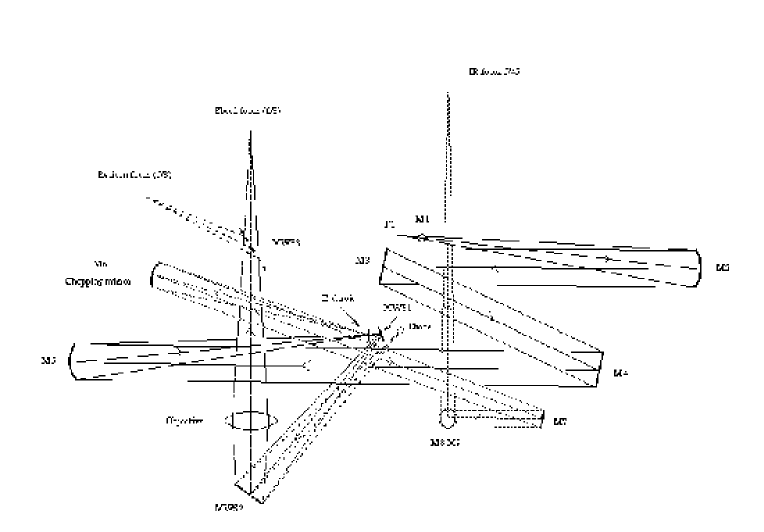
Figure 1: Optical layout of the ESO ADONIS adaptive optics system. The polarimeter, as a prefocal instrument, is installed at the entrance window of the dewar (IR focus f/45).

ADONIS is the ADaptive Optics Near INfrared System (see e.g. Beuzit & Hubin BH (1993) or Beuzit et al. beuzit (1997)) supported by ESO for common users since December 1994 at the F/8.1 Cassegrain focus of the La Silla 3.6 m telescope. Fig  1 shows the optical layout of the ADONIS adaptive optics (AO) system. A tip-tilt and a 64 element deformable mirror corrects the distortions of the image in real time and a Shack-Hartmann wavefront sensor (WFS) provides the difference signal for the deformable mirror using a bright reference star close to the object. The detector for the Shack Hartmann sensor can be chosen as either an intensified Reticon for bright sources (m_v $<$ 8 mag.) or an electron bombarded CCD for fainter sources (8 $<$ m_v $<$ 13 mag., 25 to 200Hz sampling). Both detectors are sensitive in the visible wavelength region. An off-axis tiltable mirror allows the sky background, in a field of radius $\leq$30^′′, to be chopped with the on-source image. The output F/45 focus delivers the image to a near-IR detector - either a Rockwell 256² HgCdTe array (SHARP II for 1-2.5$\mu$m, Hofmann et al. hofmann (1995)) or a LIR HgCdTe 128² anti-blooming CCD (COMIC for 1-5$\mu$m, Marco et al. marco (1996)).

2.2 The camera

The SHARP II camera was selected for the near-IR polarimetric observations. This camera has a fast shutter at the internal cold Lyot stop, allowing integration times as short as 20msec. The present observations were made with the standard J, H, K filter set and a narrow band 2.15$\mu$m continuum filter, with a width of 0.017$\mu$m, and denoted hereafter K_c.

2.3 The polarizer

The polarizer, from Graseby Inc., is a wire grid of 0.25$\mu$m period, on a CaF₂ subtrate. It is especially designed to work in the spectral range 1 to 9$\mu$m and has a transmission of 83% perpendicular to the wire grid at 1.5$\mu$m. It is remotely rotated by the ADOCAM control system to any desired absolute position angle within tolerances of 0.1^∘. This polarizer, as a pre-focal instrument, is inserted into the beam in front of the camera; and is not cooled. However since the polarizer is not oriented perfectly perpendicular to the optical axis there is a small image motion on the detector when rotating the polarizer (see Sect. 4.4 and Fig. 5).

3 Observational technique

The magnification giving a pixel scale of 0.05^′′ has been selected to ensure an adequate sampling of the PSF, at H band. The field was thus 12.8$\times$12.8^′′; for the study of extended sources larger than the field size it is obviously necessary to employ several pointings and mosaic the resulting images after basic data reduction. ADONIS has a limit of 30^′′ for the radial extent of the offset sky so values less than [30 - half detector size] (^′′) must be employed in order to have unvignetted sky background frames. Special care has been taken in the selection of the offset sky position to avoid any overlapping with the extended object observed. For all sources, object and chopped sky images were obtained at each position of the polarizer. A data cube of 256$\times$256 spatial pixels $\times$ M frames, where M is the number of object and sky frames, was acquired. Table 1 lists the details of the ADONIS polarimetry observations of the science and calibration sources.

Sets of chopped images were obtained at nine different positions of the polarizer, each 22.5^∘ apart, from 0 to 180^∘. The minimum number of frames required to determine the linear polarization and its position angle is 3 (spanning more than 90^∘ in position angle). By effectively oversampling the polarization curve (viz. the variation of detected signal with polarizer rotation angle) one can at least hope to average out shorter term variations in atmospheric transmission in order to improve the quality of the polarization measurement. Expressed in terms of the Stokes parameters I, Q and U (see e.g. Azzam & Bashara azzb (1987)), I depends on the total signal whilst Q and U depend on the difference in signals between images taken at polarizer angles of 0, 90, 45 and 135^∘. Then the linear polarization p is given by,    $p(\%)=100\times\sqrt{(}q^{2}+u^{2})$    where q=Q/I and u=U/I. The position angle of linear polarization is,    $\theta(^{\circ})=28.648\times tan^{-1}(U/Q)$    (Serkowski serk (1962)). Determining the polarization from $\geq$ twice as many images as necessary leads to improvement in polarization accuracy provided that any photometric variations are on timescales different from the exposure time of individual images at each polarizer angle. The worst case scenario is when photometric variations occur on a timescale similar to the exposure times, so that the measured difference signals vary wildy - the polarization determined by fitting a cosine curve then approaches zero. The chosen exposure times per polarizer angle were in the range 1 to 50 s depending on the source brightness (see Table 1). Observing a polarized source with the polarizer at 0 and 180^∘ polarizer positions should give the same detected counts and is therefore a direct way to monitor the photometric variations during the observational sequence. Column 8 of Table 1 lists half the difference (in percentage) between integrated counts in the star profile for the 0 and 180^∘ images (i.e. rms on the mean of the 0 and 180^∘ signal values). For R Monocerotis, the semi-stellar peak of the reflection nebula NGC 2261, the aperture covers the central extended source (full extent 8^′′), whilst for OH 0739-14, a reflection nebula around an embedded young star, an area 10^′′ in size was used for the statistics.

Source	Type	Date	Band	No.	Texp	No. Poln.	0-180∘
				Frms.	(ms)	sequence	semi-difference (%)
HD 93737	Low poln.	1996 Mar 02	K	20	50	3	0.76,0.65,0.22
	standard.	1996 Mar 03	H	20	50	2	2.32,1.01
		1996 Mar 04	J	20	40	1	0.15
HD 64299	Low poln.	1996 Mar 03	J	10	5000	1	0.11
	star		H	10	3000	1	1.01
			K	10	3000	1	0.89
		1996 Mar 04	J	3	10000	1	0.05
			H	3	6000	1	0.05
			K	5	10000	1	0.65
HD 94510	Low poln.	1996 Mar 04	Kc	30	40000	1	0.32
	star
OH 0739-41	Extended IR	1996 Mar 02	J	4	30000	1	0.45
	poln. source		H	4	5000	1	0.48
			K	4	5000	1	0.20
R Monocerotis	Extended IR	1996 Mar 03	J	10	1000	1	1.26
	poln. source		H	20	400	1	0.24
			K	30	100	1	0.18
$\eta$ Carinae	Polarized	1996 Mar 02	K	200	50	4
	source	1996 Mar 03	H	200	50	2
			H	100	50	1
		1996 Mar 04	J	200	50	2
			Kc	100	50	2

Table 1: List of polarization sources observed. The exposure time (T_exp) is given per frame.

4 Data reduction

The data reduction applied to AO polarimetry data consists of the removal of the detector signature and sky subtraction, which is common to IR imaging in general, followed by registration and derivation of the polarization parameters.

4.1 Removal of the detector signature

The basic data reduction steps were performed with the ‘eclipse’ package (Devillard nico (1997)). Flat-fields were acquired on the twilight sky at the beginning of each night of observation, in an exactly similar way as for the targets, at nine angles of the polarizer. The integration times were 7, 10 and 20s for the J, H and K bands respectively; no flat field was taken with the K_c filter. The flat field images must first be processed to flag bad pixels, caused by either permanently dead pixels or ones whose sensitivity undergoes large fluctuation during the exposure. Two methods have been employed depending on the number of frames available in a cube: sky variation or median threshold.

The ‘sky variation’ method works on a data cube, with preferably many planes (${}^{>}_{\sim}$20) in order to obtain reliable statistics on the variations. The standard deviation ($\sigma$) with frame number is computed for each pixel in the frame. A histogram plot of the standard deviations has a Gaussian shape representing the response to the, assumed constant, sky signal. All pixels whose response is too low (dead) or too high (noisy), compared to a central $\pm\sigma/2$ interval, are rejected. The ‘median threshold’ method can be applied to a small number of input frames (such as flat field data) and detects the presence of spikes above or below the local mean in each individual image independently. If the signal is assumed to be smooth enough, bad pixels are found by computing the difference between the image and its median filtered version, and thresholding it. This latter method is not as stringent as using the temporal variation, but is the only possibility when there are an insufficient number of images to calculate reliable statistics. Some bad pixels may however remain in the images after applying the bad pixel correction by either method; however the number is small and they can be manually added to the bad pixel map. Slightly different bad pixel maps were found for the different positions of the polarizer; which could be explained by a polarization sensitivity of the pixels ($\sim$1%), since the NICMOS detector sensitivity is slightly polarization dependent, or simply by the random variation of hot pixels.

Once corrected for the bad pixels, the twilight flats were normalized, then multiple exposures were averaged for the same position of the polarizer to derive the flat field maps. The target data cubes were corrected with the bad pixel map derived using the ‘sky variation’ method from the background sky frames and divided by the flat-field to give flat-fielded, cleaned images, where the sky contribution is still to be subtracted. All these operations were performed independently for the nine positions of the polarizer.

4.2 Sky subtraction

The sky background can be bright in the IR and may also be polarized so it is criticical in the case of polarimetry to ensure that the uncertainties introduced by sky subtraction are minimized. Several tests were performed to determine the impact of the method of sky subtraction, in conjunction with the bad pixel correction, on the data. The first method considers one sky and a bad pixel map for each position of the polarizer; the second method a single averaged sky (all polarizer positions confounded) but individual bad pixel maps for each position; whilst the third method uses the same averaged sky and bad pixel map for all polarizer angles.

All three methods were tested (Ageorges nancy (1997)) and the results demonstrated that the largest modification of pixel values, and therefore photometry, comes from the bad pixel map used. The third method produced the largest discrepancies from the expected $cos(2\theta)$ curve, where $\theta$ is the polarizer position angle. The first method is clearly to be preferred since the effect of any polarization of the sky signal on the target data is correctly removed and any short term variation in sky background is subtracted.

It was found, from sky background level in the polarization calibrator data, that the sky subtraction has been successful to better than 1% (rms noise of 3.5 ADUs). For the 0 and 180^∘ data, a further test of the quality of the sky subtraction was performed: the skies have been exchanged, i.e. ’sky 0’ has been used for the data taken at PA 180^∘ and conversely. This resulted in ’photometric’ variations less than 0.05%, thus giving us further confidence in our sky subtraction method.

4.3 Photometric quality

The photometric quality of the data can be checked in two different ways: either by comparing the photometry of an object when acquired at 0^∘ and at 180^∘ or by plotting the measured signal against the polarizer angle where a $cos(2\theta)$ form should be obtained for polarized data. The latter is illustrated in Fig. 2, for J band data of the NE lobe of the Homunculus nebula around $\eta$ Carinae. The signal is plotted with time as the polarizer was rotated from 0 to 180^∘; every ensemble of 200 points (within the dashed vertical lines) corresponds to frames acquired at the same position of the polarizer. The spread of points at a given polarizer angle gives a measure of the photometric variation.

The images, used to create this plot, have been overexposed on purpose in order to get as much signal as possible on the faint nebula. The central region of the images has thus been obtained outside the linear regime of the CCD. The intensity variation over this image has thus been recalculated avoiding a 30$\times$30 pixels area centered on $\eta$ Car. This is represented Fig. 2 together with a plot of the intensity variation over a 50$\times$ 50 pixels area centered on a lobe of the nebula, away from $\eta$ Car and thus obtained in the linear regime of the CCD. observed above is reduced by a factor of 2. Fig. 3, representing the photometric variation of frames acquired at 0 and 180^∘, clearly illustrates the fact that the night of these observations was not photometric: there is a 0.3mag. extinction of the data acquired at 0^∘ compared to that at 180^∘.

In Fig. 2 it is clear that there is a discrepant point, at 157.5^∘, since this does not fit into the smooth $cos(2\theta)$ progression of the curve. This problem, found for every source observed, was attributed to a technical problem of unknown origin; it appears from the figure that the polarizer may actually have been at an angle of 45^∘. All maps taken at this polarizer angle were ignored in the subsequent derivation of polarization parameters, thus reducing the number of independent polarizer angles to 7 (0 and 180^∘ being equivalent).

4.4 Derivation of polarization maps

The polarization degree for each pixel, binned pixel area or within an aperture was determined by fitting a $cos(2\theta)$ curve to the variation of signal with polarizer rotation angle $\theta$ for the eight signal values (excluding the value at 157.5^∘). A least-squares procedure was used with linearization of the fitting function and weighting by the inverse square of the errors (Bevington bev (1969)). The error on the polarization was determined from the inverted curvature matrix and the error on the position angle by the classical expression (Serkowski serk (1962)):    $\sigma_{\theta}(deg.)=28.648(\sigma_{p}/p)$    when $\sigma_{p}/p$ was $\geq$8 or from the error distribution of $\sigma_{\theta}/\theta$ given by Naghizadeh-Khouei & Clarke (nag (1993)) when $\sigma_{p}/p\leq 8$. The errors on the individual points in the images at each polarizer rotation angle take into account the number of images averaged, the read-out noise and the sky background contribution. Since the detector offset is not fixed per image it was necessary to bootstrap for the value of the sky level. A series of polarization maps were made with increasing sky contribution at a fixed polarization error per pixel. The sky signal was adopted when it produced polarization vectors which began to deviate from the expected centrosymmetric pattern (e.g. to the NE of R Mon - see Fig. 6) in the regions of lowest signal. Thus the polarization errors are not absolute errors. Applying a polarization error cut-off to the maps produces maps consistent with the expected structure (which can also be partially checked by binning the data). Fig. 4 shows a typical fit to the $cos(2\theta)$ curve for a 8$\times$8 pixels binned region of the R Monocerotis H band image (see Table 1 and Fig. 6). The error bars on the individual points arise from the photon statistics on the object and sky frames, with read-out noise considered.

It was noted in Sect. 2.3 that the rotation of the polarizer induces an image shift on the detector. Fig. 5 is an illustration of the displacement observed, for images of $\eta$ Carinae in K_c, while rotating the polarizer from 0^∘ to 180^∘ in steps of 22.5^∘ (see Sect. 3 for details on the observation procedure). Since the PSF is variable in time, reproducability is not guaranteed. However the displacements were found to agree with those in Fig. 5 for different targets (mostly unpolarized standard stars - see Table 1), and in different filters, to better than 0.5 pixel and so were adopted to register the images at different polarizer angles.

For a point source, where only the integrated polarization is of interest, the exact position of the source is not relevant provided all the signal is included in the summing aperture. However for extended sources, such as for $\eta$ Carinae and the Homunculus nebula, a polarization map which exploits the available spatial resolution is desired. It is therefore extremely important to ensure that the data are centered on the same position for all position angles observed, to avoid some smearing of the information. For unsaturated stellar images, the centroid of the point source can be used as a fiducial to shift the images to a common centre. In the case of saturated images it proved possible to obtain reliable centering by using a very large aperture for the centroid; this is then weighted by the outer (unsaturated) regions of the PSF. However if the source is polarized, and in particular if there is polarization structure across the point source then centroids at particular angles will be dependent on the source polarization. It was found that if the images were shifted to match the centroids at the 8 polarizer angles for the R Mon data, then a map with uniform, almost zero, polarization was derived, in contradiction to the known (aperture) polarimetry of this source (e.g. Minchin et al. minchin (1991)). In such a case the set of image shifts, derived from unpolarized point sources (Fig. 5), were applied to the data and the polarization maps were determined. Fig. 6 shows the resulting J, H and K polarization vector maps superposed on logarithmic intensity plots; the raw data has been binned 4$\times$4 pixels, i.e. 0.2^′′. Those shifts applied are closer to reality than those determined by the centroid of R Mon, but good to within $\pm$0.5 pixel. This might explain the difference in structure between our H band map and that of Close et al. (close (1997)). extract of the Close et al. map. Considerable structure across the central (almost point) source is evident. The cut-off of the maps is determined by the value of the 1$\sigma$ polarization error (4, 4 and 6% respectively for J, H and K). The structures seen in the J, H & K band maps (Fig. 6) change with wavelength, which might be an optical depth effect of the inclined disk. The striking difference between the maps in Fig. 6 and the one reproduced in Ageorges & Walsh (agewal (1997)) comes from the calibration of the data. Indeed the latter were preliminary results and the first polarization maps derived with ADONIS.

5 Calibration of the polarimetric data

In order to determine the source intrinsic polarization and its position angle, several corrections are necessary. The instrument possesses an instrumental polarization which must be vectorially subtracted from the measured polarization. The instrumental contribution is derived from the observation of unpolarized standards. The interstellar medium between the source and the observer also possesses an intrinsic polarization which needs to be corrected. The typical ISM polarization values are $\leq$2% and can be neglected when observing high polarization sources. If the ISM polarization is not negligible, then it must be determined from measurements of stars in the neighbourhood of the source (see e.g. Vrba et al. vrba (1976)); alternatively the distance dependence of the ISM polarization must be determined from measurements of many stars. The zero point of the polarization position angle is checked by observing non variable polarized standards, or polarized sources with reliable measurements. The lattest offer an excellent check on the polarizing efficiency of the instrument (i.e. response to a 100% polarized source should be 100%).

5.1 Sky polarization

In the optical during dark time the sky polarization is typically 3-4% (Scarrott, private communication). In the nights of our measurements, the sky polarization has been found to be consistent with zero within the error bars (typically $\leq$0.5%). Since it is the ratio of polarized intensity between the source and the sky that matters most and since the latter have carefully been subtracted (see Section 4.2), the sky contribution has been ignored in processing the data.

5.2 Instrumental calibration

5.2.1 Choice of the polarization calibrators

Despite extensive polarization observations, there is a distinct lack of any such standards in the IR. The polarized reflection nebulae OH 0739-41 and NGC 2261 (illuminated by R Monocerotis) were observed because of their extensive IR polarization data (Heckert & Zeilik heckert (1983) and Shure et al. shure (1995) for OH 0739-14, Minchin et al. minchin (1991) and Close et al. close (1997) for R Mon), although neither can be claimed as true, non-varying standards.

Since the observations are achieved using an adaptive optics system, the polarization standard could also be used as a PSF calibrator. Since the correction is optimized continuously, the resulting PSF is variable in time. Any point source observed as PSF calibrator needs to be close ($<$ 10^∘) to the target and be as similar as possible in terms of visible magnitude and spectral type, to ensure identical correction efficiency. Owing to the lack of polarization standards in the infrared, the polarization calibrators were chosen to be as close as possible to the source and bright enough to be used as reference for the wavefront sensor. In two cases, for HD 64299 and HD 95410, which have, respectively a B polarization of 0.151% (Turnshek et al. turnshek (1990)) and a V polarization of 0.004% (Tinbergen tinbergen (1979)) it was assumed that the IR polarization is negligible, although no measurements exist at these wavelengths.

In reducing the data taken on 1996 March 02 it was found that the derived polarization for any source (even OH 0739-14) was consistent with zero polarization, and, in addition, did not exhibit the expected shift of image centroid with polarizer angle (Fig. 5. Either the photometric conditions were exceptionally poor (this is not borne out by large discrepancies between the 0 and 180^∘ signal values - see Table 1) or, more probably, an instrumental problem, such as the polarizer not rotating to the requested angle, was present. The polarization information was therefore discarded for this night. However the K band image of $\eta$ Carinae had excellent spatial resolution and was retained (Walsh & Ageorges, walage (1999)).

5.2.2 ADONIS instrumental polarization

For the unpolarized (actually low polarization) standards, the integrated counts within a circular aperture including all the flux from the star profile (radius typically 2^′′) above the sky background was measured for each angle of the polarizer and a $cos(2\theta)$ curve fitted to the data. Table 2 lists the results. HD 93737 has a measured V band polarization of 1.07% at position angle 122.4^∘ (Mathewson & Ford matfor (1970)). Given the typical shape of the interstellar extinction curve (the ‘Serkowski law’, see e.g. Whittet whittet (1993)), the probable values of the interstellar polarization for this star, assumed to have a typical Galactic interstellar extinction, are 0.5, 0.3 and 0.2% at J, H and K respectively. The position angle is usually similar between the visible and IR (see eg. Whittet et al. whitgera (1994)). For the purposes of computing the instrumental polarization it was assumed that the polarization was zero. The first two sets of data on HD 93737 on 1996 Mar 02 (see Table 1) are not included on account of the problem with the data on that first night (see Sect. 5.2). In addition the first sequence of H band data on HD 93737 had poor photometry (see Table 1) and was not considered. There is a spread in the values indicating typical errors of $\pm$0.3% in linear polarization and $\pm$15^∘ in position angle. Given the errors the J, H and K values are consistent with an instrumental polarization of 1.7%. Adopted values are listed in the last row of the Table 2. Given that only a single measurement was performed at K_c, it is probably not significant that the instrumental polarization in this band is higher and that the position angle differs from the K band measurement.

Target	Date	J	H	K	Kc
		Linear poln. (%) & PA (∘)
HD 93737	1996 Mar 02			1.71,  88
	1996 Mar 03		1.59,  89
HD 64299	1996 Mar 03	1.51, 111	1.99,  86	2.16, 136
	1996 Mar 04	1.67,  97	1.48, 112	1.71,  89
HD 94510	1994 Mar 04	2.12, 104			2.05, 140
Mean	-	1.74, 105	1.69,  96	1.86, 104
Adopted	-	1.7,   105	1.7,    90	1.7,    90	2.0,   140

Table 2: Polarization of low polarization stars - instrumental polarization measurement

Once the instrumental polarization (intensity and angle) is determined this correction can be applied to the polarization maps point-by-point. Goodrich (goodrich (1986), in Appendix) describes the application of the instrumental correction.

5.2.3 Position angle calibration

On producing polarization maps for the Homunculus nebula around $\eta$ Carinae, it was noticed that the polarization vectors did not point back to the position of $\eta$ Carinae. There is no reason for such a behaviour since it is known to be a reflection nebula. If the illumination were by an extended source then the offset should not be one of simple rotation. A novel method was used to determine the single offset required to aligned all the polarization vectors in a centrosymmetric pattern around the position of $\eta$ Carinae. A least squares problem was solved to minimize the impact parameter at the position of $\eta$ Carinae produced by the perpendiculars to all the polarization vectors in the Homunculus by application of a single rotation. A consistent value of 18$\pm$1^∘ was found for the J, H and K images. In order to verify that this was not an artifact of the $\eta$ Carinae nebula and the fact that the central point source was saturated, the 18^∘ correction was applied to the polarization maps of NGC 2261. It was found that the vectors in the high polarization spur to the NE were well aligned with the direction expected for illumination by the peak of R Mon. Thus the calibration of the absolute position angle can be made without reference to a polarized standard.

Data source	Polarization (%) & PA (∘)
	J	H	K
This work (PA uncorrected)	10.6,  77	11.1,  74	8.1,  77
Minchin et al. minchin (1991)	11.1, 100	8.5, 103	5.6, 102

Table 3: JHK Polarization of R Monocerotis in an 8^′′ aperture

6 Results on restoration of polarization images

In order to measure polarization structure in the vicinity of a bright point source, it is necessary to deconvolve the point source response from the data frames taken at each position angle of the polarizer and then to form the polarization maps from the deconvolved images. The aim here is to detect polarization structure within an offset distance of a few times the diffraction limit from the point source. Several different approaches to restoration have been attempted in order to obtain detailed information on the fine structure of the Homunculus nebula close to the central source $\eta$ Carinae. This was motivated by the need to detect and measure the polarization of the three knots found in the 0.4^′′ vicinity of $\eta$ Car by speckle imaging in the optical (Weigelt & Ebersberger weiebe (1986) and Falcke et al. falcke (1996)). The polarization data for $\eta$ Car will be used to exemplify these experiments; the scientific conclusions will be reported in Walsh & Ageorges (walage (1999)). A preliminary discussion of restoration of these images, without considering the polarization, has been given by Ageorges & Walsh (agewalspie (1998)).

6.1 Image restoration trial

Two deconvolution techniques have been applied to the data: Richardson-Lucy (R-L) iterative deconvolution (Lucy lucy (1974), Richardson richard (1972)) and blind deconvolution (‘IDAC’, Jefferies & Christou jeff (1993), Christou et al. christou1 (1997)). The major difference between these methods is related to the treatment of the point spread function (PSF). With the Richardson-Lucy method, a PSF is required a priori to deconvolve the data, while for blind deconvolution, the PSF is determined from variations in the target object data. The blind deconvolution method uses an initial estimate, which can be a Gaussian for example. Since the adaptive optics PSF changes with time and is not spatially invariant (see e.g. Christou et al. christou2 (1998)) , blind deconvolution should be better suited than the Richardson-Lucy method, which assumes a PSF constant in time. The exact spatial variation of the AO PSF is not known. However in the present case, this is a minor problem since the source itself ($\eta$ Car) has been used as wavefront sensor reference star. Moreover with the pixel scale chosen, all the valuable information in the short band data is enclosed in the isoplanatic angle; the spatial variation of the PSF is thus negligible over the area of the $\eta$ Carinae images, which is not the case for the time variation.

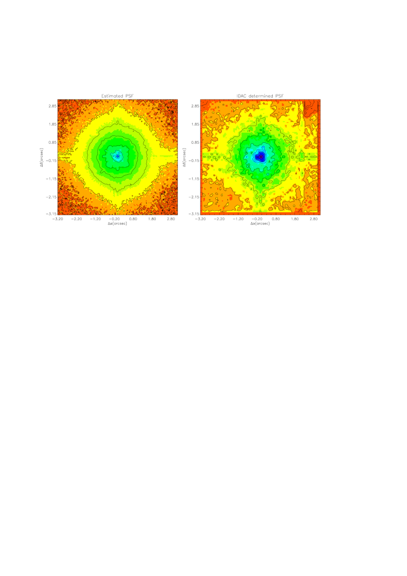
Figure 8: PSF estimated (left) and obtained (right) from an IDAC blind deconvolution of the K_c image of $\eta$ Car (see Table 2 for observational details). The PSF estimate is the shift-and-add of the point source (HD 94510) observed shortly before the target data with the K_c filter. It has been used as first guess for blind deconvolution.

A comparison of the Richardson-Lucy method and IDAC - ’Iterative Deconvolution Algorithm in C’, i.e the blind deconvolution algorithm used, was made using the K_c data on $\eta$ Car (Table 2). The aim was to test the reality of structures revealed in the near environment of the central star of this reflection nebula. For the R-L restoration, the Lucy-Hook algorithm (Hook & Lucy hook (1994)), in its software implementation under IRAF (‘plucy’), was employed. The principle is the same as for the Richardson-Lucy method, except that it restores in two channels, one for the point source and the other for the background (considered smooth at some spatial scale). The estimated position of the point source is provided and the initial guess for the background is flat. K_c data taken at polarizer angles of 0 and 180^∘ were restored (called K_c0 and K_c180). For the K_c0 image, blind deconvolution was also performed. It should be noted that although the polarizer angles are effectively identical, the Strehl ratio is not identical between the two data sets (K${}_{c}^{1}$ & K${}_{c}^{2}$) and is higher for K${}_{c}^{1}$ (27.9% against 22.1%). Although this could be considered an advantage, it has a drawback since the four bumps around the PSF (see Fig. 8 for the appearance of the PSF) are more pronounced. These bumps (‘waffle pattern’) correspond to a null mode of the wavefront sensor as a result of an inadequacy in the control loop. The problem of the four bumps distributed symetrically around the source is that although they are in the PSF they do not vary; they are fixed in time and position and therefore not removed from the image as part of the PSF. There is however a way to overcome this problem, and that is by forcing them to be in the PSF.

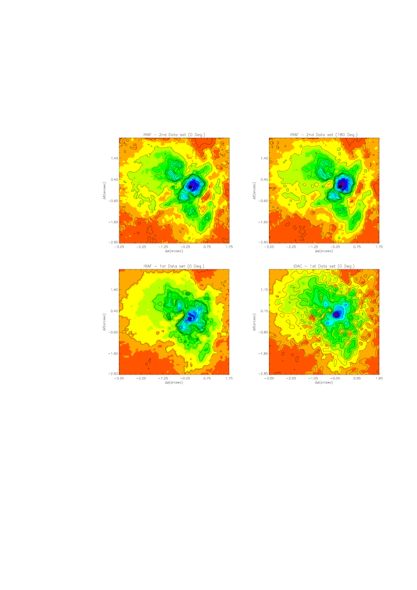
Figure 7: Comparison of the results of two deconvolution techniques for K_c data of $\eta$ Carinae and the Homunculus nebula. On the top row are shown data from the second polarizer sequence, at 0 (left) and 180^∘ (right), both deconvolved with ‘plucy’ and convolved with a Gaussian of 3 pixels FWHM. The bottom left image is identical to the top left one but the data restored is from the first polarizer sequence (0^∘ image). The result of blind deconvolution is presented in the bottom right hand image for the first data set - K${}_{c}^{1}$ - at 0^∘ polarizer angle.

Fig. 7 presents the deconvolution results obtained with both methods on the two separate data sets (Table 1) and Fig. 8 shows the PSF derived from blind deconvolution. The ’plucy’ deconvolved data have been restored to convergence and then convolved with a Gaussian of 3 pixels FWHM. The blind deconvolved data were not restored to convergence but limited to 1000 iterations to be comparable, in terms of number of iterations, with the Lucy deconvolution. The resulting image seems thus more noisy than the Lucy deconvolved ones. Note that neither of the methods used succeeded in removing the 4 bumps from the K_c images of the first observational sequence (K${}_{c}^{1}$0).

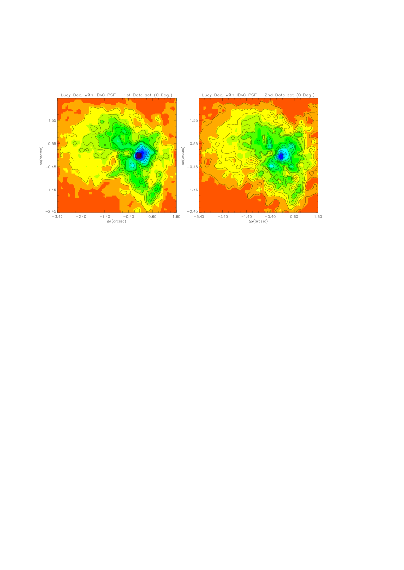
Figure 9: K_c data of $\eta$ Car. at 0^∘ for the two different data sets acquired. These images have been obtained after convergence of the blind deconvolution algorithm and reconvolution with a Gaussian of 3 pixels FWHM. This has to be compared with the right hand pictures of figure  7 top and bottom respectively, which are the equivalent results for ‘plucy‘ deconvolution.

The data acquired at the polarizer position angles of 0 and 180^∘, deconvolved with the same algorithm (‘plucy’) both show identical structures (upper row of Fig. 7). This example serves to illustrate the stability of the ‘plucy’ method when applied to AO data while using a reasonable PSF estimate. The image from the first polarizer sequence, polarizer angle 0^∘, deconvolved using IDAC is shown as the lower right image in Fig. 7 and is to be compared with the upper left image deconvolved with ‘plucy’. It is clear that similar structures appear in both restorations and that there are no significant features in one restoration which do not appear in the other. The differences in the images are mainly due to the fact that the blind deconvolution has been stopped before fully resolving the data and the final image is thus more noisy. Moreover the presence of the four bumps is enhanced in this image. The major difficulty in this deconvolution is that these noise structures are convolved with extended emission from the Homunculus nebula. Being in the middle of the nebula, the flux identified on these bumps is then a convolved product of the waffle pattern and the extended structure of the nebula. It is thus very difficult for the program to isolate these four ’point sources’ and recover properly the true shape of the nebula at these positions. In order to fully compare the different deconvolution techniques, blind deconvolution has been pushed to convergence for K_c0 (data set 1 & 2). The results (Fig. 9) are to be compared with the right hand side of Fig. 7. The structures close to $\eta$ Car emphasized by the two deconvolution processes, excluding the four bumps, confer a degree of confidence in the scientific results which will be presented in Walsh & Ageorges (walage (1999)).

6.2 Polarimetry restoration trial

In the case of polarimetric data, the deconvolution problem is more severe since the photometry must be preserved in the restored images in order to derive a polarization map. The Richardson-Lucy algorithm is superior to blind deconvolution in that it should preserve flux. Experiments were performed on the K_c $\eta$ Car data set, restoring each of the nine polarizer images with the PSF derived from the unpolarized standard at the same polarizer angle. The results were poor even when the restored image was convolved with a Gaussian of 3 pixels FWHM. They illustrate the effect of the variable PSF and thus the difficulty to recover polarization data at high angular resolution so close to the star. Huge fluctuations in the value of the polarization were seen in the vicinity of $\eta$ Car. The differing PSF of the unpolarized star and of $\eta$ Car (the AO correction was much better for the $\eta$ Car images than for the standard star) produced restored images with large differences in flux at a given pixel in the different polarization images. At present there is no known method to recover the true PSF from the data and conserve the flux through restoration. A possible (although computer intensive) solution is to determine the PSF from blind deconvolution and use the result for the PSF in another algorithm known to preserve the flux. This has been performed here: the PSF determined by blind deconvolution has been used both with the Richardson-Lucy and Lucy-Hook algorithms. Since the IDAC blind deconvolution algorithm normalised the input image at the beginning of the iterations, the final image was rescaled back to the original total count to allow error estimation of the polarization image. Polarization maps for the three methods (‘IDAC’ alone and combined with R-L and ‘plucy’ methods) have been created and compared after reconvolution with a 3 pixel Gaussian.

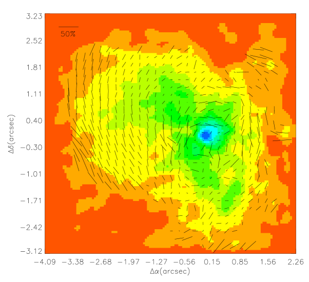
Figure 10: Polarization map of K_c deconvolved data of $\eta$ Car. overplotted on the high resolution intensity map. For clarity, the polarization vectors have been calculated on pixels binned 4 by 4 (0.2$\times$0.2^′′). The intensity map is at the nominal resolution of 0.1”

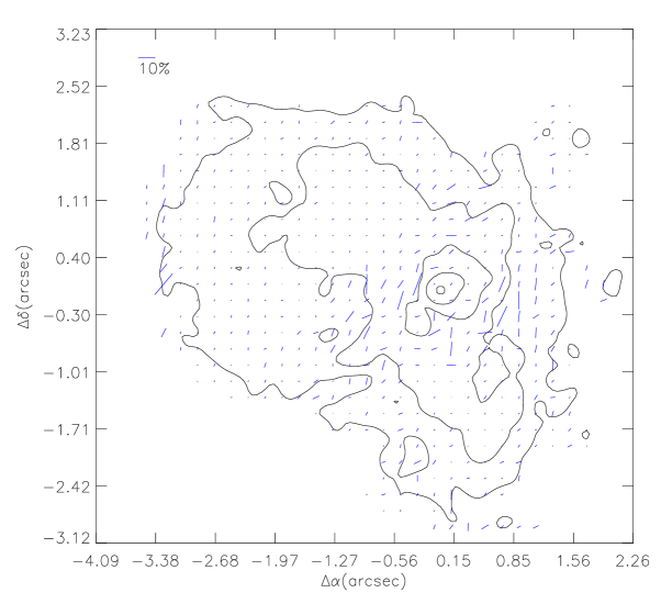
Figure 11: Differential polarization map of K_c deconvolved data of $\eta$ Carinae. It represents the difference between the polarization map derived after pure blind deconvolution and R-L deconvolution using the PSF derived by blind deconvolution. The errors are clearly under 5% except at the border and thus low signal$\_$to$\_$noise level of the nebula and at the position of the telescope spider ($\Delta\alpha$ and $\Delta\delta$ = 0). Compared to the rest of the map some bigger differences can also be found at $\approx$ 0.5” from $\eta$ Car and is attributed to the effect of the PSF wings in the deconvolution process.

From the high resolution restored images an attempt has been made to derive the polarization map. Fig. 10 illustrates the result obtained while using the PSF determined by the blind deconvolution with the R-L algorithm (30 iterations with the accelerated version), after reconvolution with a Gaussian of 3 pixel FWHM. The overall centro-symmetric pattern of polarization observed at larger scale and resolution is recognisable here as well. The major deviation from this pattern at $\Delta\alpha$ and $\Delta\delta$ zero (i.e. east-west and north-south through the image of $\eta$ Car) is due to the spider of the telescope. The presence of this feature is hard to identify on the intensity map underplotted but clearly present at this position in the original (undeconvolved) data. Fig. 11 is a vectorial difference between results obtained with Lucy deconvolution and blind deconvolution. Special care has been taken to avoid the vector difference to add when the position angles were separated by close to 2$\pi$. Some vectors at the border of the noise cut-off (e.g. at $\Delta\alpha\approx-3.0^{\prime\prime}$) detected in the Lucy map but not in the other are not represented here to avoid confusion with the differential vectors plotted. Major differences can be found at approximately 0.5^′′ from the center and correspond to differences in the deconvolution due to the wings of $\eta$ Carinae. At $\Delta\alpha$ = 0 and $\Delta\delta$ = 0 $\pm$ 0.3^′′, the important difference between the two reconstructed polarization maps is meaningless since these positions correspond to the spider of the telescope and the data are poorly restored here.

7 Conclusions

The process of data acquisition and reduction for polarization observations taken with the ESO ADONIS adaptive optics system has been described. Whilst certain precautions both in the observing method and in data reduction are required for imaging polarimetry and adaptive optics seperately, several other problems are presented arising from the combination of the two methods.

• Since the PSF varies in time the wavefront sensor reference star should be as similar as possible to the target object in terms of brightness (since the achieved Strehl ratio strongly depends on the reference star magnitude) and spectral characteristic, to ensure similar AO correction. Since the PSF varies across the field of view (depending on the anisoplanatic angle), it is also preferable to select the WFS reference star as close as possible to the target object. In practice this is rarely achieved when the target itself can not be used as WFS reference star. However a good estimate of the PSF provided by the reference star allows accurate deconvolution of the target without the introduction of artifacts arising from the differing PSF’s.

• Imaging polarimetry requires good photometric conditions. By oversampling the cos(2$\theta$) polarization curve at more than three position angles of the polarization analyser, an averaging over the photometric conditions is achieved. However depending on the time period of the photometric variations the averaging can result in zero polarization even from a substantially polarized source. In principle the use of an AO system should not compromise the photometric quality of the observations.

• The two polarization calibrations that are required impose the observation of an unpolarized source, to determine the instrumental polarization, and of a target with known polarization, to calibrate the angle of polarization. In the IR there is a very distinct lack of unpolarized and polarized standards. Stars with known very low optical polarization are suitable as IR unpolarized standards since the Serkowski interstellar polarization law shows that the polarization is much less in the IR than the optical. However polarized standards typically have a circumstellar origin to their high polarization and the value in the IR cannot be predicted. Many of the reflection nebulae around Young Stellar Objects have variable polarization and are therefore not ideal polarized standards.

Several strategies have been described for flat fielding and sky subtraction and it was shown how deviations from the expected cos(2$\theta$) curve can give an indication of the photometric conditions at the time of observation and allow any discrepant polarizer angles to be discarded as was found for the ADONIS polarizer at PA 157.5^∘. The instrumental polarization for ADONIS was determined at 1.7% over the J, H and K range. Polarization maps have been succesfully produced for the reflection nebula around $\eta$ Carinae (the Homunculus). By using the PSF’s determined from blind deconvolution at the same polarizer angles as the data, it has been shown that polarization structure can be revealed as close as two times the diffraction limit to a point source. The interpretation of the ADONIS AO polarization results on $\eta$ Carinae will be presented in a forthcoming paper (Walsh & Ageorges walage (1999)).

8 Acknowledgements

We would like to thank the ESO ADONIS team for their advice and help during the development of the data reduction strategy. S. M. Scarrott is also acknowledged for useful comments on imaging polarimetry.

Figure 2: The photometric variation of the basic data is illustrated by the time sequence of measured counts in a region of the Homunculus taken in J band. Every 200 frames, the polarizer has been rotated by 22.5^∘ and the vertical dashed lines indicate the change of polarizer position angle. The width of this curve is characteristic of the photometric variations. The discrepant point at 157.5^∘ is attributable to an instrumental problem (see text). Left: global intensity variation over the full data frame but excluding a 30$\times$30 pixel box centered on $\eta$ Carinae; right: variation over a 50 $\times$ 50 pixel area of the nebula, far from the saturated center of the image.

Figure 3: Photometric variation between data taken at PA 0 and 180^∘ is shown for the full frame (excluding the central source, i.e. $\eta$ Car itself) at left, and for a small area centered on the Homunculus (right).

Figure 4: A typical fit of the observed signal as a function of polarizer rotator angle by $pcos(2\theta)$ for the summed counts in an aperture over the H band image of R Monocerotis (see Table 1 and Figure 6). The derived value of linear polarization and position angle is shown by the bold line. The point at 157.5^∘ was not considered in the fit.

Figure 5: Illustration of the variation of the position of the centroid of an image on the detector while rotating the polarizer from 0 to 180^∘ in steps of 22.5^∘. The target was $\eta$ Car observed in K_c band and the shifts are clockwise with increasing rotator angle.

Figure 6: J, H and K polarization maps of R Monocerotis and the brightest regions of the reflection nebulae NGC 2261. The contour maps shows the logarithm of the signal (polarized + unpolarized). The size of the polarization vectors is indicated and the orientation is north to the top and east left.

References

- (1) Ageorges N., 1997, ’Polarimetric measurements and Deconvolution Techniques’, Proceedings of the NATO-ASI summer school on “Laser guide star adaptive optics for Astronomy”, Cargèse 29 Sept. - 10 Oct. 1997
- (2) Ageorges N. & Walsh J.R., 1997, The Messenger 87, 39
- (3) Ageorges, N., Walsh, J. R., 1998, SPIE Proc. 3353, in press
- (4) Azzam R. M. A., Bashara, N. M.,1987, Ellipsometry and polarized light, Elsevier Science, Amsterdam
- (5) Bailey, J. A., Hough, J. H., 1982, PASP, 94, 618
- (6) Beichman C.A., Ridgway S., 1991, Physics Today, 44, 48
- (7) Berger J.-P., Ménard F., 1997, Poster proceedings of IAU Symposium 182 on Herbig-Haro objects and the birth of low mass stars, F. Malbet & A. Castet eds., 201
- (8) Bevington, P. R., 1969, Data Reduction and Error Analysis for the Physical Sciences, New York, McGraw-Hill
- (9) Beuzit J.-L. & Hubin N., 1993, The Messenger 71, 52
- (10) Beuzit et al., 1997, Experimental Astronomy 7, 285
- (11) Christou J. C., Bonaccini D., Ageorges N., 1997, Proc. of SPIE Vol. 3126, 68
- (12) Christou J.C., Marchis F., Ageorges N., Bonaccini D. & Rigaut F., 1998, SPIE Proc. 3353, in press
- (13) Close L. M. et al., 1997, ApJ 489, 210
- (14) Code A.D., Whitney B.A., 1995, ApJ 441, 400
- (15) Davis L. Jr., Greenstein J.L., 1951, ApJ 114, 206
- (16) Devillard N., 1997, The Messenger 87, 19
- (17) Draine, B. T., Lee, H. M., 1984, ApJ, 285, 89
- (18) Falcke, H., Davidson, K., Hofmann, K.-H., Weigelt, G., 1996, A&A, 306, L17
- (19) Fischer O., Henning Th., Yorke H.W., 1994, AA 284, 187
- (20) Goodrich, R. W., 1986, ApJ 311, 882
- (21) Heckert, P. A., Zeilik, M., 1983, MNRAS, 202, 531
- (22) Hodapp K.W., 1984, AA 141, 255
- (23) Hofmann R., Brandl B., Eckart A., Eisenhauer F., Tacconi-Garman L., 1995, Proc. SPIE 2475, 192
- (24) Hook R.N., Lucy L.B., 1994, Image restorations of high photometric quality. II. Examples. In Hanisch R.J. & White R.L. (eds) Space Telescope Science Institute, The restoration of HST images and spectra II, 86
- (25) Jefferies S.M., Christou J.C., 1993, ApJ 415, 862
- (26) Jones T.J., 1997, AJ 114, 1393
- (27) Lloyd-Hart M. et al., 1998, ApJ 493, 950
- (28) Lucy L., 1974, AJ 79, 745
- (29) Marco, O., Lacombe, F., Bonaccini, D., 1996, ESO Messenger, No. 85, 39
- (30) Mathewson, D. S., Ford, V. L., 1970, Mem. RAS, 74, 139
- (31) Mathis, J. S., 1990, ARAA, 28, 37
- (32) Minchin N. R. et al., 1991, MNRAS, 249, 707
- (33) Naghizadeh-Khouei, J., Clarke, D., 1993, A&A, 274, 968
- (34) Piirola V., Scaltriti F., Coyne G.V., 1992, Nature Vol 359, No. 6394, 399
- (35) Richardson W.H., 1972, J. Opt. Soc. Am. 62, 55
- (36) Rigaut F. et al., 1998, PASP 110, 152
- (37) Sahai R. et al., 1997, ApJ 492, L163
- (38) Serkowski, K., 1962, Adv. in A&A, ed. Z. Kopal, 1, 289
- (39) Sitko M.L. & Yudong Z., 1991, ApJ 369, 106
- (40) Shure, M., Sellgren K., Jones, T. J., Klebe, D., 1995, AJ, 109, 721
- (41) Tinbergen, J., 1979, A&ASS, 35, 325
- (42) Turnshek D.A. et al., 1990, AJ, 99, 1243
- (43) Vrba F.J., Strom S.E., Strom K.M., 1976, AJ 81, 958
- (44) Walsh, J. R., Ageorges, N., 1999, A&A, in preparation
- (45) Warren-Smith, R. F., 1983, MNRAS, 205, 337
- (46) Weigelt, G., Ebersberger, J., 1986, A&A, 163, L5
- (47) White, R. L., Schiffer, F. H., Mathis, J. S., 1980, ApJ, 241, 208
- (48) Whitney B.A., Hartmann L., 1992, ApJ 395, 529
- (49) Whittet, D. C. B., 1993, Dust in the Galactic Environment, Bristol, Inst. of Phys.
- (50) Whittet, D. C. B. et al., 1994, MNRAS 268, 1
- (51) Witt, A. N., 1977, ApJS, 35, 1