Globular Cluster Systems I: $V-I$ Color Distributions

Abstract

We have compiled data for the globular cluster systems of 50 galaxies from the HST WFPC2 archive, of which 43 are type S0 or earlier. In this paper, we present the data set and derive the $V-I$ color distributions. We derive the first four moments of the color distributions, as well as a measure for their non–unimodality. The number of globular clusters in each galaxy ranges from 18 (in NGC 2778) to 781 (NGC 5846). For those systems having more than 100 clusters, seven of sixteen (44%) show significant bimodality. Overall, roughly half of all the systems in our sample show hints of a bimodal color distribution. In general, the distributions of the faint galaxies are consistent with unimodality, whereas those of the brighter galaxies are not. We also find a number of systems with narrow color distributions—with both mean red and blue colors—suggesting that systems exist with only metal–rich or only metal–poor globular clusters. We discuss their possible origins.

In comparing the moments of the $V-I$ distributions with various galaxy properties for the early-type galaxies, we find the following difference in the correlations between the field and cluster galaxy populations: the peak $V-I$ color of the globular cluster distribution correlates well with the central velocity dispersion—and hence the Mg2 index and total luminosity—for galaxies in cluster environments; there exists no such correlation for field galaxies. This difference between cluster and field galaxies possibly reflects different formation scenarios for their globular cluster systems. Among the explanations for such a correlation, we consider either a larger age spread in the field populations or the possibility that cluster galaxies are always affected by significant accretion whereas some field galaxies could host pure “in situ” formed populations.

1 Introduction

In the past decade, globular cluster systems were established as powerful probes for the formation and evolution of galaxies (e.g. Harris 1991 and Ashman & Zepf 1998 for reviews). With very few exceptions, globular clusters exist in large numbers around all galaxies. They are not only easy to detect; their properties are readily influenced by the formation and evolution of their host galaxies and, in a larger sense, their environment. Globular cluster formation is also closely related to the star–formation history of the galaxies (e.g. Kissler-Patig et al. 1998a). The study of globular cluster systems, combined with the predictions of their properties from various galaxy formation scenarios, can therefore be used to constrain galaxy formation and evolution.

In recent years, tens of galaxies have been studied for their globular cluster population (e.g. compilation in Ashman & Zepf 1998). However, no systematic study of the properties of globular cluster systems, including more than a dozen hosts, has been carried out. Motivated by the need for a homogeneous study of a large number of systems, we have exploited the Archive of the Hubble Space Telescope as an ideal starting point for such a study, since it includes a large number of images centered on galaxies in different filters and taken in nearly identical conditions, leading to homogeneous photometry.

We begin by studying the properties of globular cluster systems around a large number of early–type galaxies, then describe the resulting sample in Sect. 2 and the pipeline reduction in Sect. 3. We study the color distributions of the systems (presented in Sect. 4 and 5), followed by a discussion of the properties of the color distributions, correlations among these properties, and their relation to the properties of the host galaxies (Sect. 6 and 7). Because color denotes a mix of age and metallicity of the systems, globular cluster systems have gained considerable interest after the discovery of multi–modal distributions in some systems (Zepf & Ashman 1993). Such a system implies that at least in some galaxies, globular clusters formed from several different mechanisms and possibly at several epochs. Color distributions alone are thus already a strong diagnostic for the history of the globular clusters systems and, by implication, for the history of the host galaxies. We discuss the properties of the color distributions of our sample for various formation scenarios in Sect. 8. In a companion paper, we use these data to constrain the models of Côté et al. (1998).

2 The Galaxy Sample

We searched the HST archive for all early-type galaxies that have been observed in two colors with adequate exposure times, using only WFPC2 data from a variety of programs, with the Nuker Group (PI: Faber and Richstone) providing most of it. 90% of the galaxies where observed in F555W ($V$) and F814W ($I$); some galaxies were observed through the F547M and the F450W filters which we transformed to $V$ (see below). We did not use data taken in other filters. Although we may have some some early-type galaxies, we attempted to make a complete study from the archive. Furthermore, some of the galaxies below are not early-types; we include them only for comparison, not for use in the analysis.

Table 1 presents the data properties for each galaxy: galaxy name (Col. 1), filter (Col. 2), total exposure time (Col. 3), number of individual exposures (Col. 4), and PI name and number (Col. 5). Three galaxies have more than one pointings and we include their total exposure times from all pointings. There are 50 galaxies in total. Table 2 summarizes the physical properties for the 43 galaxies which are S0 or earlier.

3 The Pipelined Reduction

We reduced all of the data starting from the individual exposure. The CADC provided the recalibrated science exposure (see cadcwww.dao.nrc.ca for details of the recalibration). All data were sent through a pipelined reduction. We divide the reduction into two steps: the combination of the individual images, and the photometry for the globular clusters. The first step requires shifting the images, scaling by exposure times, and combining. We use the HST header parameters for the telescope pointing (CRVAL1 and CRVAL2) to determine the shift. Instead of using the telescope pointing, we could have used reference objects in the images to measure the shift; for a handful of galaxies, we confirmed that the telescope pointing provides the same shift as when we used reference objects. We use a linear shift so as not to smear cosmic-ray affected pixels, then scale the images to a common exposure time. Different gains were used between galaxies and even among different exposures of the same galaxy. Finally, we transformed all images to gain 7. The combining process must be robust, as many of the galaxies have a limited number of individual exposures that make it difficult to remove cosmic-rays adequately. We therefore use a biweight estimate for the combining. The biweight attempts to estimate the mode of a distribution by using an iterative approach whereby deviant points are subsequently de-weighted. The parameters for the weighting result from numerical simulations (see Beers et al. 1991 and reference therein for a fuller explanation). Unfortunately, some galaxies only have two exposures in a given filter. To help decide whether a given pixel is an outlier, we include both filters in the combining process. We exclude the flagged pixels when combining in a given filter.

The second part of the reduction includes the photometry. Most of these data have the center of the galaxy in one of the WFPC2 chips (most are in the PC). To measure with greater reliability those clusters which have the high-background galaxy under them, we first subtract the galaxy light using a “median-filtering” technique; instead of the median, we use a biweight estimate (explained above) for the local flux value. We choose the parameters for the filtering—i.e., the inner radius equals 8 pixels and the outer radius equals 14 pixels—based on results from experiments with no background present. In addition, we make an initial pass to detect the globular clusters, then flag those pixels under the clusters to make sure the filtering technique does not include them when determining the galaxy component. We subtract the galaxy only in the chip that contains the galaxy center.

We use SExtractor (Bertin & Arnouts 1996) for the photometry, setting the finding parameters to 2 connected pixels 2.5 $\sigma$ over the local background as defined in a 32$\times$32 pixels box. The frames were further convolved with the PSF kernel given in the WFPC2 handbook for the respective chips in order to optimize the finding (see SExtractor manual, Bertin & Arnouts 1996).

We must correct the resulting magnitudes since the photometry is measured in a 2 pixel radius aperture. We correct the resulting magnitudes to a 0.5″ radius aperture, using the values proposed in Whitmore et al. (1997), and by 0.1 magnitude in order to extrapolate to the total light (see Holtzman et al. 1995). Finally, the magnitudes measured in the HST filter set were converted into the Johnson–Cousins $V$ and $I$ system by applying the transformations given in Holtzman et al. (1995). For the F555W and F814W filters used in the vast majority of our data sets, empirical transformations exists. For the F547M filter, we used the theoretical transformation into the $V$ filter. Finally, we used the empirical transformation to convert the F450W filter, used for the Fornax galaxies, into a Johnson $B$ filter, followed by a linear transformation from $B-I$ into $V-I$ derived from the populations synthesis models of Bruzual & Charlot (1993) for ages $>$ 5 Gyrs and the full range of available metallicities. The linear transformation follows $V-I=0.466~{}(B-I)+0.14$. The average uncertainty on the magnitudes is 0.06; this uncertainty scales with magnitude roughly so that at $V$=24 we have an uncertainty of 0.1, and at $V$=20 an uncertainty of 0.01. We go down to around 25.5 in $V$ and 24.5 in $I$, but we are only able to approximate both our limiting magnitude and uncertainty, given that the galaxies have a range of exposure times.

We note that the extrapolations from 2 pixel apertures to total magnitudes, derived for point sources, are extremely uncertain when applied to slightly extended objects such as globular clusters and can significantly affect the final magnitudes (see Kundu & Whitmore 1998, Puzia et al. 1999). However, the error of the extrapolation is similar in the F555W and F814W filters, so that the final colors are not affected by systematic errors of less than 0.03 magnitudes.

Finally, the data were corrected for foreground reddening using the maps of Schlegel et al. (1998), and the law E$(V-I)=1.55\cdot(B-V)$.

4 The $V-I$ color distribution of the systems

SExtractor provides an estimate of the magnitude, magnitude error, ellipticity, FWHM, and star/galaxy classification. From these measurements we select globular clusters from the objects that have the following criteria: a magnitude error smaller than 0.1; $V-I$ color between 0 and 2; ellipticity smaller than 0.5; FWHM between 1 and 4 pixels (on both the PC and WF chips); and ‘non-star’ classification (set to reject remaining cosmic rays and hot pixels, rather than to try to exclude point sources). No cut on the magnitude exists since it correlates with the magnitude error. The number of true globular clusters excluded by these criteria is typically less than 10%, somewhat higher for the most distant galaxies and those with short exposure times. The contamination by foreground stars and background galaxies passing our selection criteria is roughly constant and estimated from the Hubble Deep Field North (Williams et al.1996). The percentage of contamination depends on the distance and the richness of the globular cluster system considered, and lies around 5% for a typical system with $>100$ clusters at a distance of 10 to 20 Mpc. It can rise up to 30% to 50% for systems at significantly larger distances—that we then excluded in the following analysis where mentioned—or for systems with significantly less clusters.

Fig. 1 plots $V-I$ histograms for all of the 50 galaxies in the sample. As a histogram is the crudest form of density estimation, we also include the adaptive kernel density estimate as the solid line. A histogram is a density estimate that utilizes both discreet and equal-sized windows; it is therefore dependent on both the choice of the window size and the location of the window edges. More robust techniques include both weights for an individual datapoint’s contribution to a density estimate, and varying size that preserves the noise properties (i.e., sparse regions require larger binning). The adaptive kernel estimate contains these properties, provides a non-parametric density estimate on a grid. We refer to Silverman (1986) for a complete discussion of the adaptive kernel estimate. It works as follows: we obtain an initial density estimate, then adjust the window width at each grid element according to the initial density in such a way that low density regions have a large window width. We use the Epanechnikov kernel, an inverted parabola, for the density estimate. The result of an adaptive kernel estimate can be highly dependent on the initial smoothing, especially for small samples like ours with $N<100$; thus, we use least-squares cross-validation to choose the initial smoothing (see Silverman 1986, p. 48). This technique minimizes an estimate of the integrated square error given by $\int(\tilde{f}-f)^{2}$, where $\tilde{f}$ is the density estimated from the data—dependent on the window width (the smoothing parameter)—and $f$ is the underlying function we are trying to estimate. One point is removed from the sample, and we estimate the density for a given smoothing from the $N-1$ data points. Repeating this $N$ times and using the average provides an estimate of the underlying function $f$. The optimal smoothing is then the one that minimizes the estimated integrated square error.

The dotted lines in Fig. 1 represent the 90% confidence bands obtained through a bootstrap estimate, a technique that draws with replacement from the original sample of $N$ points. One bootstrap realization contains $N$ points, which are not necessarily unique. For each realization we estimate the distribution function and repeat this procedure 1000 times. At each grid element we then have a distribution of points, from which we choose the 5% and the 95% values, representing the 90% confidence band. These confidence bands reflect only the variance, not the bias, of the estimate. The bootstrap procedure includes the measurement uncertainties implicitly because they are reflected in the original estimate of the colors.

4.1 Measuring the Moments of the Distributions

Moments represent a simple quantification of the distributions to with which we correlate other galaxy properties (discussed below). However, due to small number statistics and contamination, we desire a more robust estimate for the moments other than the classical estimates. We therefore use the biweight estimate of location (1st moment) and scale (2nd moment), Finch’s asymmetry index (3rd moment), and the Tail Index (4th moment). Beers et al. (1991) describe the biweight estimators in detail. The asymmetry index measures skewness by comparing gaps between the ordered data points on both the right and left side of the distribution. The gaps are weighted according to their rank order, thereby devaluing the contribution from outliers. The Tail Index measures the spread of the dataset at the 90% level relative to the spread at 75%, and is normalized such that a Gaussian has an index equal one. Bird & Beers (1993) provide an explanation of the asymmetry index and tail index, and show that they are superior estimates compared to the classical skewness and kurtosis. Table 3 presents these robust moments and their 68% confidence band. A bootstrap procedure, the same as described above, provides the confidence bands. The galaxies listed in italics in Table 3 are late-type.

5 Relations between Moments and Galaxy Properties

In the following sections, we investigate the relations among the properties of the globular cluster color distributions and their relation to the properties of the host galaxies. We restrict ourselves to a homogeneous sample of globular cluster systems with best determined properties. We include S0’s and ellipticals, but exclude the late–type galaxies listed in italics in Table 3. We further restrict the sample to galaxies with redshift less than 3000 km s^-1 (excluding NGC 1700 and NGC 4881), since at anything smaller than this distance contaminating fore-/background objects present no problem. We set a lower limit of the number of globular clusters of 50, for which the moments are well defined. Finally, we exclude the systems that were not observed in the F555W and F814W filters to avoid systematic effects in the conversion to a homogeneous photometric system (excluding NGC 4374, NGC 1399, NGC 1404).

The restricted sample includes 26 globular cluster systems for which the distributions of properties are shown in Figure 2. Figure 2 presents all properties plotted against each other, as we discuss below. Examining the range of the $V-I$ moments shows a relatively sharp cut–off in the peak color at $V-I\simeq 1.12$. The width or scale appears to be around 0.16 for most systems, including an artificial broadening by photometric errors of around 0.06 typically, with only few systems having significantly broader distributions. Most of the systems are slightly positively skewed—i.e., they have the tendency to cut–off more sharply in the blue and extend somewhat towards the red. Finally, the tail index implies that most of the distributions have tail weight consistent with a Gaussian distribution.

5.1 Peak to the 2nd, 3rd, and 4th Moments

We show the relation between the peak and the scale (width) of the distributions in the first plot on the upper line in Figure 2; an enlarged version appears in Figure 3. We first notice that a blue cut-off is seen in all distributions, implying a lower metallicity limit for all globular clusters. This limitation imposes a lower cut–off in color and forbids a broadening of any distribution towards the extreme blue (about $V-I<0.8$). Therefore, in order to have a blue mean color, systems both must lack those red globular clusters that could not be compensated by extreme blue clusters and must be narrow. Interestingly, such systems with very little red clusters are observed in our sample, i.e. seem to exist among early–type galaxies.

On the other hand, red systems show a wide range of scale values, indicating that both systems with only red clusters (red peak, small scale) and systems with a wide range of globular cluster colors exist. Figure 3 shows that the reddest systems (about $V-I>1.1$) have systematically large scales. These systems must have a broad range of colors, including blue clusters. For systems with $V-I>1.1$, a large scale is partly expected due to the fact that the $V-I$ color changes faster with metallicity at high metallicities (e.g. Kissler-Patig et al. 1998b, compare with the theoretical predictions, e.g. Worthey 1994) and thus broadens any distribution.

The comparisons of the peak color to either the skewness or the tail indicate no significant trends. The exception is expected: if a blue system is strongly skewed, the skewness is towards the red color, and vise-versa. However, not only do most systems fail to show a strong skewness, the tail weights of the color distributions do not deviate much from a Gaussian and show no systematic trends.

5.2 Properties of the host galaxies

For the host galaxies we compiled a number of properties to correlate with the properties of the globular cluster color distribution. These galaxy properties are given in Table 2, together with the source. The galaxy properties include type, total luminosity, total color, central velocity dispersion, central Mg2 index, environment density, isophotal shape parameter, and, when applicable, effective radius.

The distribution of the properties for the 26 galaxies appear in the plots in the lower-right side of Figure 2. The vast majority are elliptical galaxies. We separate field from cluster galaxies at a density parameter of $\rho=1$: i.e., galaxies in groups such as Leo (NGC 3377, NGC 3379, NGC 3384) will belong to the field, while galaxies in small or medium sized clusters, such as Fornax and Virgo, will belong to the cluster category. We thus have 15 galaxies belonging to the field (the green triangles in Figure 2) and 11 belonging to the cluster category (the blue circles).

While the Mg2 – $\sigma$ relation is well defined for our galaxies, the Faber–Jackson relation shows significant scatter, probably due to noise in the distances. Therefore, we use the central velocity dispersion as a distance independent measure for the relative galaxy mass, rather than the absolute magnitude. We have also made comparison using log$(r_{e}~{}\sigma^{2})$, which should reflect the galaxy mass better than the dispersion alone, and find no better correlations.

5.3 Correlations with the Whole Sample

We first consider the whole sample, independent of environment. No significant correlation between the peak or scale of the globular cluster systems and any galaxy property could be detected, as measured by the Spearman rank-order correlation coefficients. We only note that boxy galaxies ($a/a4<0$) have systematically red peaks, and that the peak values scatter most for intermediate galaxies when plotted against $M_{V}$, $\sigma$, or $Mg2$ of the host galaxies.

At face value, this result might contradict the known dependence of the mean metallicity of globular cluster systems from galaxy luminosity (e.g. Harris 1991, Forbes et al. 1997), in so far as brighter galaxies host globular clusters with a higher mean metallicity. Therefore, we could have expected a systematically redder peak with increasing $M_{V}$ or $\sigma$ of the host galaxy. But Ashman & Zepf 1998 noticed that the mean color of the clusters does not correlate with the galaxy luminosity for early–type galaxies. In fact, the relation between mean cluster metallicity and host galaxy luminosity (cf. Harris 1991) results from the fact that dwarf galaxies possess less metal–rich globulars than spirals, which in turn host less metal–rich globulars than giant early–type galaxies. Within a given galaxy type, the relation between mean cluster metallicity and galaxy luminosity is much less clear, if present at all.

5.4 Comparing Field and Clusters Galaxies

The recent models of hierarchical clustering formation for galaxies (Kauffmann 1996, Baugh et al. 1996) predict significant differences in the formation and star–formation histories for field and cluster galaxies. For this reason, we investigate these two classes separately and split our samples of galaxies into field and cluster galaxies, as described above.

According to a Spearman rank-order correlation coefficients, no correlations are detected in the field sample of 15 galaxies. However, for cluster galaxies, the peak values are found to correlate positively with the host galaxy velocity dispersions at the $>99\%$ confidence level and, accordingly, at $>98\%$ confidence level with their Mg2 index values. Peak against galaxy velocity dispersion appear in the seventh plot on the upper–line of Figure 2 for field and cluster galaxies; an enlarged version is shown in Figure 3. The same results are true when using the total galaxy magnitude—i.e., cluster galaxies show a correlation, whereas the field galaxies do not.

6 Bimodality

Tests for bimodality are difficult to quantify. In many of the past globular cluster systems studies, authors have used double Gaussian fits to decide whether the system is bimodal. However, these results are highly dependent both on the underlying assumption of Gaussianity and on the criteria for deciding the number of sub-populations. More general tests exist in the statistics literature that impose global conditions on unimodality with no underlying assumptions about the sub-populations. Here, we use the Dip statistic (Hartigan & Hartigan 1985). The Dip test measures the maximum distance between the empirical distribution function and the best fitting unimodal distribution, with the significance level based on simulations. Table 3 lists the value for the significance of the Dip statistic, but not the Dip value itself. The same is true in Figure 2 and 4 where we plot the significance value only. A significance of 0.9 implies a 90% probability that the distribution is not unimodal. We do not calculate values below 0.5, as the Dip statistic is only defined to discriminate against unimodality.

Figure 4 presents the DIP probabilities and confidence bands for all of the galaxies. Out of 43 galaxies for which the dip can be measured, 9 galaxies show clear deviation from unimodality. These are NGC 1399, NGC 1404, NGC 1426, NGC 3640, NGC 4472, NGC 4486, NGC 4526, NGC 4649, and NGC 5846. Six of these were already known from ground or space studies to show several distinct populations (NGC 1399: Forbes et al. 1998, Ostrov et al. 1998, Kissler-Patig et al. 1997a; NGC 1404: Forbes et al. 1998; NGC 4472: Geisler et al. 1996, Puzia et al. 1999; NGC 4486: Whitmore et al. 1995, Elson & Santiago 1996; NGC 4649: Neilsen et al. 1999; NGC 5846: Forbes et al. 1997). Using a test to discriminate between single and double Gaussians, Neilsen et al. (1999) found significant bi-modal population in four of their eight galaxies studied. Using the same datasets, we confirm most of their measurements of bi-modality; we disagree only in NGC 4552 where we find no evidence for it.

A further eleven galaxies show DIP values greater than 0.5 at the 1 to 2 $\sigma$ level—i.e., to have potential deviations from unimodality. These are NGC 584, NGC 596, NGC 821, NGC 1023, NGC 2434, NGC 2778, NGC 3115, NGC 3610, NGC 4365, NGC 4458, and NGC 4478. The studies of Neilsen & Tsvetanov (1999) and Kissler-Patig et al. (1999) show that NGC 4478 does not seem to have two clearly distinct populations. In contrast, the recent study of Kundu & Whitmore (1998) reveals that NGC 3115 hosts two distinct populations. We speculate that at least some of these systems might have several distinct populations. Further detailed analysis are required for these candidates.

The remaining 23 galaxies do not show deviations from unimodality. We note that the detection of a dip does not correlate with the number of globular clusters detected; the sample size is taken into account when computing the significance of the statistic.

In Figure 2, the bimodality plots of interest are those which show DIP significance versus both the absolute magnitude and the environment density of the host galaxy. The detection of bimodality does not seem to correlate with the environment. However, some trend can be seen with absolute magnitude: low–luminosity systems ($M_{V}>-20$) appear unimodal. This trend has already been noted by Kissler-Patig (1997) in relation to other differences between low– and high–luminosity systems. It is not clear yet how much of these differences can be associated with fundamental differences between the two types of galaxies, and how much is just a bias in the observations. Indeed, if the blue peak is constant in all galaxies, while the red one scales with galaxy luminosity, the two peaks will be harder to disentangle in fainter galaxies (cf. Kissler-Patig et al. 1998a). On the other hand, high–luminosity systems do not appear systematically to show bimodality. We note the interesting cases of NGC 4406 (M86) and NGC 4374, two giant ellipticals in Virgo. The first galaxy, a central giant elliptical dominating an infalling group (Schindler et al. 1999), is clearly unimodal. NGC 4374 also has a unimodal distribution; however, it is heavily skewed to the red, so that a large number of red (presumably metal–rich) globular clusters exist but seem to form a continuous distribution rather than a distinct population.

In summary, it seems harder to rule out the presence of several populations than to detect them. In our sample, roughly half of the systems show multiple populations of globular clusters, independently of the environment but preferentially in the brightest galaxies. Our future challenge will be to confirm or rule out single populations in low–luminosity systems.

7 Combining Galaxy Samples

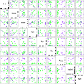
Figure 5: Plots of various globular cluster systems properties and parent galaxy properties. The triangles represent field galaxies and the circles represent cluster galaxies. The names along the diagonal are the variable which is plotted along that particular row and column. Each plot is repeated twice here as the plots in the lower-left triangle and the upper-right triangle represent the same points with the axes inverted.

The moments of the $V-I$ distributions are not well estimated in many of our galaxies based on small numbers of globular clusters. To compare correlations more robustly, we combine the different globular cluster samples to give better estimates of the moments. Because we do not have to exclude galaxies based on there being a small number of measured globular clusters, we now have 43 galaxies in the combined sample. We use the four main parent galaxy properties—magnitude, $\sigma$, Mg2 index, and density environment—for this analysis, breaking the sample into two bins. Figure 5 plots the results for the combined $V-I$ distributions. Table 4 presents the various cuts used for the combined samples and the moments and DIP probability for each sub-sample. Table 4 also presents the number of galaxies and the number of globular clusters in each sub-sample. Each sub–sample has greater than 800 clusters where the noise from the moment estimation is minimal. The choice for the cuts in the sub-samples results from our inspection of the particular distribution; we attempted to find a clear division between the samples, and, when none was apparent, we used cuts which had roughly equal range among the particular variable. The cuts are partly subjective, but the results do not depend strongly on them.

The central location of the $V-I$ peak is statistically different only in the division between faint and bright galaxies. The faint galaxies have a peak around 0.94, and the bright galaxies have a peak around 1.13. For the other divisions, the $V-I$ peaks are similar, but the tail indexes differ significantly. Either faint galaxies, low $\sigma$, low Mg2, or low density cause the $V-I$ distribution to have significantly more tail weight than compared to their counterpart sample.

The most extreme differences between the combined samples results from the DIP probability. Galaxies that are faint, have low $\sigma$ or low Mg2 are consistent with a unimodal distribution, whereas their counterpart samples are highly non-unimodal. This effect is also seen when looking at individual galaxies (see Section 6 above), and it appears to be a fundamental property of galaxies.

8 Discussion

8.1 The Color Distributions

An important discovery in the study of globular clusters systems in the last decade is the fact that the globular clusters’ color distribution of many ellipticals show several peaks (Zepf & Ashman 1993). This property has been interpreted as the presence of several distinct populations of globular clusters around the host galaxy. The origin of these different populations is still under debate and might well have several causes. The original explanation argues that spiral–spiral mergers provide old globular clusters from the progenitors as well as produce a new population during the merger (Ashman & Zepf 1992, see also Schweizer 1987). However, the accretion of enough dwarf galaxies with metal poor clusters will also obviously build up a distinct metal–poor population. Côté et al. (1998), and Hilker (1999) investigated this idea. Yet another process involves the pre–galactic formation of metal–poor clusters as the building blocks of galaxies, followed by the formation of more metal–rich globular clusters during the collapse of the galaxy (see Kissler-Patig 1997, and Kissler-Patig et al. 1998a). Only slightly different is the theory that galaxies formed all their globular clusters in situ and had two main phases of star formation (e.g. Forbes et al. 1997, Harris et al. 1998, Harris et al. 1999). Today’s challenge is to discriminate between the various scenarios with detailed comparison to the present data.

The diversity of the color distributions present in our sample indicates that indeed the scenario is complex. We discuss in turn some of the groups:

$\bullet$ Galaxies that host “only red clusters”—i.e., those having a red peak and a small scale value. The existence of a blue population in these galaxies is not excluded but is unlikely to be significant. The favored scenario for these galaxies is that a single dominant collapse created a bulge and a red population of clusters. We cannot rule the accretion scenario out if these galaxies were formed in an environment poor in material suitable for accretion (e.g. dwarf galaxies, cf. Chapelon 1999). These galaxies would then be in low density environments or in the outskirts of clusters; neither is confirmed nor ruled out by our present statistics. Finally, the merger scenario could also work for these galaxies if the progenitors were poor in blue clusters. If the merger happened at early times, the progenitors could be still in a gaseous form, or, alternatively, could be low–surface–brightness galaxies for late mergers in the field that host a large amount of gas but apparently few clusters. However, a scenario with gaseous mergers at early times is hard to distinguish from the two-stage in situ scenario.

$\bullet$ Galaxies that host “only blue clusters”—i.e., that have a blue peak and a small scale value. These galaxies do not seem to host a significant population of red (presumably metal–rich) clusters. In this case, none of the above scenarios would easily be able to explain such systems; one would have to advocate the formation of bulge stars without the formation of clusters. More likely is a “blue” red peak, either because the red clusters formed with a low metallicity or because they have a significant younger age (about half as old as the true blue clusters, cf. Kissler-Patig et al. 1998a) that make them appear blue. In these last two cases, all scenarios work, with some preference to the merger scenario in the frame of hierarchical clustering models that predict late mergers in the field.

$\bullet$ Galaxies with broad or bimodal color distributions—i.e., that which presumably host a comparable amount (say within a factor of about 3) of blue and red clusters. These are the cases for which the scenarios described above were designed, and we refer to the respective papers for the pros and cons.

Finally, we note that as long as some information is missing (merger epoch, globular clusters formation mechanisms, faint end of the luminosity function in different environments, etc…), and given the diversity of scenarios, it seems that not always the same mechanism is the dominant one.

8.2 Field and Cluster Systems

Although based on small number statistics, field and cluster early–type galaxies seem to differ in the properties of their globular cluster systems. Whereas cluster galaxies show a correlation between peak value and the galaxy size (as measured by the velocity dispersion), such a relation must be ruled out for field galaxies.

For cluster ellipticals, the recent spectroscopic studies (Cohen et al. 1998, Kissler-Patig et al. 1998b) show that all globular clusters are old (around 10 Gyr or older). At these ages, the clusters can be considered coeval with respect to the influence of their ages on color. Color differences can therefore be interpreted as almost pure metallicity differences, and the relation between peak color and galaxy luminosity might reflect the equivalent of the Mg2–$\sigma$ relation for galaxies. Forbes et al. (1997) suggest that in systems with two distinct globular cluster populations, the mean metallicity of the red clusters correlates with the luminosity of the host galaxy; the blue peak does not. Their conclusion implies that the correlation of the total sample’s mean color with galaxy size is driven by the metal–rich globular clusters only. Consequently, this would support scenarios in which the metal–poor globular clusters formed in events uncorrelated with their future host galaxy—e.g., in systems that are separate entities from their future hosts. On the other hand, the same research suggests that the metal–rich globular clusters formed in events correlated with the future host galaxy—e.g., the formation of a bulge in a collapse or merger event. In addition, this correlation suggests that the blue sub–populations have roughly a constant color, while for the red population both the peak shifts and the scale increase as a function of color.

Perhaps surprisingly, the peak color of globular clusters in field galaxies does not correlate with the velocity dispersion ($\approx$ size) of their host galaxy. This result appears to be in contrast with the observation that field and cluster galaxies do exhibit the same Mg2–$\sigma$ relations (Bernardi et al. 1998). We see several possible explanations.

A first alternative might be that the correlation for cluster galaxies is artificial. We verified that it is not caused by sampling different regions in the different galaxies. Indeed, the ratio of blue to red galaxies does vary with radius (Geisler et al. 1997, Kissler-Patig et al. 1997b, Puzia et al. 1999). Furthermore, the WFPC2 field samples the outer parts less in larger galaxies than in small ones, so that the relative ratio of blue to red galaxies is systematically smaller in large galaxies at fixed field of view. Puzia et al. (1999) tested the importance of this effect on NGC 4472, which has exposures centered on the galaxy as well as several arcminute offsets north and south. The respective peaks of the blue and red populations do not change with radius within the errors; however, the varying ratio of blue to red causes the overall peak to shift by 0.02 mag from the inner to the outer field. The effect is too small, though, to explain any systematic correlation. Moreover, in our sample, field and cluster galaxies span different values of galaxy $\sigma$. Where cluster galaxies are of intermediate to giant size, the field galaxies span the low to intermediate size range. If indeed intermediate and giant early–type galaxies differ (see above, cf. Kissler-Patig 1997), the presence/absence of a correlation would be due not to environment, but rather to a function of the galaxy size. For example, one could speculate that small galaxies are not surrounded by a “halo” of blue clusters, thus showing a small trend of system peak with size. Intermediate size or larger galaxies might or might not have such a halo of blue clusters, complicating the interpretation of the peak color and introducing a scatter due to the possible existence of blue clusters. Giant ellipticals would always have blue clusters, and a significant redder population that correlates with galaxy size, leading to an overall trend of peak color with galaxy size again. In other words, the correlation would be an artifact of the mix of populations which show a correlation with environment, rather than a physical difference in the enrichment histories.

A second alternative would be a physical interpretation of the result. Thus, the presence of a Mg2–$\sigma$ relations in field and cluster galaxies, but absence/presence respectively of a peak–$\sigma$ relation, would indicate that stars and globular clusters are coupled in cluster galaxies but not in field galaxies. We regard this alternative as unlikely, however, since cluster formation and star formation appear to go together.

Finally, Mg2 and $V-I$ color could vary differently with age and metallicity. The variations of Mg2 with age and metallicity are still uncertain and if, for example, the metal–rich population in field ellipticals show a large spread in age from galaxy to galaxy, a trend could mimic an Mg2–$\sigma$ relation in the field but not a peak–$\sigma$ relation. In contrast, since all globular clusters in cluster galaxies are old, such a trend would not be present, and both Mg2 and peak would trace metallicity only. Clearly such speculations require a much better understanding of the influence of age and metallicity on the properties of composite stellar populations. Detailed studies of the ages and metallicities of the systems are needed.

9 Summary and Outlook

The results presented in this paper suggest that we can use globular cluster systems to study the merger/formation history of both itself and its host galaxy. The differences we see between the field and cluster systems suggest that the cluster galaxies are more influenced by accretion, whereas the field systems may be the result of “in situ” globular cluster formation. Combining this result with the strong signature of multi-modality seen in many of the systems provides an observational comparison to the various formation scenarios. In a companion paper (Côté et al. 2000), we will compare these results to the theoretical predictions of Côté et al. (1998). More detailed studies of the systems that are candidates for bimodal distributions are underway, including follow–up near–infrared photometry and multi–object spectroscopy.

All photometry results are available from the authors.

Table 1: Observational Parameters

Galaxy	Filter	Texp	Nexp	PI (number)
N0584	F555W	1520	5	Faber (6099)
	F814W	1450	7	Faber (6099)
N0596	F555W	1600	4	Richstone (6587)
	F814W	1800	3	Richstone (6587)
N0821	F555W	1520	5	Faber (6099)
	F814W	1450	7	Faber (6099)
N1023a	F555W	2920	11	Faber,Richstone (6099,6587)
	F814W	3780	10	Faber,Richstone (6099,6587)
N1316	F450W	5000	5	Grillmair (5990)
	F814W	1860	3	Grillmair (5990)
N1399	F450W	5200	4	Grillmair (5990)
	F814W	1800	3	Grillmair (5990)
N1404	F450W	5000	5	Grillmair (5990)
	F814W	1860	3	Grillmair (5990)
N1426	F555W	1600	4	Richstone (6587)
	F814W	1800	3	Richstone (6587)
N1700	F555W	1600	4	Richstone (6587)
	F814W	1800	3	Richstone (6587)
N2300	F555W	1520	5	Faber (6099)
	F814W	1450	7	Faber (6099)
N2434	F555W	1300	2	Carollo (5943)
	F814W	1000	2	Carollo (5943)
N2778	F555W	1520	5	Faber (6099)
	F814W	1450	7	Faber (6099)
N3115	F555W	1015	6	Faber (5512)
	F814W	1236	6	Faber (5512)
N3377	F555W	1330	6	Faber (5512)
	F814W	1236	6	Faber (5512)
N3379	F555W	1660	4	Faber (5512)
	F814W	1340	4	Faber (5512)
N3384	F555W	1430	6	Faber (5512)
	F814W	1290	6	Faber (5512)
N3585	F555W	1200	6	Richstone (6587)
	F814W	1900	3	Richstone (6587)
N3610	F555W	1400	6	Richstone (6587)
	F814W	2100	3	Richstone (6587)
N3640	F555W	1200	6	Richstone (6587)
	F814W	2100	3	Richstone (6587)
N4125	F555W	1400	6	Faber (6587)
	F814W	2100	3	Faber (6587)
N4192	F555W	660	3	Rubin (5375)
	F814W	660	3	Rubin (5375)
N4291	F555W	1520	5	Faber (6099)
	F814W	1450	7	Faber (6099)
N4343	F555W	660	3	Rubin (5375)
	F814W	660	3	Rubin (5375)
N4365	F555W	2200	2	Brodie (5920)
	F814W	2300	2	Brodie (5920)
N4374	F547M	1200	2	Bower (6094)
	F814W	520	2	Bower (6094)
N4406	F555W	1500	3	Faber (5512)
	F814W	1500	3	Faber (5512)
N4450	F555W	520	3	Rubin (5375)
	F814W	520	3	Rubin (5375)
N4458	F555W	1340	4	Faber (5512)
	F814W	1120	5	Faber (5512)
N4472a	F555W	4400	4	Brodie (5920)
	F814W	4600	4	Brodie (5920)
N4473	F555W	1800	3	Faber (6099)
	F814W	2000	4	Faber (6099)
N4478	F555W	1600	4	Richstone (6587)
	F814W	1800	3	Richstone (6587)
N4486	F555W	2810	6	Macchetto (5477)
	F814W	2430	5	Macchetto (5477)
N4486B	F555W	1800	3	Faber (6099)
	F814W	2000	4	Faber (6099)
N4526	F555W	520	3	Rubin (5375)
	F814W	520	3	Rubin (5375)
N4536	F555W	660	3	Rubin (5375)
	F814W	660	3	Rubin (5375)
N4550	F555W	1200	3	Rubin (5375)
	F814W	1200	3	Rubin (5375)
N4552	F555W	2400	4	Faber (6099)
	F814W	1500	3	Faber (6099)
N4569	F555W	520	3	Rubin (5375)
	F814W	520	3	Rubin (5375)
N4594	F547M	1340	4	Faber (5512)
	F814W	1470	6	Faber (5512)
N4621	F555W	1380	6	Faber (5512)
	F814W	1280	6	Faber (5512)
N4649	F555W	2100	2	Westphal (6286)
	F814W	2500	2	Westphal (6286)
N4660	F555W	1000	5	Faber (5512)
	F814W	850	5	Faber (5512)
N4881	F555W	7200	8	Westphal (5233)
	F814W	7200	8	Westphal (5233)
N5018	F555W	1200	6	Richstone (6587)
	F814W	1900	3	Richstone (6587)
N5061	F555W	1200	6	Richstone (6587)
	F814W	1900	3	Richstone (6587)
N5845	F555W	2140	5	Faber (6099)
	F814W	1120	5	Faber (6099)
N5846a	F555W	6600	6	Brodie (5920)
	F814W	6900	6	Brodie (5920)
N7192	F555W	1300	2	Carollo (5943)
	F814W	1000	2	Carollo (5943)
N7457	F555W	1380	6	Faber (5512)
	F814W	1280	6	Faber (5512)
IC4889	F555W	600	1	Carollo (5943)
	F814W	600	1	Carollo (5943)

Table 2: Galaxy Properties

Galaxy	Type	$M_{V}$	log($\sigma$)	Mg2	log($\rho$)	a4	log(Re)(pc)
N584	E4	–21.16	2.34	0.29	0.42	1.50	3.51
N596	Epec	–20.93	2.22	0.25	0.40	1.30	$\cdots$
N821	E6	–20.84	2.32	0.32	0.08	2.50	3.45
N1023	SB0	–20.61	2.34	0.34	0.57	$\cdots$	3.26
N1399	E1pec	–21.97	2.52	0.37	1.59	0.00	$\cdots$
N1404	E1	–21.56	2.38	0.34	1.59	0.50	$\cdots$
N1426	E4	–20.42	2.18	0.28	0.66	$\cdots$	3.44
N1700	E4	–21.90	2.36	0.28	$\cdots$	0.90	$\cdots$
N2300	SA0	–20.76	2.42	0.33	0.14	–0.60	3.58
N2434	E0	–20.60	2.31	0.27	0.19	$\cdots$	3.49
N2778	E	–19.43	2.26	0.34	0.28	$\cdots$	$\cdots$
N3115	S0	–20.82	2.45	0.34	0.08	8.00	3.17
N3377	E5	–19.96	2.18	0.29	0.49	1.20	3.21
N3379	E1	–20.83	2.35	0.34	0.52	0.10	3.23
N3384	SB0	–19.89	2.21	0.29	0.54	$\cdots$	$\cdots$
N3585	E7	–21.75	2.34	0.32	0.12	4.50	3.50
N3610	E5	–20.92	2.21	0.27	0.30	2.50	$\cdots$
N3640	E3	–21.75	2.24	0.27	0.18	–0.20	$\cdots$
N4125	E6pec	–22.09	2.25	0.32	0.34	1.00	3.43
N4291	E	–20.69	2.43	0.32	0.36	–0.40	3.64
N4365	E3	–22.12	2.42	0.35	2.93	–1.10	3.79
N4374	E1	–22.21	2.44	0.32	3.99	–0.40	$\cdots$
N4406	S0	–22.41	2.40	0.33	1.41	–0.70	$\cdots$
N4458	E0	–19.06	2.02	0.25	3.21	$\cdots$	$\cdots$
N4472	E2	–22.59	2.48	0.34	3.31	–0.30	3.89
N4473	E5	–20.80	2.26	0.33	2.17	0.90	3.60
N4478	E2	–19.94	2.13	0.27	3.92	–0.80	$\cdots$
N4486	E0	–22.48	2.56	0.30	4.17	0.00	3.89
N4486b	cE0	–17.75	2.30	0.30	4.17	$\cdots$	3.51
N4526	SAB0	–20.89	2.47	0.30	2.45	$\cdots$	3.57
N4550	SB0	–18.81	2.01	0.17	2.97	–0.70	$\cdots$
N4552	E	–21.26	2.42	0.35	2.97	$\cdots$	3.35
N4621	E5	–21.63	2.40	0.35	2.60	1.50	3.54
N4649	E2	–22.31	2.56	0.37	3.49	–0.50	3.74
N4660	E	–19.26	2.29	0.33	3.37	2.70	3.56
N4881	E	–21.60	2.33	0.29	$\cdots$	$\cdots$	$\cdots$
N5018	E3	–22.31	2.32	0.21	0.29	2.00	$\cdots$
N5061	E0	–21.62	2.30	0.27	0.31	–1.80	3.90
N5845	E	–19.63	2.42	0.32	0.84	0.80	$\cdots$
N5846	E0	–22.23	2.40	0.34	0.84	0.00	3.37
N7192	SA0	–21.49	2.27	0.26	0.28	$\cdots$	3.71
N7457	SA0	–18.25	1.76	0.19	0.13	$\cdots$	$\cdots$
IC4889	E5	–21.26	2.22	0.26	0.13	1.00	$\cdots$

Table 3: Moments of $V-I$ Distributions

Galaxy	NGC	$V-I$ peak	Scale	Skewness	Tail	DIP
N584	67	$1.092~{}_{1.062}^{1.123}$	$0.159~{}_{0.130}^{0.192}$	$-0.013~{}_{-1.159}^{+1.128}$	$1.080~{}_{0.864}^{1.484}$	$0.649~{}_{0.500}^{0.852}$
N596	31	$1.049~{}_{1.004}^{1.096}$	$0.158~{}_{0.115}^{0.201}$	$+0.306~{}_{-0.981}^{+1.541}$	$1.176~{}_{0.833}^{2.049}$	$0.661~{}_{0.500}^{0.778}$
N821	55	$1.008~{}_{0.976}^{1.041}$	$0.142~{}_{0.126}^{0.158}$	$+0.257~{}_{-1.006}^{+1.518}$	$0.805~{}_{0.690}^{0.980}$	$0.785~{}_{0.500}^{0.840}$
N1023	149	$1.037~{}_{1.010}^{1.063}$	$0.198~{}_{0.172}^{0.229}$	$+1.660~{}_{+0.271}^{+2.953}$	$1.007~{}_{0.878}^{1.401}$	$0.635~{}_{0.500}^{0.696}$
N1316	186	$0.966~{}_{0.951}^{0.981}$	$0.130~{}_{0.114}^{0.149}$	$-1.001~{}_{-2.382}^{+0.499}$	$1.196~{}_{0.971}^{1.479}$	$0.500~{}_{0.500}^{0.590}$
N1399	410	$1.051~{}_{1.040}^{1.063}$	$0.124~{}_{0.118}^{0.130}$	$-4.387~{}_{-6.649}^{-2.187}$	$0.886~{}_{0.784}^{0.998}$	$0.968~{}_{0.908}^{0.969}$
N1404	138	$1.017~{}_{0.999}^{1.037}$	$0.137~{}_{0.125}^{0.152}$	$+0.125~{}_{-1.470}^{+1.741}$	$0.770~{}_{0.693}^{0.878}$	$0.995~{}_{0.886}^{0.995}$
N1426	74	$1.084~{}_{1.050}^{1.118}$	$0.176~{}_{0.153}^{0.198}$	$+0.486~{}_{-0.673}^{+1.660}$	$0.965~{}_{0.817}^{1.205}$	$0.995~{}_{0.705}^{1.000}$
N1700	27	$1.122~{}_{1.059}^{1.187}$	$0.213~{}_{0.163}^{0.292}$	$+1.328~{}_{+0.034}^{+2.416}$	$1.093~{}_{0.778}^{1.937}$	$0.500~{}_{0.500}^{0.743}$
N2300	82	$1.071~{}_{1.031}^{1.110}$	$0.193~{}_{0.168}^{0.222}$	$+0.881~{}_{-0.377}^{+2.135}$	$0.911~{}_{0.772}^{1.110}$	$0.500~{}_{0.500}^{0.675}$
N2434	143	$0.945~{}_{0.922}^{0.968}$	$0.189~{}_{0.156}^{0.224}$	$+0.465~{}_{-0.723}^{+1.706}$	$1.100~{}_{0.875}^{1.473}$	$0.598~{}_{0.500}^{0.798}$
N2778	18	$1.072~{}_{1.007}^{1.143}$	$0.213~{}_{0.138}^{0.306}$	$-0.827~{}_{-2.033}^{+0.597}$	$1.291~{}_{0.772}^{2.567}$	$0.595~{}_{0.500}^{0.800}$
N3115	94	$1.030~{}_{1.002}^{1.058}$	$0.167~{}_{0.146}^{0.190}$	$+1.363~{}_{+0.119}^{+2.652}$	$0.933~{}_{0.773}^{1.119}$	$0.709~{}_{0.500}^{0.754}$
N3377	86	$1.072~{}_{1.047}^{1.095}$	$0.141~{}_{0.118}^{0.169}$	$-0.680~{}_{-1.905}^{+0.523}$	$1.017~{}_{0.826}^{1.250}$	$0.500~{}_{0.500}^{0.779}$
N3379	52	$1.095~{}_{1.054}^{1.129}$	$0.172~{}_{0.142}^{0.208}$	$+0.896~{}_{-0.307}^{+2.078}$	$0.950~{}_{0.728}^{1.317}$	$0.500~{}_{0.500}^{0.770}$
N3384	39	$1.023~{}_{0.969}^{1.084}$	$0.204~{}_{0.157}^{0.261}$	$+1.248~{}_{+0.058}^{+2.285}$	$1.067~{}_{0.746}^{1.640}$	$0.500~{}_{0.500}^{0.737}$
N3585	70	$1.110~{}_{1.071}^{1.149}$	$0.202~{}_{0.173}^{0.239}$	$+0.331~{}_{-0.971}^{+1.564}$	$0.993~{}_{0.805}^{1.276}$	$0.500~{}_{0.500}^{0.768}$
N3610	29	$1.105~{}_{1.044}^{1.182}$	$0.191~{}_{0.149}^{0.245}$	$+0.154~{}_{-1.102}^{+1.467}$	$0.956~{}_{0.747}^{1.513}$	$0.996~{}_{0.557}^{1.000}$
N3640	48	$1.080~{}_{1.045}^{1.116}$	$0.158~{}_{0.132}^{0.186}$	$+0.982~{}_{-0.250}^{+2.125}$	$0.852~{}_{0.697}^{1.283}$	$0.971~{}_{0.593}^{0.994}$
N4125	68	$1.001~{}_{0.954}^{1.042}$	$0.218~{}_{0.185}^{0.251}$	$+0.241~{}_{-1.019}^{+1.560}$	$1.007~{}_{0.784}^{1.378}$	$0.500~{}_{0.500}^{0.814}$
N4192	49	$0.884~{}_{0.804}^{0.970}$	$0.366~{}_{0.306}^{0.425}$	$+0.179~{}_{-0.910}^{+1.268}$	$0.888~{}_{0.680}^{1.254}$	$0.500~{}_{0.500}^{0.668}$
N4291	71	$0.983~{}_{0.952}^{1.016}$	$0.161~{}_{0.138}^{0.187}$	$+0.637~{}_{-0.561}^{+1.770}$	$1.072~{}_{0.865}^{1.348}$	$0.500~{}_{0.500}^{0.941}$
N4343	25	$1.026~{}_{0.962}^{1.096}$	$0.246~{}_{0.137}^{0.325}$	$+0.586~{}_{-0.622}^{+1.667}$	$1.442~{}_{0.863}^{2.543}$	$0.500~{}_{0.500}^{0.827}$
N4365	409	$1.094~{}_{1.079}^{1.111}$	$0.188~{}_{0.175}^{0.203}$	$+0.253~{}_{-1.335}^{+1.851}$	$0.941~{}_{0.859}^{1.047}$	$0.757~{}_{0.514}^{0.795}$
N4374	123	$0.999~{}_{0.977}^{1.021}$	$0.151~{}_{0.133}^{0.171}$	$+2.025~{}_{+0.560}^{+3.285}$	$0.909~{}_{0.773}^{1.111}$	$0.520~{}_{0.500}^{0.690}$
N4406	131	$1.041~{}_{1.021}^{1.059}$	$0.132~{}_{0.119}^{0.146}$	$+0.283~{}_{-1.347}^{+1.730}$	$0.777~{}_{0.690}^{0.923}$	$0.500~{}_{0.500}^{0.571}$
N4450	29	$0.941~{}_{0.850}^{1.017}$	$0.284~{}_{0.189}^{0.373}$	$-0.278~{}_{-1.476}^{+0.889}$	$1.360~{}_{0.867}^{2.018}$	$0.500~{}_{0.500}^{0.768}$
N4458	33	$1.071~{}_{0.982}^{1.139}$	$0.221~{}_{0.127}^{0.270}$	$+0.887~{}_{-0.380}^{+1.970}$	$0.928~{}_{0.556}^{1.937}$	$0.698~{}_{0.500}^{0.764}$
N4472	486	$1.095~{}_{1.078}^{1.113}$	$0.250~{}_{0.232}^{0.269}$	$-0.236~{}_{-1.865}^{+1.308}$	$0.985~{}_{0.905}^{1.087}$	$0.997~{}_{0.945}^{0.997}$
N4473	112	$1.026~{}_{1.003}^{1.050}$	$0.149~{}_{0.134}^{0.168}$	$-0.618~{}_{-1.992}^{+0.983}$	$0.896~{}_{0.765}^{1.052}$	$0.500~{}_{0.500}^{0.667}$
N4478	50	$1.060~{}_{1.022}^{1.100}$	$0.166~{}_{0.136}^{0.206}$	$+0.267~{}_{-1.054}^{+1.492}$	$1.017~{}_{0.797}^{1.402}$	$0.614~{}_{0.500}^{0.744}$
N4486	655	$1.108~{}_{1.097}^{1.118}$	$0.158~{}_{0.151}^{0.164}$	$+0.290~{}_{-2.404}^{+2.615}$	$0.821~{}_{0.764}^{0.881}$	$0.978~{}_{0.951}^{0.978}$
N4486b	87	$0.978~{}_{0.953}^{1.001}$	$0.142~{}_{0.117}^{0.175}$	$+0.501~{}_{-0.746}^{+1.678}$	$1.038~{}_{0.844}^{1.491}$	$0.500~{}_{0.500}^{0.767}$
N4526	75	$1.030~{}_{0.988}^{1.074}$	$0.214~{}_{0.186}^{0.248}$	$-0.243~{}_{-1.480}^{+0.993}$	$0.815~{}_{0.644}^{1.037}$	$0.999~{}_{0.500}^{0.999}$
N4536	87	$0.766~{}_{0.691}^{0.847}$	$0.388~{}_{0.332}^{0.439}$	$+2.334~{}_{+0.951}^{+3.478}$	$1.042~{}_{0.836}^{1.329}$	$0.500~{}_{0.500}^{0.840}$
N4550	37	$1.020~{}_{0.944}^{1.098}$	$0.305~{}_{0.254}^{0.363}$	$+0.022~{}_{-1.115}^{+1.218}$	$0.909~{}_{0.700}^{1.238}$	$0.500~{}_{0.500}^{0.688}$
N4552	171	$1.062~{}_{1.043}^{1.083}$	$0.156~{}_{0.142}^{0.171}$	$+1.121~{}_{-0.354}^{+2.603}$	$0.959~{}_{0.851}^{1.094}$	$0.500~{}_{0.500}^{0.707}$
N4569	67	$0.816~{}_{0.748}^{0.885}$	$0.347~{}_{0.309}^{0.390}$	$+0.492~{}_{-0.798}^{+1.667}$	$0.988~{}_{0.807}^{1.181}$	$0.973~{}_{0.554}^{0.988}$
N4594	122	$1.065~{}_{1.042}^{1.089}$	$0.152~{}_{0.130}^{0.176}$	$-1.988~{}_{-3.310}^{-0.430}$	$0.848~{}_{0.687}^{1.121}$	$0.995~{}_{0.627}^{1.000}$
N4621	126	$1.079~{}_{1.059}^{1.099}$	$0.128~{}_{0.116}^{0.141}$	$-1.611~{}_{-3.073}^{-0.130}$	$0.916~{}_{0.773}^{1.119}$	$0.539~{}_{0.500}^{0.654}$
N4649	378	$1.096~{}_{1.081}^{1.111}$	$0.185~{}_{0.171}^{0.200}$	$-1.401~{}_{-2.909}^{+0.251}$	$0.867~{}_{0.794}^{0.946}$	$0.961~{}_{0.810}^{0.963}$
N4660	74	$0.962~{}_{0.935}^{0.992}$	$0.148~{}_{0.117}^{0.183}$	$+0.899~{}_{-0.330}^{+2.148}$	$1.091~{}_{0.832}^{1.445}$	$0.500~{}_{0.500}^{0.767}$
N4881	84	$0.915~{}_{0.868}^{0.959}$	$0.276~{}_{0.225}^{0.337}$	$+0.505~{}_{-0.497}^{+1.683}$	$1.321~{}_{1.026}^{1.770}$	$0.500~{}_{0.500}^{0.999}$
N5018	10	$0.931~{}_{0.848}^{1.013}$	$0.187~{}_{0.111}^{0.309}$	$+0.193~{}_{-1.145}^{+1.340}$	$1.714~{}_{0.965}^{3.228}$	$0.500~{}_{0.500}^{0.773}$
N5061	84	$1.099~{}_{1.068}^{1.127}$	$0.190~{}_{0.143}^{0.242}$	$-0.473~{}_{-1.602}^{+0.723}$	$1.231~{}_{0.907}^{1.812}$	$0.500~{}_{0.500}^{0.800}$
N5845	28	$1.127~{}_{1.044}^{1.215}$	$0.285~{}_{0.211}^{0.364}$	$+0.543~{}_{-0.617}^{+1.569}$	$1.272~{}_{0.878}^{1.851}$	$0.500~{}_{0.500}^{0.733}$
N5846	781	$1.080~{}_{1.066}^{1.094}$	$0.249~{}_{0.232}^{0.266}$	$-2.895~{}_{-4.551}^{-1.318}$	$1.167~{}_{1.070}^{1.261}$	$0.895~{}_{0.692}^{0.935}$
N7192	95	$1.068~{}_{1.029}^{1.112}$	$0.262~{}_{0.215}^{0.313}$	$-0.196~{}_{-1.338}^{+0.990}$	$1.115~{}_{0.882}^{1.446}$	$0.500~{}_{0.500}^{0.810}$
N7457	48	$1.024~{}_{0.991}^{1.056}$	$0.147~{}_{0.113}^{0.206}$	$+0.673~{}_{-0.461}^{+1.802}$	$1.288~{}_{0.857}^{2.449}$	$0.500~{}_{0.500}^{0.770}$
IC4889	48	$1.024~{}_{0.992}^{1.056}$	$0.147~{}_{0.113}^{0.203}$	$+0.673~{}_{-0.530}^{+1.800}$	$1.288~{}_{0.875}^{2.521}$	$0.500~{}_{0.500}^{0.800}$

Table 4: Moments of Combined Samples

Sub-Sample	Range	NG	NGC	$V-I$ peak	Scale	Skewness	Tail	DIP
Faint	M${}_{V}>-20.70$	15	803	$1.019~{}_{1.008}^{1.029}$	$0.182~{}_{0.173}^{0.192}$	$+1.663~{}_{+0.302}^{+3.005}$	$1.001~{}_{0.941}^{1.065}$	$0.742~{}_{0.500}^{0.815}$
Bright	M${}_{V}<-21.75$	13	2737	$1.077~{}_{1.072}^{1.083}$	$0.172~{}_{0.168}^{0.176}$	$-1.397~{}_{-3.383}^{+0.518}$	$0.884~{}_{0.857}^{0.913}$	$0.954~{}_{0.781}^{0.963}$
Low $\sigma$	log$(\sigma)<2.3$	16	872	$1.041~{}_{1.031}^{1.051}$	$0.188~{}_{0.178}^{0.197}$	$+1.243~{}_{-0.118}^{+2.509}$	$1.022~{}_{0.964}^{1.080}$	$0.759~{}_{0.500}^{0.904}$
High $\sigma$	log$(\sigma)>2.4$	12	2992	$1.075~{}_{1.070}^{1.080}$	$0.173~{}_{0.169}^{0.177}$	$-0.455~{}_{-2.586}^{+1.662}$	$0.879~{}_{0.855}^{0.907}$	$0.996~{}_{0.959}^{0.996}$
Low Mg2	Mg2 $<0.30$	18	1496	$1.069~{}_{1.061}^{1.078}$	$0.205~{}_{0.197}^{0.214}$	$-0.104~{}_{-1.894}^{+1.786}$	$1.039~{}_{0.987}^{1.094}$	$0.791~{}_{0.562}^{0.851}$
High Mg2	Mg2 $>0.34$	15	2597	$1.070~{}_{1.064}^{1.075}$	$0.170~{}_{0.166}^{0.175}$	$-0.292~{}_{-2.258}^{+1.618}$	$0.888~{}_{0.859}^{0.916}$	$0.985~{}_{0.936}^{0.985}$
Low $\rho$	log$(\rho)<1.0$	24	2202	$1.057~{}_{1.050}^{1.064}$	$0.200~{}_{0.194}^{0.207}$	$+1.306~{}_{-0.364}^{+2.994}$	$1.019~{}_{0.977}^{1.057}$	$0.967~{}_{0.780}^{0.974}$
High $\rho$	log$(\rho)>1.0$	17	3441	$1.069~{}_{1.064}^{1.074}$	$0.170~{}_{0.166}^{0.173}$	$-0.262~{}_{-2.304}^{+1.903}$	$0.887~{}_{0.862}^{0.909}$	$0.999~{}_{0.948}^{0.999}$

Figure 1: Histogram of the globular cluster system’s $V-I$ colors for all of the galaxies. The solid line represents a density estimate and the dotted lines are the 90% confidence bands. The total number of globular clusters appears under the galaxy name.

Figure 1: continued.

Figure 1: continued.

Figure 1: continued.

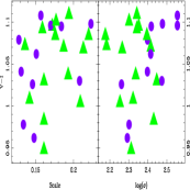
Figure 6: Scale and log($\sigma$) versus the $V-I$ color of the globular cluster systems. The colors of the points represent the same as in the previous plot.

Figure 7: The distribution of the DIP probability with it’s 68% confidence band for all of the galaxies. The DIP probability is bounded by 0.5 and 1.0.

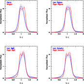
Figure 8: $V-I$ distributions and their 90% confidence bands for the globular clusters combined across galaxies; we use two bins for each of the named galaxy properties. Each curve represents an adaptive kernel estimate of the density with unity area.

References

- (1) Ashman, K.M., & Zepf, S.E. 1992, ApJ, 384, 50
- (2) Ashman, K.M., & Zepf, S.E. 1998, “Globular Cluster Systems”, Cambridge University Press (Cambridge astrophysics series, 30)
- (3) Baugh, C.M., Cole, S., Frenk, C.S. 1996, MNRAS, 283, 1361
- (4) Beers, T., Flynn, K., & Gebhardt, K. 1991, AJ, 100, 32
- (5) Bernardi, M., Renzini, A., Da Costa, L., Wegner, G., Alonso, M., Pellegrini, P., Rité, C., & Willmer, C. 1998, ApJ, 508, 143
- (6) Bertin, E., & Arnouts, S. 1996, A&AS, 117, 393
- (7) Bird, T., & Beers, T. 1993, AJ, 105, 1596
- (8) Bruzual, A., & Charlot, S. 1993, ApJ, 405, 538
- (9) Chapelon, S. 1999, in press
- (10) Cohen, J., Blakeslee, J., & Ryzhov, A. 1998, ApJ, 496, 808
- (11) Côté, P., Marzke, R., & West, M. 1998, ApJ, 501, 554
- (12) Côté, P., et al. 2000, in preparation
- (13) Elson, R., & Santiago, B. 1996, MNRAS, 280, 971
- (14) Forbes, D., Brodie, J., & Huchra, J. 1997, AJ, 113, 887
- (15) Forbes, D., Grillmair, C., Williger, G., Elson, R., & Brodie, J. 1998, MNRAS, 293, 325
- (16) Geisler, D., Lee, M., & Kim, E. 1996, AJ, 111, 1529
- (17) Harris, G.L.H., Harris, W.E., & Poole, G.B. 1999, AJ, 117, 855
- (18) Harris, W.E. 1991, ARA&A, 29, 543
- (19) Harris, W.E., Harris, G.L.H., & McLaughlin, D.E. 1998, AJ, 115, 1801
- (20) Hartigan, J.A., & Hartigan, P.M. 1985, Ann. Statist.,13, 70
- (21) Hilker, M., Infante, L., & Richtler, T. 1999, astro-ph/9905112
- (22) Holtzman, J., Burrows, C., Casertano, S., Hester, J., Trauger, J., Watson, A., & Worthey, G. 1995, PASP, 107, 1065
- (23) Kauffmann, G. 1996, MNRAS, 281, 487
- (24) Kissler-Patig, M. 1997, A&A, 319, 83
- (25) Kissler-Patig, M., Kohle, S., Hilker, M., Richtler, T., Infante, L., & Quintana, H. 1997a, A&A, 319, 470
- (26) Kissler-Patig, M., Richtler, T., Storm, J., & Della Valle, M. 1997b, A&A, 327, 503
- (27) Kissler-Patig, M., Forbes, D., & Minniti, D. 1998a, MNRAS, 298, 1123
- (28) Kissler-Patig, M., Brodie, J., Schroder, L., Forbes, D., Grillmair, C., & Huchra, J. 1998b, AJ, 115, 105
- (29) Kissler-Patig, M., Brodie, J.P., & Minniti, D. 1999, in preparation
- (30) Kundu, A., & Whitmore, B. 1998, AJ, 116, 2841
- (31) Neilsen, E., & Tsvetanov, Z. 1999, astro-ph 9902164
- (32) Ostrov, P., Forte, J., & Geisler, D. 1998, AJ, 116, 2854
- (33) Puzia, T., Kissler-Patig, M., & Brodie, J. 1999, submitted AJ
- (34) Schindler, S., Binggeli, B., & Böhringer, H. 1999, A&A, 343, 420
- (35) Schlegel, D., Finkbeiner, D., & Davis, M. 1998, ApJ, 500, 525
- (36) Silverman, B.W., 1986, Density Estimation for Statistics and Data Analysis (New York: Chapman and Hall)
- (37) Whitmore, B., Sparks, W., Lucas, R., Macchetto, R., & Biretta, J. 1995, ApJ, 454, L73
- (38) Whitmore, B.C., Miller, B.W., Schweizer, F., & Fall, S.M. 1997, AJ, 114, 1797
- (39) Williams, R.E., et al. 1996, AJ, 112, 1335
- (40) Worthey, G. 1994, ApJS, 95, 107
- (41) Zepf, S.E., & Ashman, K.M. 1993, MNRAS, 264, 611