The $b$ Distribution of the Ly$\alpha$ Forest: Probing Cosmology and the Intergalactic Medium

Abstract

We investigate a method to determine the temperature-density relation of the intergalactic medium (IGM) at $z\sim 2-4$ using quasar absorption line systems. Using a simple model combined with numerical simulations we show that there is a lower cutoff in the distribution of column density ($N_{\rm HI}$) and line width ($b$ parameter). The location of this cutoff can be used to determine the temperature-density relation (under certain conditions). We describe and test an algorithm to do this. The method works as long as the amplitude of fluctuations on these scales ($\sim 100$ kpc) is sufficiently large. Models with less power can mimic higher temperatures. A preliminary application is made to data from two quasar lines-of-sight, and we determine an upper limit to the temperature of the IGM. Finally, we examine the full distribution of $b$-parameters and show that this is completely specified by just two parameters: the temperature of the gas and the amplitude of the power spectrum. Using the temperature upper limit measured with the $N_{\rm HI}-b$ cutoff method, we derive an upper limit to the amplitude of the power spectrum.

and

1 Introduction

It has become clear that observations of absorption lines in the spectra of high-redshift quasars can give us valuable information about the nature and distribution of the intergalactic medium. Early theoretical work ([Doroshkevich & Shandarin 1977]; [Rees 1986]; [Bond, Szalay & Silk 1988]; [McGill 1990]; [Bi, Börner & Chu 1992]), supplemented with numerical simulations ([Cen et al. 1994]; [Petitjean, Müket & Kates]; [Zhang et al. 1995]; [Hernquist et al. 1996]) showed convincingly that absorption lines at $z\sim 3$ with column densities less than about $10^{16}$ cm^-2 arise primarily from a network of relatively low density filaments and sheets that naturally form out of hierarchical primordial perturbations.

Having established the link between cosmology and the Ly$\alpha$ forest, subsequent work has focused on two related areas: improving our understanding of the physical conditions of the IGM (at these redshifts), and using the forest to constrain cosmological parameters. This includes using the power spectrum of the flux distribution ([Croft et al. 1998]; [Croft, Hu & Davé 1999]), the slope of the column density distribution ([Hui, Gnedin & Zhang 1997]; [Gnedin 1998]; [Machacek et al. 1999]), and inverting the flux-density relation ([Nusser & Haehnelt 1999]).

Although early simulations seemed to show that all models were in agreement with observations, recently it was shown ([Theuns et al. 1998]; [Bryan et al. 1999]), that the width of the absorbers, commonly quantified by the $b$ parameter of a Voigt-profile, had been over-predicted in most previous work. This left a discrepancy between the canonical model and the observations.

A number of ways to resolve this have been suggested, mostly revolving around ways to increase the temperature of the gas, and hence the width of the lines. The low density gas in the IGM is very close to photoionization equilibrium with a background radiation field, usually assumed to be from quasars. Its temperature is determined by a competition between adiabatic cooling and photo-ionization heating ([Hui & Gnedin 1997]). An increase in the density will result in more photo-ionization heating and hence higher temperatures. In Theuns et al. (1999)the99, it was shown that increasing $\Omega_{b}$, the ratio of the baryon density to the critical density, could widen the lines. However, even after doubling the baryon density to the edge of that permitted by primordial nucleosynthesis, they still found some disagreement. Along similar lines, delaying helium reionization to $z\sim 3-4$ ([Haehnelt & Steinmetz 1998]) can provide a small boost in the temperature.

In part driven by this discrepancy, there have been some recent suggestions on other ways to increase the temperature of the IGM. The first is a suggestion of Compton heating from a hard X-ray background ([Madau & Efstathiou 1999]). The second stems from the observation that the commonly adopted optically-thin limit for photo-ionization heating (particularly for helium) may result in a substantial underestimate of the gas temperature ([Abel & Haehnelt 1999]). A third, which we will not examine in detail in this paper, is provided by photoelectric heating from dust grains ([Nath, Sethi & Shchekinov 1999]). Each of these could, in principle, provide the factor of two increase in the temperature required.

However, since the width of the lines is not just due to temperature but also comes from the velocity structure (both peculiar and Hubble velocities) along the line-of-sight, it seems likely that other parameters also play a role. In an elegant paper based on linear perturbation theory, Hui & Rutledge (1998)hui98 argued that the width should depend inversely on the amplitude of the primordial density fluctuations.

In this paper we show that there exists a way to indirectly measure the temperature of the IGM. The method is based on a lower cutoff in the $N_{\rm HI}-b$ distribution (first noted by [Zhang et al. 1997]). The position and slope of this line is a reflection of the density-temperature relation of the IGM. A simple model for this is presented in section 2 and extensive tests using numerical simulations are described in section 4. We develop a simple but robust statistic to find the location and slope of the cutoff in the $N_{\rm HI}-b$ plane.

However, we also demonstrate that this method breaks down if the amplitude of the density fluctuations is too low. Again, we present a simple explanation for why this occurs and show directly with simulations that it can mimic the effect of higher-temperature gas. This means that the density-temperature relation derived in this way must be treated as an upper limit (until the power spectrum can be fixed by other means).

Switching from the cutoff in the $N_{\rm HI}-b$ distribution to the full distribution of $b$ parameters, we show in section 5 that the entire distribution is controlled by the same two parameters described above: the temperature of the gas and the amplitude of the primordial fluctuations. In fact, in this case these two variables are completely degenerate and form a single parameter.

In the last section (section 6), we apply our tests to previously published observations of two quasars, and derive a temperature density relation.

2 Theory

First, we quickly review the calculation of the line profile; more complete discussions can be found elsewhere ([Hui, Gnedin & Zhang 1997]; [Zhang et al. 1998]). The optical depth at a given (observed) frequency $\nu_{0}$ can be calculated with:

$$\tau(\nu_{0})=\int_{x_{A}}^{x_{B}}n_{\rm HI}\sigma_{\alpha}\frac{dx}{1+z},$$ (1)

where $x$ is the comoving radial coordinate along the line-of-sight, and $n_{\rm HI}$ is the neutral hydrogen density at this point (with redshift $z$). The Ly$\alpha$ cross-section $\sigma_{\alpha}$ is a function of the frequency of the photon with respect to the rest frame of the gas at position $x$:

$$\nu=\nu_{0}\left(1+z\right)\left(1+\frac{v_{pec}}{c}\right).$$ (2)

Here, $v_{pec}$ is the peculiar velocity and $z$ is the redshift due to the Hubble expansion only. This can be rewritten in terms of the velocity:

$$u=\frac{H}{1+z}(x-x_{0})+v_{pec}(x),$$ (3)

where we are expanding around the point $x_{0}$, and $H$ is the Hubble “constant” at this redshift. The expression is valid as long as $u/c$ is much smaller than 1. In this case, the optical depth can be written as:

$$\tau(u_{0})=\sum\int_{u_{A}}^{u_{B}}\frac{n_{\rm HI}}{1+z}{\left|\frac{du}{dx}\right|}^{-1}\sigma_{\alpha}du.$$ (4)

The summation sign arises because equation (3) can be multi-valued. The cross-section, assuming that Doppler broadening dominates over natural or collisional line-broadening (accurate for column densities less than $10^{17}$ cm^-2), is given by:

$$\sigma_{\alpha}=\sigma_{\alpha,0}\frac{c}{b\sqrt{\pi}}e^{-(u-u_{0})^{2}/b^{2}}.$$ (5)

Where we have used the following standard definitions: $b=(2k_{b}T/m_{p})^{1/2}$, $k_{b}$ is the Boltzmann constant, $m_{p}$ is the proton mass and $\sigma_{\alpha,0}$ is the Ly$\alpha$ line-center cross-section.

2.1 Measuring the temperature of the IGM

As outlined in the introduction, a central question is how to determine the temperature-density relation of the gas. We also loosely refer to this as the equation-of-state. It is quantified as:

$$T=T_{0}(1+\delta_{b})^{\gamma-1}.$$ (6)

Here, $(1+\delta_{b})=\rho_{b}/(\Omega_{b}\bar{\rho})$, where $\bar{\rho}$ is the mean density (both baryonic and dark). For gas which is primarily heated by UV photoionization, $\gamma$ is expected to vary from 1 immediately after reionization, to a limiting value of about 1.5 ([Hui & Gnedin 1997]). Similarly, $T_{0}$ is expected to evolve as $T_{0}\sim(1+z)^{1.7}$. This information is encoded in the absorption lines, and here we describe a way to indirectly measure, or at least constrain, the equation of state.

The width of a given line is the result of a convolution involving both the temperature and velocity distributions of the gas along the line of sight. However, for low column-density lines ($\leq 10^{15}$ cm^-2) both the density and temperature are slowly varying functions of position ([Bryan et al. 1999]). Therefore, it makes sense to distinguish two sources of the total line-width:

• $b_{T}$, the thermal Doppler broadening, which is a measure of the optical-depth weighted temperature of the gas, and

• $b_{vel}$, the bulk velocity broadening, which in turn has two components: the peculiar velocity and the Hubble velocity.

The total width comes from adding these two in quadrature: $b_{total}=(b_{T}^{2}+b_{vel}^{2})^{1/2}$.

Our method is based on two assumptions. First, that the column density of a line is proportional to the density of the gas, so a measurement of $N_{\rm HI}$ can be converted to $(1+\delta_{b})$. The second assumption is that there are at least some lines (at a given $N_{\rm HI}$) for which $b_{vel}$ is significantly smaller than $b_{T}$ so that $b_{total}\approx b_{T}$. If this is true, then there will be a minimum in the $N_{\rm HI}-b$ distribution given by:

$$b_{\rm min}\approx b_{T} = (2k_{b}T/m_{p})^{1/2}$$

$$= (2k_{b}T_{0}(1+\delta_{b})^{\gamma-1}/m_{p})^{1/2},$$

where $1+\delta_{b}$ is the mean overdensity of a line with column density $N_{\rm HI}$. In fact, this argument was first suggested by Zhang et al. (1997)zha97a.

To make this a little more concrete, we can generate a toy model for this minimum based on a number of assumptions: (1) photoionization equilibrium holds, (2) when computing column densities, peculiar velocities can be ignored, (3) all systems have the same comoving length, and (4) at any column density, there exist some absorbers with $b_{vel}=0$. None of these conditions hold exactly, however numerical simulations show that — for at least some models — they are not unreasonable approximations ([Bryan et al. 1999]). In fact, as we will show, it is the last assumption that will present the most difficulties.

From the first assumption, it is relatively straightforward (e.g. [Zhang et al. 1998]) to show that the neutral hydrogen density is given by:

$$n_{\rm HI}=1.2\times 10^{-16}\left(1+\delta_{b}\right)^{2}\left(\frac{\Omega_{b}h^{2}}{0.02}\right)^{2}\frac{\left(1+z\right)^{6}}{\Gamma_{{\rm HI,}-12}}{T_{4}}^{-0.7}\hbox{cm}^{-3},$$ (8)

where $T_{4}=T/10^{4}K$ and $\Gamma_{{\rm HI,}-12}$ is the hydrogen photoionization rate in units of $10^{-12}$ s^-1. The next two assumptions provide a relation between this and the column density, which we will take to be: $N_{\rm HI}=ln_{\rm HI}$ where $l=125$ $(4/(1+z))$ kpc, so that:

$$N_{\rm HI}=1.9\times 10^{13}F(1+\delta_{b})^{2}T_{4}^{-0.7}\hbox{cm}^{-2}.$$ (9)

For notational ease, we have taken the cosmological and photo-ionization factors into $F$ which is defined as

$$F=\left(\frac{\Omega_{b}h^{2}}{0.02}\right)^{2}\left(\frac{1+z}{4}\right)^{5}\Gamma_{\rm HI,-12}^{-1}.$$ (10)

In fact, the exact value of $l$ has been selected to give a good fit to the data described below, however it is quite compatible with the width of filaments seen in simulations.

Finally, we use the fourth assumption along with equation (6) to derive an expression for the minimum column density as a function of temperature:

$$N_{HI,min}=1.9\times 10^{13}FT_{4}^{2/(\gamma-1)-0.7}T_{0,4}^{-2/(\gamma-1)}\hbox{cm}^{-2},$$ (11)

where $T_{0,4}$ is $T_{0}/10^{4}$ K. Using equation (2.1) this can be recast entirely in terms of observable quantities ($N_{HI,min},b_{min}$) and parameters of the equation of state ($T_{0}$, $\gamma$):

$$b_{min}=13\hbox{km/s}{\left(\frac{N_{HI,min}}{1.9\times 10^{13}\hbox{cm}^{-2}F}\right)}^{\frac{\gamma-1}{5.4-1.4\gamma}}T_{0,4}^{1/(2.7-0.7\gamma)}.$$ (12)

This expression shows that the minimum in the $N_{\rm HI}-b$ distribution should take the form of a power law (since the equation of state is assumed to be a power law). It gives a way to determine the parameters of the density-temperature relation in equation (6) from a measurement of the intercept and slope of the minimum line in the $N_{\rm HI}-b$ plane.

2.2 The cosmology-$b$ connection

What else, besides temperature, influences the width of the absorbers? The most significant cosmological parameter turns out to be the amplitude of the primordial density fluctuations on the scales giving rise to the forest. The most convincing demonstration of this comes from numerical simulation; however, a simple plausibility argument can be made as follows.

We begin with a sinusoidal perturbation of comoving wavenumber $k$ which perturbs a fluid element’s Lagrangian position $q$:

$$x=q-D_{+}A\sin(kq)/k,$$ (13)

where $A$ is the initial amplitude and $D_{+}$ describes the evolution of a growing mode for the given cosmology ($D_{+}\propto(1+z)^{-1}$ in an Einstein-deSitter universe). This equation usually begins a discussion of the Zel’dovich approximation but here we will need to assume that $A$ is small compared to unity.

The peculiar velocity of the fluid element is given by

$$v_{pec}=a\dot{x}=\dot{a}fD_{+}A\sin(kq)/k.$$ (14)

We adopt the common notation $f=a\dot{D}_{+}/\dot{a}D_{+}$, where $a=(1+z)^{-1}$ is the scale factor ([Peebles 1993]). For gas in photo-ionization equilibrium, the neutral hydrogen density is related to the gas density by $n_{\rm HI}\sim\rho^{1.7}$. The density produced by this perturbation is given by $\rho\sim\left(1+D_{+}A\cos(kq)\right)$ so,

$$n_{\rm HI}\propto\left(1+D_{+}A\cos(kq)\right)^{-1.7}\propto\left(1-1.7D_{+}A\cos(kq)\right).$$ (15)

For brevity, we have dropped the coefficients to this expression since they contribute only to the overall normalization of the optical depth, not the structure of the line.

This is the density in physical space. In order to compute the redshift-space density and hence the optical depth distribution via equation (4), we need the Jacobian,

$$\left|\frac{du}{dx}\right|^{-1}=\frac{1}{\dot{a}}\left(1+fD_{+}A\cos(kq)\right).$$ (16)

Using the previous two expressions, the full expression for the optical depth distribution is given by:

$$\tau\propto\int\left(1-(1.7-f)D_{+}A\cos(ku/\dot{a})\right)\sigma_{\alpha}du,$$ (17)

where we have employed equation (3) (to first order in $A$) to write an expression only in terms of $u$.

While this is helpful, there is still a convolution with the Doppler width to contend with. The general expression is quite complicated; it is more helpful to recognize that the result of the convolution will be quite close to a Gaussian with width $(b_{T}^{2}+b_{vel}^{2})^{1/2}$ (see Bryan et al. (1999) for an explicit demonstration of this). The first term is the Doppler broadening contribution while the second term comes from the structure of the line, as given in equation (17). Under the assumption that these two terms are independent, we can ignore the thermal broadening part and focus simply on the velocity part. However, the sinusoidal perturbation is not Gaussian, so determining a $b$ parameter from this is not trivial. Of course, this is quite true in the real forest, where line profiles are often not well described by Voigt-profiles. We make the correspondence by matching the shapes of the cosine and Gaussians profiles near the peak of the line, where the largest contribution to the total optical depth occurs. This is done by expanding both the cosine term of equation (17) and a Gaussian $\exp(-u^{2}/b^{2})$ and equating the first non-constant term, which is proportional to $u^{2}$. Another way to do this would be to start with a Gaussian perturbation instead of the sinusoidal one in equation (13). In either case, we find that:

$$b^{2}_{vel}=\frac{2H^{2}}{(1.7-f)AD_{+}k^{2}(1+z)^{2}}.$$ (18)

It is interesting to examine this expression in more detail. For the redshifts under consideration here, it is useful to approximate the Hubble velocity as $H=H_{0}\Omega_{0}^{1/2}(1+z)^{3/2}$, which is accurate as long as $\Omega_{0}$, the ratio of the total matter density to that required to close the universe, is not too low ([Peebles 1993]). Similarly, $f\approx\Omega^{0.6}\approx 1$, since $\Omega$ is close to one at this redshifts (again, as long as $\Omega_{0}$ is not too low). By the same reasoning, the growth factor $D_{+}\approx(1+z)^{-1}$.

The wavenumber of the perturbation $k$ is also a factor in this expression. While there will be a range of wavelengths, it seems very reasonable to associate this with the Jeans wavenumber or at least some fixed fraction of it (e.g. [Hui, Gnedin & Zhang 1997]; [Gnedin & Hui 1998]),

$$k_{j}=\sqrt{\frac{12\pi a^{2}G\bar{\rho}\mu}{5k_{b}T_{0}}}.$$ (19)

In this expression, $\mu$ is the mean mass per particle and is about $0.6m_{p}$ for ionized gas. The average density $\bar{\rho}=3H_{0}^{2}\Omega_{0}(1+z)^{3}/8\pi G$ so $k_{j}\propto H_{0}^{-1}\Omega_{0}^{-1/2}$. (In writing this we have suppressed a factor of $(1+z)^{-1}T_{0}^{0.5}$ which is likely to be quite small since $T_{0}\sim(1+z)^{1.7}$). Therefore, $k\propto H_{0}^{-1}\Omega_{0}^{-1/2}(1+z)$ since it is a comoving wavenumber.

Surprisingly, if we make these assumptions then $H_{0}$, $\Omega_{0}$ and $z$ all cancel, leaving the remarkably simple expression

$$b_{vel}\propto A^{-0.5}.$$ (20)

For a more realistic model with a spectrum of perturbations $P(k)$, the amplitude $A$ will be proportional to the amount of power on the scales of interest (i.e. $A^{2}\propto P(k_{j})$). For a given spectral shape $b\propto\sigma_{8}^{-1/2}$. In fact, approximately this scaling was found in Machacek et al. (1999). It fails when the perturbations become too large or when the thermal width dominates for a majority of lines; however, it works surprisingly well, even in the trans-linear regime. It also explains why the other cosmological parameters, in particular $\Omega_{0}$ and the Hubble constant, have so little effect on the $b$ parameter distribution. The lack of a redshift dependence in equation (20) also helps to explain why the median distributions (both simulated and observed) seem to be so constant with redshift, while a thermally dominated distribution would scale as $b\sim T^{1/2}\sim(1+z)^{0.8}$. We note that this result differs slightly from that derived in Hui & Rutledgehui98 (1999), who found $b\propto(D_{+}\sigma_{8})^{-1/2}$ because they assumed that the smoothing scale would be constant in redshift space rather than comoving space.

3 Simulations

In order to examine these effects in more detail, we have performed numerical simulations of a range of models with various heating rates and hence various equations of state. We use a grid-based method based on the piece-wise parabolic algorithm to model the gas and a particle-mesh code for the dark matter and gravity. We follow the abundances of six species: HI, HII, HeI, HeII, HeIII and e^- by solving the non-equilibrium evolution equations. The simulation method is described in more detail elsewhere ([Bryan et al. 1995]; [Anninos et al. 1997]).

Table 1 lists the simulations that we analyze in this paper. The first column gives the cosmological model — most are a form of the currently popular cosmological constant dominated (LCDM) with $\Omega_{0}=0.4$, $\Omega_{\Lambda}=\Lambda/3H_{0}^{2}=0.6$, $\Omega_{b}=0.05$, and $h=0.65$ (the Hubble constant in units of 100 km/s/Mpc). We also run one other model in order to demonstrate that the cosmological dependence is well-understood. This is a flat model (SCDM) with $\Omega_{0}=1$, $\Omega_{b}=0.08$ and $h=0.5$. The second column shows the selected normalization of the power spectrum by giving $\sigma_{8}$, the linearly extrapolated rms density fluctuations in a tophat sphere of 8$h^{-1}$ Mpc. The next column gives a measure of small scale fluctuations suggested by Gnedin (1998)gne97:

$$\sigma^{2}_{34}=\int_{0}^{\infty}P(k,z=3)e^{-2k^{2}/k^{2}_{34}}{{k^{2}dk}\over{2\pi^{2}}}$$ (21)

where $P(k,z=3)$ is the power spectrum at $z=3$ and $k_{34}=34\Omega_{0}^{1/2}h$ Mpc^-1. All power spectra in this paper come from the analytic fits of Eisenstein & Hu (1999)eis99.

Table 1: Simulations analyzed in this paper

model	$\sigma_{8}$	$\sigma_{34}$	L (Mpc)	$\Gamma_{\rm HeII}/\Gamma_{\rm HeII,HM}$	X-ray heating?	$T_{0,4}$	$\gamma$	$T_{0,4}^{\prime}$	$\gamma^{\prime}$	$b_{\rm med}$ (km/s)
LCDM	1.0	1.93	4.8	1.0	no	1.01	1.40	1.07	1.44	20.1
LCDM	1.0	1.93	4.8	2.0	no	1.30	1.39	1.35	1.43	23.0
LCDM	1.0	1.93	4.8	4.0	no	1.80	1.37	1.84	1.40	27.1
LCDM	1.0	1.93	4.8	1.0	yes	1.18	1.34	1.28	1.26	21.5
LCDM	0.8	1.54	4.8	2.0	no	1.52	1.34	1.36	1.42	24.6
LCDM	0.8	1.54	4.8	1.8	no	1.44	1.37	1.39	1.26	23.9
LCDM	0.8	1.54	9.6	1.8	no	1.49	1.32	1.42	1.27	24.3
LCDM	0.6	1.16	4.8	2.0	no	2.31	1.22	1.44	1.32	28.9
SCDM	0.55	1.55	4.8	2.0	no	1.53	1.32	1.29	1.38	24.6
LCDM$h0.5$	0.8	1.54	4.8	2.0	no	1.22	1.40	1.17	1.43	24.3

The fourth column indicates $L$ the size of the simulation volume, in Mpc. As we demonstrated in a previous paper ([Bryan et al. 1999]), there is some dependence of the $b$-parameter distribution on the box size, since fluctuations with wavelengths larger than $L$ are not included. Our canonical box size of 4.8 Mpc is sufficient for a reasonable prediction, however convergence requires 9.6 Mpc, so we perform one simulation with this larger size. All runs use a grid of $128^{3}$ cells (except the 9.6 Mpc box which uses $256^{3}$); this provides the minimum resolution required to accurately resolve the line profiles.

The radiation field is assumed to be spatially constant with the form given by Haardt & Madau (1996)haa96, which assumes that the ionizing photons come from the observed quasar distribution. However, we modify the HeII photo-heating rate in order to account for the neglected radiative transfer effects as discussed in Abel & Haehnelt (1999)abe99. Although this is not realistic in detail it does produce the desired result of heating the IGM. The fifth column of Table 1 indicates the factor by which this is increased relative to the original Haardt & Madau heating rates. Abel & Haehnelt suggested this factor should be $\sim 2-4$.

The next column indicates if the simulation includes Compton heating due to a hard X-ray background. We use the heating rate as computed by Madau & Efstathiou (1999)mad99 who assumed that the energy density evolved as $U_{X}(z)=U_{X}(0)(1+z)^{4}\exp(-z^{2}/z_{c}^{2})$ and included the Klein-Nishina relativistic corrections to the cross-section, resulting in a heating rate that scales approximately as $(1+z)^{13/3}$. We adopt $z_{c}=5$.

The next four columns indicate the equation of state parameters as given in equation (6), at $z=2.7$. The first set (without primes) come from fitting the $N_{\rm HI}-b$ minimum and are the observational estimates, while the second set (with primes) come from directly fitting 10,000 randomly selected cells in the simulation. The last column is the median value of the $b$ distribution.

The analysis is carried out by generating artificial spectra along random lines-of-sight through the computational volume. These spectra are then analyzed with an automated Voigt-profile fitting routine ([Zhang et al. 1997]). This algorithm does not include a number of observational effects such as noise and so is somewhat idealized; however a comparison with a more realistic method indicated that for high signal-to-noise spectra the differences are not large ([Bryan et al. 1999]); we will discuss this point in more detail below.

4 The density-temperature relation

4.1 Testing with simulations

In section 2.1, we motivated why there should be a minimum in the $N_{\rm HI}$-$b$ bivariate distribution. In Figure 1, we show this distribution for our LCDM run with $\sigma_{8}=1.0$ and the usual Haardt & Madau (1996)haa96 photo-heating rates for three redshifts: $z=4,3$ and 2. There is a sharp cutoff at low column densities and large $b$ values (i.e in the upper-left corner of each frame) which is due solely to our criterion for identifying lines, namely that the optical depth at the line center be larger than 0.05. More interestingly, there is another fairly sharp cutoff at low $b$ which is the subject of this paper.

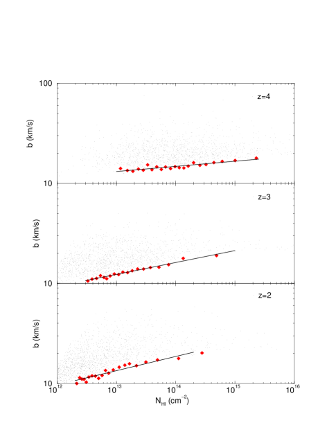
Figure 1: The column density-width ($N_{\rm HI}-b$) distribution at three redshifts ($z=4,3,2$) for our LCDM model with $\sigma_{8}=1.0$ and our standard heating rates. The points are about 1200 simulated lines, the filled diamonds trace the minimum in the $N_{\rm HI}-b$ distribution as described in the text, while the solid line is a fit to these points.

The sharp edge that defines the cutoff is fairly obvious to the human eye and has been previously noticed in both observations (e.g. [Kirkman & Tytler 1997]) and simulations ([Zhang et al. 1997]). In order to be more quantitative about the position of the cutoff, we take as our inspiration edge-detection techniques from machine-vision research. An edge — in one dimension — is defined as a zero in the second derivative of the intensity (since this is an extrema in the first derivative, the rationale is obvious). The application of this idea is quite straightforward.

First, we sort the lines by column density and divide them into groups of size 30-50 (each group is equivalent to a scan line in an image). The smoothed density of lines is then computed as a function of $b$ with a weighted sum over all lines in each group:

$$\rho_{b}(b)=\sum_{i}\exp(-(b_{i}-b)^{2}/2\sigma_{b}^{2}),$$ (22)

where $\sigma_{b}=3$ km/s is the smoothing constant. The method is not sensitive to small changes in either this parameter or to the number of points in the group (more lines per group mean less noise but lower resolution along the $N_{\rm HI}$ direction). We can compute derivatives of $\rho_{b}$ very easily, so we simply define, for each group with average column density $N_{HI,min}$, the edge to be at $b_{min}$ such that

$$\frac{d^{2}\rho_{b}}{db^{2}}(b_{min})=0.$$ (23)

For noisy data there are occasionally several zero crossings — we take the strongest, defined as the one with the largest first derivative. In order to get the lower cutoff, we insist that the first derivative be position. Software to perform this is available from the authors on request.

One important advantage of this algorithm is that it is relatively insensitive to noise which tends to smear out the data (but not shift the edge) or outliers in the $N_{\rm HI}-b$ distribution (which may be rogue metal lines or simply the result of blending). It also non-parametric in that it doesn’t assume a form for the $N_{\rm HI}-b$ line.

This results in a set of points which define the $N_{\rm HI}-b$ minimum and are plotted in Figure 1 as solid diamonds. We also show a least-squares power-law fit to the line. We used only absorption lines within a range of column densities which was selected to include the majority of lines but not go below about $2\times 10^{12}$ cm^-2 or above a few times $10^{15}$ cm^-2. The lower limit is slightly below present day observational limits and the upper limit marks the point were line dynamics becomes more complicated (i.e. affected by shocks and, in the real world, star formation).

Each of these points may be converted into a measurement of $T$ and $\delta_{b}$ via equations (9) and (2.1). The results are plotted in Figure 2 as open circles. Also shown is a measure of the temperature-density relation in the simulation by plotting 10000 random cells as dots. The solid line comes from converting the power-law fits from Figure 1 into measurements of $T_{0}$ and $\gamma$ via equation (12).

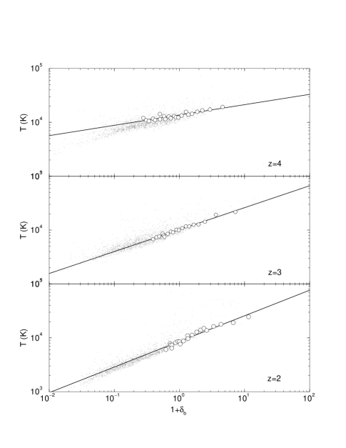
Figure 2: The temperature-overdensity relation for the same canonical LCDM model ($\sigma_{8}=1.0$) in Figure 1, shown at three redshifts: $z=4,3$ and 2. The dots are 10000 random cells, while the open circles and solid line are derived from the minimum $N_{\rm HI}-b$ line as described in the text.

The match is quite good, although clearly we preferentially probe the upper part of the $T-\delta$ relation. This is because, to be observed, a line must be more dense than the surrounding gas, so the measure is insensitive to the temperature of gas between filaments and sheets (although note that we can still probe densities significantly lower than the cosmic mean). On the other end, the maximum overdensity is around 10 because of the maximum $N_{\rm HI}$ limit. If the $T-\delta$ relation is not a strict power-law, as at $z=4$, then this can result in a substantial under- or over-estimate of the temperature at very low or very high densities. We also note that there are a small fraction of points in the simulation with moderate densities but very high temperatures. These points tend to lie near much more massive structures and have been enveloped in their accretion shock. The minimum $b$ method described here is not sensitive to these (rare) points.

We should remind the reader of two points about the normalization of the $\delta_{b}-N_{\rm HI}$ relation, equation (12). First, the normalization was selected to give a good match at $z=3$ — changing this value is roughly equivalent to shifting the open circles horizontally (in $1+\delta_{b}$). Second, the parameter $F$ shows there is a degeneracy amoung the parameters $\Omega_{b}$, $h$ and $\Gamma_{\rm HI}$ such that as long as the value of $F$ is unchanged, these parameters can be changed without affecting the results plotted here. In fact, this is one reason we choose to plot $1+\delta_{b}$ rather than a physical density. Although the individual parameters $\Omega_{b}$, $h$ and $\Gamma_{\rm HI}$ are not well determined, this particular combination is, from observations of the Ly$\alpha$ forest (see, for example, [Rauch et al. 1997]).

4.2 Changing the equation of state

Given our success in measuring the temperature of the IGM in the canonical simulation described in the previous section, it is interesting to see if we can detect the effect of changing the primary heating mechanism as outlined in the introduction. In this section, we show that this is possible. We retain the same cosmological model, but modify the HeII photo-heating rate as described in Abel & Haehnelt (1999)abe99. This takes into account radiative transfer effects during HeII photo-ionization that are neglected in these simulations. Since the amplitude of the effect is hard to gauge, we either multiply the rate by two or four.

The results are shown in Figure 3, again with $b_{min}$ points and fit as determined from our edge-detection algorithm. Here, in order to give a concrete comparison with observations and to provide a constant reference point, we also plot the observational equivalent of the $N_{\rm HI}-b$ minimum as found by Kirkman & Tytler (1997)kir97 at a mean redshift of 2.7 for a single line-of-sight. Although they fit this by eye the result agrees very well with the method used here. Our standard HeII photo-heating rate produces temperatures which are too low, while the x2 and x4 simulations are much closer and bracket the result, with the x2 case the closest. There is some evidence that the slope is in disagreement for all cases; however, this does not appear to be strongly significant given our level of uncertainty (see below). We can apply the same method used earlier to determine the $T-\delta$ relation, which is shown in the three left panels of Figure 4. Again, the equation of state is quite accurately determined.

Figure 3: The column density-width ($N_{\rm HI}-b$) distribution at $z=2.7$ for our canonical LCDM model with four different heating rates. The top frame shows the usual Haardt & Madau (1996) HeII photo-heating rate, while the next two panels demonstrate the effect of increasing this rate by factors of two and four, respectively. The bottom panel has the usual HeII rate but includes Compton X-ray heating. The filled diamonds describe the minimum in the $N_{\rm HI}-b$ distribution as described in the text. The solid line is a fit to these points, and the dashed line is the same for each panel and shows the observational determination of the $N_{\rm HI}-b$ minimum from Kirkman & Tytler (1997).

Next, we examine the importance of Compton X-ray heating in the bottom panel of Figure 3, which is again our canonical LCDM simulation with the usual HeII photo-heating rates. However, now we include hard X-ray heating as described earlier. While this does boost the temperature somewhat, it is clearly — by itself — insufficient to match observations. Since the Compton heating rate is independent of density, it tends to flatten the temperature-density relation, shown in the upper right panel of Figure 4. However, the effect at $z=2.7$ is mostly limited to low densities and so is very difficult to detect with the minimum $N_{\rm HI}-b$ method.

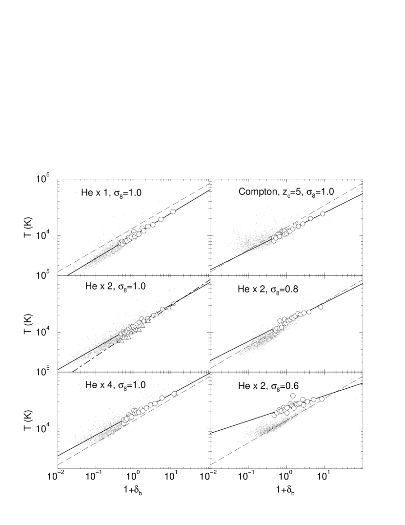
Figure 4: The temperature-overdensity relation at $z=2.7$ for six simulations. The symbols are as in Figure 2. The three left panels are from the canonical LCDM model (with $\sigma_{8}=1.0$) for the same three values of HeII photo-heating rate as in Figure 3. The upper right panel is for the same model but with X-ray Compton heating instead. The two lower panels on the right were run with twice the usual Haardt & Madau HeII photo-heating rate but for low-power LCDM models, with $\sigma_{8}=0.8$ and $\sigma_{8}=0.6$. For comparison, each plot also shows the equation of state from the middle left frame as a dashed line. The triangles and dot-dashed line in the middle-left panel show the equation of state derived from a different Voigt-profile fitting technique as described in the text.

4.3 Changing the power spectrum

Although we have been successful in measuring the equation of state for our canonical LCDM model, we argued in section 2 that the amplitude of fluctuations on scales of a few hundred kpc is also important in determining the distribution of line widths. In this section, we will demonstrate that for some models, this effect prevents us from accurately measuring the temperature-density relation.

Figure 5 shows the results from two LCDM models in which the power has been reduced to $\sigma_{8}=0.8$ and $\sigma_{8}=0.6$. This changes the derived minimum $N_{\rm HI}-b$ line. For $\sigma_{8}=0.8$ (the top panel) the match with observations is very good, while the lower power simulation produces a power-law fit that is too flat. Since the equation of state has not changed, application of the $N_{\rm HI}-b$ minimum method results in temperatures which are too hot, particularly for the lowest-power run. This shown in the bottom right panels of Figure 4.

Figure 5: The column density-width distribution ($N_{\rm HI}-b$) at $z=2.7$ for two LCDM simulations. These both use twice the usual HeII heating rate, but decrease the amplitude of the initial fluctuation spectrum to $\sigma_{8}=0.8$ (top) and $\sigma_{8}=0.6$ (bottom). The symbols are as in Figure 3.

This happens because one of our key assumptions is violated: specifically that there be a substantial number of lines for which $b_{vel}$ be small. For the lower-power models, the smallest filaments are almost all in the pre-turnaround stage. That is, their peculiar velocities are still smaller than the Hubble flow across their width, so that these two values cannot cancel. This preferentially affects low column density lines because they are the smallest fluctuations. In fact, lines with a column density of around $N_{\rm HI}\sim 10^{15}$ cm^-2 ($1+\delta_{b}\sim 10$) faithfully reproduce the correct temperature even for the $\sigma_{8}=0.6$ simulation.

This demonstrates that the minimum $N_{\rm HI}-b$ method suffers from a degeneracy between the gas temperature and the amplitude of fluctuations. As long as $\sigma_{34}\gtrsim 1.6$, the method can be used in a straightforward fashion (we use $\sigma_{34}$ since this is much closer to the scale and redshift of interest and so is nearly independent of other cosmological parameters). Below this value, there is still useful information to be gained, but the interpretation is more complicated. In particular, without other knowledge about $\sigma_{34}$, the value of $T_{0}$ derived in this way is an upper limit and the value of the slope $\gamma$ is a lower limit.

Although we do not show the results here, we have also analyzed an LCDM simulation with a lower value of the Hubble constant as well as an SCDM model (see Table 1). The results agree with the trends discussed in this section.

It is important to ask at this point what the uncertainties are in determining the minimum $N_{\rm HI}-b$ line. The primary source of uncertainty is fitting the Voigt-profiles in the first place, as this is both non-linear and non-unique (e.g. [Kirkman & Tytler 1997]). In order to gauge the magnitude of the possible error, we select one simulation (LCDM $\sigma_{8}=1.0$ with twice the usual HeII photo-ionizing rate) and fit it with the more realistic method AUTOVP ([Davé et al. 1997]), kindly provided by Romeel Davé. This method performs a chi-squared minimization to produce the line list from the simulated spectrum. Figure 6 shows the result for a signal-to-noise ratio of 60, along with the fit found with the more idealized Voigt-profile fitting algorithm. Clearly there is some difference, which also affects the derived equation of state, shown in the middle-left panel of Figure 4. This amounts to about a 15% difference in $T$ at $\delta_{b}=0$, and is mostly due to fitting Voigt-profiles to lines which do not follow this profile in detail.

Figure 6: The column density-width distribution ($N_{\rm HI}-b$) at $z=2.7$ for a LCDM simulation with $\sigma_{8}=1.0$ and twice the usual HeII photo-heating rate. This is the same simulation analyzed in the second panel of Figure 3, but here we use a different Voigt-profile fitting technique. The diamonds and solid line are the derived minimum $N_{\rm HI}-b$ line, while the dot-dashed line is the minimum $N_{\rm HI}-b$ fit found previously, for comparison.

5 The median of the $b$-distribution

We have so far focused on the low $b$ cutoff, but now turn, briefly, to the rest of the distribution. The top panel of Figure 7 shows $dn/db$ at $z=2.7$ for our three $\sigma_{8}=1.0$ models with varying equations of state (i.e. different HeII photo-heating rates). Only lines in the range $N_{\rm HI}=10^{13.1}-10^{14}$ cm^-2 are used so as not to be biased by the line-selection function. All distributions are normalized so that $\int(dn/db)db=1$. This plot shows that increasing the temperature results in a constant shift in $\log(b)$. As discussed in Bryan et al. (1999), this is not primarily a result of thermal Doppler broadening, but comes instead from a thickening of the filaments and sheets (in both physical and velocity space) due to the influence of the increased pressure — gas is driven out of the centers of the filaments.

Figure 7: The simulated $b$ distribution function for three models with the same power but different temperatures (top), the same temperature but differing power (middle) and all models scaled as described in the text(bottom).

The middle panel of Figure 7 shows the effect of changing the amplitude of the power spectrum while keeping the temperature constant. The results appear to match the simple scaling derived in section 2. This degeneracy between temperature and power can be written in terms of the median of this distribution:

$$b_{med}(T_{0}^{\prime},\sigma_{34})=26.5{\rm km/s}\left(\frac{T_{0}^{\prime}}{10000K}\right)^{1/2}\left(\sigma_{34}\right)^{-1/2}$$ (24)

We use $T_{0}^{\prime}$ to indicate the temperature at $\delta_{b}=0$ measured directly from the simulations, rather than via the minimum $N_{\rm HI}-b$ method. In Figure 8, we plot this function against the measured median $b$ parameters from our simulations. Finally, in order to demonstrate that there is not much change in the shape, we rescale the $b$ distributions in the top two panels of Figure 7 with the following transformation: $b\rightarrow fb$ and $(dn/db)\rightarrow(dn/db)/f$. We define $f=b_{med}(T_{0}^{\prime},\sigma_{34})/b_{med}(13000K,1.93)$, where $b_{med}$ is given in equation (24). The result is shown in the bottom panel of this figure. The scaling works very well, indicating that the shape of the distribution changes little, once the median is specified. The biggest differences are at small $b$, where thermal Doppler broadening dominates.

Figure 8: The median of the $b$ distribution depends almost entirely on just two parameters: the temperature of the gas ($T_{0}^{\prime}$) and the amplitude of the power spectrum ($\sigma_{34}$).

Our simulated boxes are too small to fully contain all the large-scale power. Previously ([Bryan et al. 1999]) we showed that this has little effect on the shape of the $b$ distribution but can cause a small shift in the median. In order to gauge the size of this effect here, we ran two models with $\sigma_{8}=0.8$, one with our usual box-length of 4.8 Mpc and one with twice this size (see Table 1). The both had the same cell size (i.e. the larger box simulation had $256^{3}$ cells rather than our more usual $128^{3}$). The change in the median was only 0.4 km/s (1.6%). This could be slightly larger for models with more power, but is unlikely to be a significant effect.

6 A preliminary comparison to observations

In this section, we make a preliminary comparison to observations, using previously published results from the quasar HS1946+7658 ([Kirkman & Tytler 1997]) at a mean redshift $<z>=2.7$ and APM 08279+5255 ([Ellison et al. 1999]) at $<z>=3.4$. Both observations have high signal-to-noise ratios, ranging from 15 to 100 for HS1946+7658 and 30 to 150 for APM 08279+5255. It should be kept in mind that the Voigt profile fitting technique used in these papers (which is not fully automated) differs somewhat from both methods used here. The $N_{\rm HI}-b$ distributions are shown in Figure 9, along with the derived minimums using our edge-detection method. (for APM 08279+5255 we adopt a minimum column density of $2\times 10^{13}$ cm^-2 due to concerns about line-blending at these high redshifts).

Figure 9: The column density-width distribution ($N_{\rm HI}-b$) at for two sets of observed absorption line systems. The top is HS 1946+7658 ([Kirkman & Tytler 1997]) at $<z>=2.7$ and the bottom is from APM 08279+5255 ([Ellison et al. 1999]) at $<z>=3.4$. The symbols are as in Figure 3.

The minimum $N_{\rm HI}-b$ edges detected can be converted into a measurement of the temperature-density relation, which is shown in Figure 10. The values of $F$ required to convert column density to $1+\delta_{b}$ were determined by fitting the column density distribution to the simulations (we use the LCDM $\sigma_{8}=0.8$ simulation but this is not very sensitive to which model we select). The noise in the $T-\delta_{b}$ relation is larger than for the simulations because of the much smaller number of lines ($\sim 300$ as compared to $\sim 1200$). The power law fits are given by $T_{0,4}=1.65$, $\gamma=1.29$ (HS1946+7658) and $T_{0,4}=1.52$, $\gamma=1.54$ (APM 08279+5255). We remind that reader that these determinations are really upper limits to the temperature rather than measurements because of the possible effects of cosmology (i.e. the unknown value of $\sigma_{34}$).

There is an indication from the higher-redshift system that the gas is cooler at low density (i.e. a steeper equation of state), although clearly this is substantialy uncertainty. Still, a similar trend of lower $b$ lines at higher redshift has been previously noted from different data ([Hu et al. 1995]; [Kim et al. 1997]), so it is worth considering the possibility that (low density) gas is cooler at higher redshift. This does not agree with what is expected for gas dominated by steady photo-ionization heating and adiabatic cooling: $T_{0}\sim(1+z)^{1.7}$ with a slowly steepening equation of state slope ([Meiksin & Madau 1993]; [Miralda-Escudé & Rees 1994]; [Hui & Gnedin 1997]; [Abel & Haehnelt 1999]). An alternate heating source, such as late Helium reionization, would be required if this result proves true.

Figure 10: The temperature-density relation as derived from the two quasars analyzed in Figure 9.

To compare the shape of the $b$ distributions to observations, in Figure 11 we plot $dn/db$ from the same two quasar systems previously discussed. We also show the distribution from our LCDM $\sigma_{8}=0.8$ simulation with twice the Haardt & Madau HeII photo-heating rate. The shape is in reasonable agreement with HS1946+7658, but the other system has a large number of very low $b$ lines which are not seen in any of the models considered here (although a very low temperature model might match). Both observed systems also have a more pronounced non-Gaussian tail at large $b$ than appears in the simulations. Note, however, that the log-log plot accentuates this tail when compared to the more usual linear plot. It should also be kept in mind that the Voigt-profile fitting method used for the observations differs from either employed in this paper. Clearly, a more definitive result will require identical treatment of data and simulations. The bottom panel of the same Figure shows how the two different Voigt-profile fitting algorithms used in this work compare.

Figure 11: Top: $b$ distributions from two observed quasar line systems along with one of the better fitting simulated results; bottom: $dn/db$ for the same simulation using two different Voigt-profile fitting algorithms: the solid line shows ZANM97 ([Zhang et al. 1998]) which is quite idealized, while the dashed line indicates AUTOVP ([Davé et al. 1997]) which includes random noise with a signal-to-noise ratio of 60.

The observed median $b$ (in the same column density range considered earlier) is 27.3 for both systems. Using equation (24), this implies that

$$\left({T_{0}^{\prime}}/{10000K}\right)^{1/2}\left(\sigma_{34}\right)^{-1/2}=1.03.$$ (25)

If we use the upper limits for $T_{0}$ derived earlier from the $N_{\rm HI}-b$ distribution, then we can get an upper limit on the amplitude of the power spectrum: $\sigma_{34}\lesssim 1.52$. The uncertainty is about 20%, due to the uncertainty in the measured temperature. This is quite close to the minimum value of $\sigma_{34}$ required for a straightforward interpretation of the $N_{\rm HI}-b$ minimum method ($\sigma_{34}\gtrsim 1.6$). Interestingly, this value of $\sigma_{34}$ (around 1.5-1.6) agrees well with a number of determinations of the power spectrum amplitude using other characteristics of the Ly$\alpha$ forest ([Gnedin 1998]; [Croft et al. 1999]). For the LCDM model it is also in accordance with the normalization from COBE and rich clusters of galaxies (e.g. [Liddle et al. 1996]).

7 Conclusions

In this paper, we have investigated a method for determining the relation between density and temperature (loosely denoted the equation of state of the IGM) from the distribution of quasar absorption lines in the $N_{\rm HI}-b$ plane. Specifically, we look for a sharp minimum line in this plane arising from the fact that Doppler thermal broadening sets a minimum line width. Because there is a tight relation between column density and overdensity, we can relate $N_{\rm HI}$ to overdensity and $b$ to temperature. We derive a simple model which reproduces this behaviour, and state clearly its assumptions.

We test this method with a range of equations of state, including an enhanced HeII photo-heating rate (assumed to be due to neglected optical transfer effects) and X-ray Compton heating. We show that the method works as long as the power spectrum amplitude is sufficiently high, so that $\sigma_{34}\gtrsim 1.6$. If the density fluctuations are too small, then one important assumption fails: that there be a substantial fraction of lines whose width is dominated by thermal broadening. When this occurs, it mimics an equation of state which is hotter and flatter.

Very recently, Schaye et al. (1999)sch99 independently investigated the feasibility of using this method. They used a different method for identifying the $N_{\rm HI}-b$ cutoff, but came to quite similar conclusions as presented here, with one important exception. They argued that there was no cosmological dependence on the cutoff in the $N_{\rm HI}-b$ plane, in disagreement with the results in this paper. However, they examined a relatively small number of simulations which all had similar values of $\sigma_{34}$, mostly comparable to, or somewhat larger than, the critical value listed above. In this case, it would be very difficult to notice the effect due to power.

Applying our results to two quasar lines-of-sight with mean redshifts of $z=2.7$ and $z=3.4$, we derive a temperature-density relation from these two systems that is similar to those found in at least some of the simulations presented here. We find a temperature of approximately $16000$ K for gas with the mean density rising to about $35000$ K for an overdensity of six. The uncertainty of these numbers is around 20%, however without any more information about the value of $\sigma_{34}$, they must be treated as upper limits to the temperature of the gas. If we were to assume that the power spectrum criterion is satisfied then this represents fairly hot gas compared to traditional models. The additional HeII photo-heating is sufficient to produce this much heat; however, by itself Compton X-ray heating is not.

We turn now from the $N_{\rm HI}-b$ minimum to $dn/db$, the distribution of $b$ parameters. Following similar earlier work ([Hui & Rutledge 1999]), we present a simple linear argument which shows that the other important parameter in determining the $b$ parameter distribution is the amplitude of the power spectrum. We demonstrate that simulations reproduce this scaling ($b_{med}\sim T^{1/2}\sigma_{34}^{-1/2}$), and show that the shape of the $b$ distribution stays nearly invariant to changes in temperature or the power spectrum amplitude. Its median value can be given as a simple function of the gas temperature and $\sigma_{34}$ (at $z\sim 3$). If we use the temperature derived from the $N_{\rm HI}-b$ method, this implies that $\sigma_{34}\sim 1.5$ (with an uncertainty of about 20%), a value which is in reasonable agreement with other methods of determining the amplitude of the power spectrum. It should be kept in mind that since the temperature measurement is really an upper limit, then this value for $\sigma_{34}$ is also an upper limit.

Theuns et al. (1999)the99 also investigated the cosmological dependence of the $b$-distribution. They found the results sensitive to the gas temperature (as we have here), but did not find the sensitivity to power spectrum discussed here. Again, it seems likely that this is due to the small range in spectral amplitudes of their simulations.

The degeneracy described in this paper between power and temperature means that the $b$ distribution alone will not be sufficient to determine the equation of state of the gas. This is unfortunate because the evolution of the temperature-density relationship can provide constraints on other cosmological interesting events. For example, if the gas were to be colder above $z=3$ (as the data presented here might be indicating), one possible explanation would be the late reionization of helium ([Reimers et al. 1997]; [Haehnelt & Steinmetz 1998]; [Abel & Haehnelt 1999]). This degeneracy can be broken by using other aspects of the Ly$\alpha$ forest (e.g. [Croft et al. 1998]; [Machacek et al. 1999]) to independently fix the amplitude of fluctuations at these scales and redshifts.

We acknowledge useful discussion with Tom Abel, Piero Madau, Avery Meiksin and Lam Hui. Some of data presented herein were obtained at the W.M. Keck Observatory, which is operated as a scientific partnership amoung the California Institute of Technology, the University of California and the National Aeronautics and Space Administration. The Observatory was made possible by the generous financial support of the W.M. Keck Foundation. This work is done under the auspices of the Grand Challenge Cosmology Consortium and supported in part by NSF grants ASC-9318185 and NASA Astrophysics Theory Program grant NAG5-3923. Support for this work was also provided by NASA through Hubble Fellowship grant HF-01104.01-98A from the Space Telescope Science Institute, which is operated by the Association of Universities for Research in Astronomy, Inc., under NASA contract NAS6-26555.

References

- [Abel & Haehnelt 1999] Abel, T. & Haehnelt, M.G. 1999, preprint (astro-ph/9903102)
- [Anninos et al. 1997] Anninos, P., Zhang Y., Abel, T., Norman, M.L., 1997, New Astronomy, 2, 209
- [Bi, Börner & Chu 1992] Bi, H., Börner, G. & Chu, Y. 1992, A&A, 266, 1
- [Bond, Szalay & Silk 1988] Bond, J.R., Szalay, A.S. & Silk, J. 1988, ApJ, 324, 627
- [Bryan et al. 1995] Bryan, G.L., Norman, M.L., Stone, J.M., Cen, R., Ostriker, J.P. 1995, Comput. Phys. Comm., 89, 149
- [Bryan et al. 1999] Bryan, G.L., Machacek, M., Anninos, P. & Norman, M.L., ApJ, 514, 13
- [Cen et al. 1994] Cen, R., Miralda-Escudé, J., Ostriker, J.P., Rauch, M. 1994, ApJ, 437, L9
- [Croft et al. 1998] Croft, R.A.C., Weinberg, D.H., Katz, N., Hernquist, L. 1998, ApJ, 495, 44
- [Croft et al. 1999] Croft, R.A.C., Weinberg, D.H., Pettini, M., Hernquist, L. & Katz, N. 1999, ApJ, in press
- [Croft, Hu & Davé 1999] Croft, R.A.C., Hu, W., & Davé, R. 1999, submitted to Phys. Rev. Lett.
- [Davé et al. 1997] Davé, R., Hernquist, L., Weinberg, D.H. Katz, N. 1997, ApJ, 477, 21
- [Doroshkevich & Shandarin 1977] Doroshkevich, A.G. & Shandarin, S. 1977, MNRAS, 179, 95
- [Eisenstein & Hu 1999] Eisenstein, D.J. & Hu, W. 1999, ApJ, 511, 5
- [Ellison et al. 1999] Ellison, S.L., Lewis, G.F., Pettini, M., Sargent, W.L., Chaffee, F.H., Foltz, C.B., Rauch, M., Irwin, M.J. 1999, PASP, in press
- [Gnedin 1998] Gnedin, N.Y. 1998, MNRAS, 299, 392
- [Gnedin & Hui 1998] Gnedin, N.Y. & Hui, L.. 1998, MNRAS, 296, 44
- [Haardt & Madau 1996] Haardt, F. & Madau, P. 1996, ApJ, 461, 20
- [Haehnelt & Steinmetz 1998] Haehnelt, M.G. & Steinmetz, M. 1998, MNRAS, 298, 21L
- [Hernquist et al. 1996] Hernquist, L., Katz, N., Weinberg, D.H., Miralda-Escudé, J. 1996, ApJ, 457, 51L
- [Hui, Gnedin & Zhang 1997] Hui, L., Gnedin, N.Y. & Zhang, Y. 1997, ApJ, 486, 599
- [Hui & Gnedin 1997] Hui, L. & Gnedin, N.Y. 1997, MNRAS, 292, 27
- [Hui & Rutledge 1999] Hui, L. & Rutledge, R.E. 1999, ApJ, 517, 541
- [Hu et al. 1995] Hu, E., Kim, T.-S., Cowie, L.L., Songaila, A., & Rauch, M. 1995, AJ, 110, 1526
- [Kim et al. 1997] Kim, T.-S., Hu, E.M., Cowie, L.L. & Songaila, A. 1997, AJ, 114, 1
- [Kirkman & Tytler 1997] Kirkman, D. & Tytler, D. 1997, ApJ, 484, 672
- [Machacek et al. 1999] Machacek, M., Bryan G.L., Meiksin, A., Anninos, P., Thayer, D., Norman M. & Zhang, Y. 1999, ApJ, submitted
- [Madau & Efstathiou 1999] Madau, P. & Efstathiou, G. 1999, preprint (astro-ph/9902080)
- [McGill 1990] McGill, C. 1990, MNRAS, 242, 544
- [Meiksin & Madau 1993] Meiksin, A. & Madau, P. 1993, ApJ, 412, 34
- [Miralda-Escudé & Rees 1994] Miralda-Escudé, J. & Rees, M.J. 1994, MNRAS, 266, 343
- [Nath, Sethi & Shchekinov 1999] Nath, B.B., Sethi, S.K. & Shchekinov, Y. 1999, MNRAS, 303, 1
- [Nusser & Haehnelt 1999] Nusser, A. & Hauhnelt, M. 1999, MNRAS, 303, 685.
- [Peebles 1993] Peebles, P.J.E., Principles of Physical Cosmology, Princeton: Princeton University Press
- [Petitjean, Müket & Kates] Petitjean, P. Müket, J.P., & Kates, R.E. 1995, A&A, 295, L9
- [Rauch et al. 1997] Rauch, M., Miralda-Escudé, J., Sargent, W.L.W., Barlow, T.A., Weinberg, D.H., Hernquist, L., Katz, N., Cen, R., Ostriker, J.P. 1997, ApJ, 489, 7
- [Rees 1986] Rees, M. 1986, MNRAS, 218, 25P
- [Reimers et al. 1997] Reimers, D., Köhler, S., Wisotzki, L., Groote, D., Rodriguez-Pascal, P., Wamsteker W., 1997, A&A, 327, 890
- [Schaye et al. 1999] Schaye, J. Thuens, T., Leonard, A. & Efstathiou, G. 1999, MNRAS, in press
- [Theuns et al. 1998] Theuns, T., Leonard, A., Efstahtiou, G., Pearce, F.R., & Thomas, P.A. 1998, MNRAS, 297, L49
- [Theuns et al. 1999] Theuns, T., Leonard, A., Schaye, J., & Efstahtiou, G. 1999, MNRAS, in press
- [Liddle et al. 1996] Liddle, A.R., Lyth, D.H., Viana, P.T.P., White, M. 1996, MNRAS, 282, 281L
- [Zhang et al. 1995] Zhang, Y., Anninos, P., Norman, M.L. 1995, ApJ, 453, L57
- [Zhang et al. 1997] Zhang, Y., Anninos, P., Norman, M.L., Meiksin, A. 1997, ApJ, 485, 496
- [Zhang et al. 1998] Zhang, Y., Meiksin, A., Anninos, P., Norman, M.L. 1998, ApJ, 495, 63