Constraining the History of the Sagittarius Dwarf Galaxy Using Observations of its Tidal Debris

Abstract

We present a comparison of semi-analytic models of the phase-space structure of tidal debris with measurements of average distances, velocities and surface densities of stars associated with the Sagittarius dwarf galaxy (Sgr), compiled from all observations reported since its discovery in 1994.

We find that several interesting features in the data can be explained by these models. The properties of stars $\sim\pm 10-15^{o}$ away from the center of Sgr — in particular, the orientation of material perpendicular to Sgr’s orbit (Alard 1996, Mateo et al 1996, Fahlman et al 1996, Alcock et al 1997) and the kink in the velocity gradient (Ibata et al 1997) — are consistent with those expected for unbound material stripped during the most recent pericentric passage $\sim 50$Myrs ago. The break in the slope of the surface density seen by Mateo, Olszewski & Morrison (1998) at $b\sim-35^{o}$ can be understood as marking the end of this material. However, the detections beyond this point are unlikely to represent debris in a trailing streamer, torn from Sgr during the immediately preceding passage $\sim 0.7$Gyrs ago, as the surface-density of this streamer would be too low compared to observations in these regions. The low $b$ detections are more plausibly explained by a leading streamer of material that was lost more that 1 Gyr ago and has wrapped all the way around the Galaxy to intercept the line of sight. The distance and velocity measurements at $b=-40^{o}$ reported in Majewski et al (1999) also support this hypothesis.

We determine debris models with these properties on orbits that are consistent with the currently known positions and velocities of Sgr in Galactic potentials with halo components that have circular velocities $v_{\rm circ}=140-200$ km/s. In all cases, the orbits oscillate between $\sim$12 kpc and $\sim$40 kpc from the Galactic center with radial time periods of $0.55-0.75$Gyrs. The best match to the data is obtained in models where Sgr currently has a mass of $\sim 10^{9}M_{\odot}$ and has orbited the Galaxy for at least the last 1 Gyr, during which time it has reduced its mass by a factor of 2-3, or luminosity by an amount equivalent to $\sim 10\%$ of the total luminosity of the Galactic halo. These numbers suggest that Sgr is rapidly disrupting and unlikely to survive beyond a few more pericentric passages. These conclusions are only tentative because they rely heavily on the less-certain measurements of debris properties far from the center of Sgr. However, they demonstrate the immense potential for using debris to determine Sgr’s dynamical history in great detail.

1 Introduction

Since its discovery in 1994 (Ibata, Gilmore & Irwin 1994, 1995 — hereafter I (94) and I (95)), the history of the Sagittarius dwarf galaxy (Sgr) has been a matter of some debate. Sgr is centered on the globular cluster M54 at $(l,b)=(6^{o},-14^{o})$ on the opposite side of the bulge from us at 16 kpc from the Galactic center and is apparently moving towards the Galactic plane (I (94, 95), Ibata et al 1997 — hereafter I (97)). The isopleths revealed by careful star count analyses (I (94, 95, 97)) are highly elongated along the direction of its motion, and populations plausibly associated with it have been found even further upstream and downstream (see Alard 1996, Mateo et al 1996, Fahlman et al 1996, Alcock et al 1997, Mateo, Olszewski & Morrison 1998 and Majewski et al 1999 — hereafter A (96); M (96); F (96); A (97); M (98) and Paper I respectively). In addition, Irwin & Totten (1999) have found an excess in the surface density of carbon stars aligned with the direction of elongation of Sgr that completely encircles the Galaxy. This suggests that Sgr is being strongly influenced by the Milky Way’s tidal field, possibly completely destroyed, yet its proximity to the Galactic center also indicates that it may have had time to circle the Galaxy many times. If we are currently witnessing just one in a long series of encounters it seems unlikely that it should also be the last.

Johnston, Spergel & Hernquist (1995) tackled this problem using $N$-body simulations to investigate the evolution of stellar systems along highly eccentric orbits that would suffer few encounters during the lifetime of the Galaxy. They found that they could fit nearly all the observations available at that time with a wide variety of models, without requiring that this be either the first or last passage of Sgr. However, they did not attempt to fit the lack of velocity gradient reported in the center of Sgr (I (95)). Velásquez & White (1995) demonstrated that this datum alone suggests that Sgr cannot be on a highly eccentric orbit, and their estimate for the proper motion of Sgr has since been confirmed by observations (I (97)), and rules out the specific models investigated by Johnston, Spergel & Hernquist (1995). I (97) argue that if Sgr is embedded in a dark matter halo, it could in fact be impervious to tidal destruction, but concede that it could be being stripped and limited by the Galactic tidal field. This idea is illustrated with numerical simulations by Ibata & Lewis (1998). Finally, Zhao (1998) suggests that the proper motion measurements of Sgr and the Large Magellanic Cloud (LMC) are consistent with a scenario in which Sgr was initially on an orbit much farther from the Galactic center – and hence immune to the affect of the Galactic tidal field – and has only recently been flung into it’s current orbit through a collision with the LMC.

If we could measure how fast Sgr is currently losing mass, and constrain how much mass it has lost in the past, we could make some progress towards resolving this debate about its history and current state. In this paper we address these questions by building semi-analytic models of the structure of tidal debris that are consistent with all the current position- and velocity-space observations of material believed to be associated with Sgr. In §2.1 we describe sources and characteristics of the data used to constrain the models and in §2.2 we outline the method for building the semi-analytic models. We present models which agree with all the observations in §3 and discuss the extent of the limitations that the data places on Sgr’s orbit, current mass and mass loss history, and the potential of the Milky Way. We summarize our results in §4.

2 Tools

2.1 Summary of Data Sets

In this study we have combined data from eight different investigations that are currently available in the literature. We take the distance (24 kpc), line-of-sight velocity (170 km/s) and proper motion from I (94, 95) and I (97), and the velocity trends along the major axis of Sgr from Table 3 of I (97). At $b=-7^{o}$ and $b=-4^{o}$ ($+7^{o}$ and $+10^{o}$ away from the center of Sgr towards the Galactic disk) we have two more distance estimates from the discovery of associated RR Lyraes (A (96, 97)), and at $b=-23^{o}$ we have distances both from RR Lyraes (M (96)) and main-sequence fitting (F (96)) to Sgr populations found serendipitously in studies of the globular cluster M55. We also have one distance and a tentative velocity measurement at $b=-40^{o}$ (see Paper I for discussion). Finally, we use the surface density profile reported in M (98), which was produced from star counts at the position of the Sgr upper-main sequence in a set of 24 color-magnitude diagrams that cover the expected locus of Sgr’s debris trail sky from $b=-24^{o}$ to $b=-48^{o}$.

The symbols in Figure 1 summarize this combined data set, with the solid line in Panels (a), (b) and (c) showing the locus of an orbit calculated from the position and velocity of Sgr and the meaning of the symbols in each panel summarized in Panel (c). Panel (a) shows the position of Sgr projected onto the plane containing the Sun (at $(X,Z)=(-8,0)$kpc in this coordinate system) and perpendicular to the Galactic disk. Panels (b), (c) and (d) show the distance from the Sun, line-of-sight velocity in a Galactic frame of rest and (arbitrarily normalized) surface density measurements plotted against Galactic latitude. (Note: the surface density of stars identified as possibly belonging to Sgr in Paper I agrees with M (98)’s estimate and this point is also included in Panel (d) for comparison.)

When we allowed Sgr’s proper motion to vary within the quoted error bars (I (97)) and compared the different data sets both with each other and with the loci of the orbits we found a number of interesting features, already noted by previous authors: the distances in the central regions of Sgr follow a line perpendicular to the orbit rather than aligned with it; there is a kink in the velocities measured by I (97) that is hard to reconcile with the orbit calculations alone; although the distance measurement at $b=-40^{o}$ from Paper I typically lies close to the orbit, the velocity measurement does not; and there is a break in the slope of the Sgr star counts at $b=-35^{o}$. In §3 we will demonstrate how all these features could be a natural consequence of debris dispersal from the disruption of Sgr.

2.2 Summary of Method

In this section we briefly outline the semi-analytic method we employ to model debris dispersal — the details are reported in Johnston (1998a, 1998b). The method predicts the full phase-space positions and densities of mass lost at a given time from a satellite of known mass, $m_{\rm sat}$, and motion orbiting in a specified parent galaxy potential, $\Phi$, at any later time.

When a satellite disrupts, escaping stars that lose (gain) energy move ahead of (behind) the satellite to form leading (trailing) streams of debris along its orbit. In a given parent galaxy potential $\Phi$, the gain or loss of energy $\Delta E$ of a star can be related to its position at any time following the mass loss event by comparing the time period of a circular orbit of energy $E+\Delta E$ with that of the unperturbed satellite orbit of energy $E$ (ignoring the weak dependence of orbital periods on angular momentum), and adjusting the azimuthal position of debris along the orbit accordingly. The star’s $\Delta E$ also gives an estimate of its offset in distance from the orbit: $\Delta R\sim\Delta E/(d\Phi/dR)$. The semi-analytic method combines this approximate modeling of particle dynamics with (1) an analytic description of the energy scale $\epsilon=R(m_{\rm sat}/M_{Gal})^{1/3}d\Phi/dR$ (where $M_{Gal}$ is the mass of the parent galaxy enclosed within radius $R$) in tidal debris; (2) the intrinsic energy distribution (in scaled energy units $\Delta E/\epsilon$) observed in $N$-body simulations of satellite disruption. The method is further simplified by the observation that in simulations of satellite destruction most mass loss occurs near the pericenter of the satellite’s orbit and hence its mass loss history can be approximated as a series of discrete mass loss events. Despite these simplifications, the semi-analytic method successfully reproduces the density, position and velocity of streamers in a wide variety of simulations (for a given satellite mass, orbit and approximate mass-loss history) at a tiny fraction of the simulation’s computational cost (Johnston 1998a, 1998b). This makes the method an ideal tool for interpreting observations such as those described above because it allows a quick and thorough exploration of parameter space.

Several limitations should be noted. First, the method does not take into account the effect of dynamical friction on the orbit of the satellite. From Binney & Tremaine (1987) equation 7-27, the dynamical friction timescale for a $10^{9}M_{\odot}$ satellite orbiting at $R=$15 kpc from the center of the Galaxy is $\sim 5$ Gyrs. Since we consider $\leq 1.5$ Gyrs in the evolution of satellites of mass $\leq 10^{9}M_{\odot}$ on orbits where most time is spent at $R>15$ kpc, we expect this simplification to be unimportant. Moreover, our interpretation of the data is only intended to be approximate. However, once our knowledge of the structure and extent of debris associated with Sgr becomes detailed enough to warrant a more specific interpretation of its history, the effect of dynamical friction should be included.

Second, the method is most accurate for small satellites, with masses such that $(m_{\rm sat}/M_{Gal})^{1/3}\ll 1$ — for our own Galaxy this suggests it should only be used to study satellites, such as Sgr, with $m_{\rm sat}\leq 10^{9}M_{\odot}$. Finally, the method was developed and tested under circumstances where the satellite’s orbit was eccentric but not radial, and where the satellite’s structure was supported by random motions. Sgr satisfies both these conditions.

3 Results

3.1 General Approach

Our aim is to explore whether the combined data sets are consistent with the semi-analytic models of debris dispersal from satellite disruption and how much such a model can tell us about Sgr’s history, orbit and the Milky Way’s potential. We do not attempt to use an automated routine to find the “best fit” model since we believe that neither the extent of the data nor the accuracy of the models at present justify this level of sophistication. We instead simply compare the data and the models by visual inspection, varying four parameters:

1. $f$ — the fraction of mass lost on each pericentric passage. We assume that mass loss occurs instantaneously at pericenter and that $f$ is constant (as is approximately true in simulations).

2. $m_{\rm Sgr}$ — the mass of material still bound to Sgr and centered around M54.

3. $v_{\rm t}$ — Sgr’s velocity transverse to the line of sight. We take Sgr’s orbit to be exactly polar, fix its line-of-sight velocity to its observed value (170 km/s), and allow $v_{\rm t}$ to vary within the error-bars on the proper motion measurement quoted in I97. In fact, Sgr’s motion parallel to the Galactic plane is poorly constrained by current observations (I (97)), although the surface density contours do indicate that it must be on a near-polar orbit, and hence it is likely to be small. We will discuss the effect of non-polar orbits in flattened halo potentials in §3.5.

4. $v_{\rm circ}$ — the circular velocity of the dark matter halo, as defined in equation (3) below. We integrate Sgr’s orbit in Milky Way potentials of the form $\Phi=\Phi_{\rm bulge}+\Phi_{\rm disk}+\Phi_{\rm halo}$ where

   $$\Phi_{{\rm bulge}} = -{{GM_{{\rm bulge}}}\over{\sqrt{R^{2}+z^{2}}+c}},$$ (1)

   $$\Phi_{{\rm disk}} = -{{GM_{{\rm disk}}}\over{\sqrt{R^{2}+(a+\sqrt{z^{2}+b^{2}})^{2}}}},$$ (2)

   $$\Phi_{{\rm halo}} = {\frac{v_{{\rm circ}}^{2}}{2}}\ln(R^{2}+z^{2}/q^{2}+d^{2}).$$ (3)

   Here $R$ and $z$ are cylindrical coordinates aligned with the Galactic disk and the numerical values adopted for the parameters are $M_{{\rm disk}}=1.0\times 10^{11},M_{{\rm bulge}}=3.4\times 10^{10},a=6.5,b=0.26,c=0.7$ and $d=12.0$, where masses are in $M_{\odot}$, velocities are in km/s and lengths are in kpc. We vary $v_{\rm circ}$ between 140 km/s and 200 km/s and set $q=1$ to consider spherical halo potentials. The effect of flattened halo potentials is discussed in §3.5. The top panel of Figure 2 plots the rotation curves for the combined potential $\Phi$ with $v_{\rm circ}=140,170$ and 200 km/s, and the bottom panel shows the mass enclosed for these choices within a given radius.

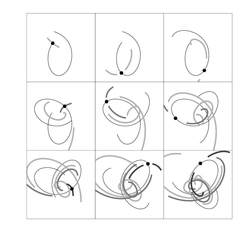
Figure 3: Evolution of debris lost from a satellite over three pericentric passages projected onto the plane perpendicular to the Galactic disk and containing the Sun. In each panel the solid line shows the past and future path of the satellite, and the hexagon shows its position. The panels are equally spaced by 0.22 Gyrs in time, centered on the Galaxy and 100kpc on a side. The grey lines show the positions of the streamers. The bottom left hand panel corresponds to the position and velocity of Sgr today.

In Figure 3 we illustrate the general characteristics of debris dispersal by following a semi-analytic model for the evolution of a satellite with parameters $(f,m_{\rm Sgr},v_{\rm t},v_{\rm circ})=(0.3,10^{9}M_{\odot},242{\rm km/s},174{\rm km/s})$ over three pericentric passages. Each panel is centered on the Galaxy and 100 kpc on a side. The solid line shows the past and future path of the satellite, and the hexagon shows its position. The left hand panels correspond to instants shortly after each pericentric passage (with the bottom left hand panel corresponding to Sgr’s current position and velocity) and the panels in each row are equally spaced between these points in time. The grey ribbons show the location of the debris lost on each pericentric passage. The darkest and shortest pair of ribbons in the final panel correspond to the leading and trailing streamers from the most recent passage (hereafter referred to as passage 0 or by $n_{\rm pass}=0$) and the paired streamers from the preceding passages ( hereafter referred to by $n_{\rm pass}=-1,-2...$) are progressively lighter and longer. Note that the large $m_{\rm Sgr}$ means that the tidal scale $(m_{\rm Sgr}/M_{\rm Gal})^{1/3}\sim 1/10$ is large and so the leading (trailing) streamers are on orbits that come (go) considerably closer to (further from) the Galactic center than the satellite itself. Each of these streamers will have a width less than, but comparable to the amount by which it is offset from the orbit so there will considerable overlap between the populations whose average positions are indicated by the grey lines.

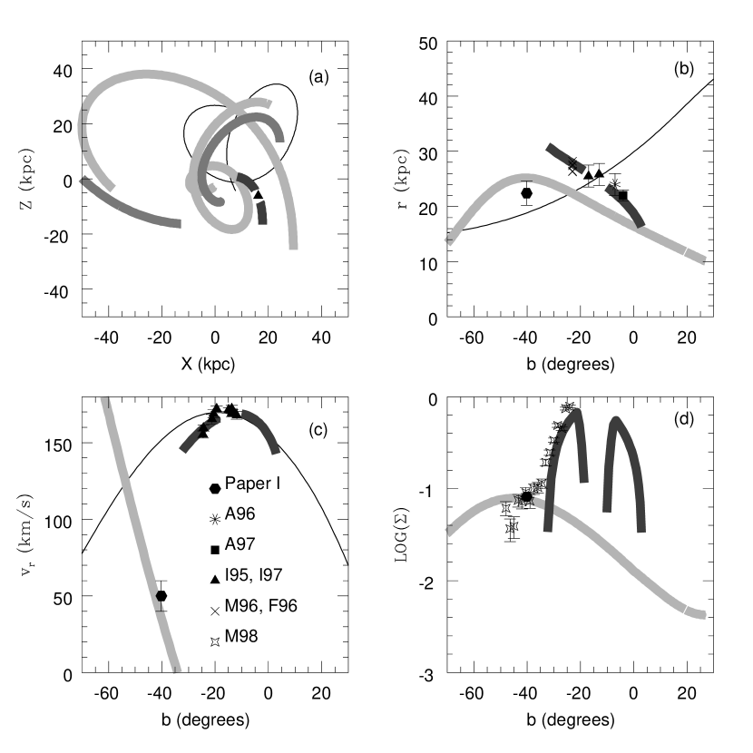
Figure 4: As Figure 1, but with the semi-analytic model also overlaid. Each pair of grey lines represent the locus of a pair of tidal streamers, with the darkest pair being torn from the satellite on the most recent pericentric passage, 50 Myrs ago.

In Figure 4 we repeat Figure 1, but with the predictions of the semi-analytic model shown in Figure 3 overlaid. In the following subsections we use this to illustrate the general successes of using the dynamics of tidal debris to explain the data sets (§3.2). We then go on to discuss whether the current observations can place any stringent limits on the varied parameters (§3.3), and outline the implications for Sgr’s mass loss history (§3.4). Finally, we examine to what extent our discussion will remain valid for non-polar orbits in flattened halo potentials (§3.5).

3.2 Successes of the Models

The location of the streamers (grey ribbons) and the orbit (solid line) projected onto the plane containing the Sun and perpendicular to the Galactic disk are shown in panel (a) of Figure 4. Note that the streamers from the most recent pericentric passage ($n_{\rm pass}=0$) are nearly perpendicular to the orbital path, and that those from the preceding passages ($n_{\rm pass}=-1,-2...$) are clearly separated by a noticeable gap ahead and behind the satellite along its path. This general configuration is apparent in all models, and results from Sgr being only slightly past pericenter in orbital phase — once it reaches apocenter the streamer from passage 0 will spread far enough to overlap in phase with the older ones and the debris will be continuous (see Figure 3). However, currently this means that as we trace the debris back along the orbit of Sgr beyond the extent of material unbound during passage 0 we will not immediately detect material from passage $-1$, but rather debris that has wrapped entirely around the Galaxy and hence must have been torn from Sgr on passages with $n_{\rm pass}\leq-2$, as illustrated by the position of the lightest leading streamer in the Figure.

In panel (b) of Figure 4 we plot the distances to the streamers as seen from the Sun in the direction of the center of the Galaxy as a function of Galactic latitude. Note that the streamers from passage 0 agree very well with the peculiar orientation of material reported in A (96); M (96); F (96) and A (97). The distance estimate we found for our field further down the streamer in Paper I agrees with the prediction for material in the leading streamer from passage $-2$ that has wrapped entirely around the Galaxy to intersect our line of sight. This point serves as a discriminant between the streamers: trailing streamers are offset from the satellite’s path to greater distances and should not be observed so close to the Galactic center; and material in leading streamers from passages with $n_{\rm pass}\leq-3$ will lie progressively closer to the satellite’s orbit (and further from us along the line of sight close to Sgr) at a given orbital phase. These arguments apply to all models.

In panel (c) of Figure 4 we plot the line-of-sight velocity as seen from the Sun in the Galactic rest-frame. The model agrees with the kink in the velocity gradient for the points close to the center of Sgr that was commented on by I (97). The velocity reported at $b=-40^{o}$ in Paper I is too low to agree with a direct extrapolation of the orbit of Sgr over 20^o within the stated error-bars of the proper motion in any of our Galactic models. However, it can be explained consistently within the model where this material is part of a leading streamer from passage $-2$. For a given Galactic model, the distance and velocity of this point, provides the strongest constraint on the orbit of Sgr.

In panel (d) of Figure 4 we show the surface density of each streamer, normalized so that the streamer from passage 0 has the same amplitude as the data in the region reported in M98. In all models, there is a gap of $10^{o}-15^{o}$ between the leading and trailing streamers from passage 0 corresponding to the location of mass still bound to Sgr. The models suggest that the break in slope of the surface density at $b\approx-35^{o}$ corresponds to the end of the streamer from passage 0. The location of this break is dependent on $m_{\rm Sgr}$ and the density of debris beyond this point is sensitive to $f$.

3.3 Limits on Parameters

In order to investigate to what extent the data could limit the parameters we looked at a set of potentials with halo components having $140{\rm km/s}\leq v_{\rm circ}\leq 200$ km/s. In each potential we found the value of $v_{\rm t}$ that allowed the closest fit (by visual inspection) to all the distance and velocity data, except for the tentative velocity measurement at $b=-40^{o}$ (see Paper I for discussion of this point). We considered debris from the last 3 passages alone and did not look at debris from earlier passages because (as noted in the previous section) these streamers would be too distant to fit the point measured at $b=-40^{o}$ in Paper I . In all potentials we could find a value of $v_{\rm t}$ that provided a reasonable fit to these data within the error bars of the proper motion measurement reported in I97. As $v_{\rm circ}$ was increased from 140 km/s to 200 km/s, the necessary $v_{\rm t}$ increased from 205-275 km/s (with a range of about $\pm 10$ km/s about each value) and the time periods and time interval since the most recent pericentric passage decreased from 0.75-0.55 Gyrs and 60-40 Myrs respectively. However, the pericenters and apocenters of the orbits orbits lay in narrow ranges (12-14 kpc and 40-43 kpc). We conclude that although the current observations do not significantly refine our model of the Galactic potential, the proper motion measurement of Sgr, nor the prediction for the time period of its orbit, they do constrain the orbital shape. If we knew the proper motion of Sgr with greater precision we could use the properties of the debris to constrain the Galactic potential more tightly.

Note that the model that fits all the distance and I (97)’s velocity measurements also provides a good match to the uncertain velocity measurement reported in Paper I , even though it was not considered as a constraint. This success supports the tentative identification in Paper I of a group of stars moving at this velocity as indeed being associated with Sgr.

Once we determine a value of $v_{\rm t}$ in each potential we can use the surface density measured in M98 to constrain $m_{\rm Sgr}$. Increasing $m_{\rm Sgr}$ causes the length of each streamer to increase (approximately $\propto m_{\rm Sgr}^{1/3}$). In all potentials considered we found that $m_{\rm Sgr}\sim 10^{9}M_{\odot}$ in order for the streamer from passage 0 to extend to the point where the slope in the surface density profile in M98 changed. M98 estimate a total luminosity associated with Sgr of $\leq 8\times 10^{7}L_{\odot}$ (i.e. including their detections) so this suggests an overall mass-to-light ratio of $\geq 10$, which is consistent with observations of other dwarf spheroidal satellites in orbit around the Milky Way, and with the independent estimates for its mass by I97. However, this large mass is somewhat inconsistent with the measured velocity dispersion of $\sim 10$ km/s along the entire length of Sgr (I (97)). This inconsistency could arise because the finite size of the satellite is ignored in the semi-analytic models, where the debris is effectively being released from the satellite’s center. This simplification would affect the predictions for the length of the tidal streamers from the most recent pericentric passage (passage 0) whose size is comparable to that of the satellite itself, but should be unimportant for the much longer streamers from earlier passages.

Finally, we found that $f$ was required to be in the range $0.2\leq f\leq 0.3$ in order for the relative amplitude of debris at either side of the break in the slope of the surface density profile approximately to be fit by material in the streamers from passages 0 and $-2$.

3.4 Mass Loss History and Future Survival

One question that has been addressed repeatedly since Sgr’s discovery is whether we are witnessing its death throes or will Sgr survive another passage. The models that best fit the data described in the previous section had $0.2\leq f\leq 0.3$, which means that Sgr has lost between half and two-thirds of its mass over the last three pericentric passages (or 1.1-1.5 Gyrs depending on the Galactic potential). We can crudely check this picture by assuming that our success in modeling the distance and velocity features means that Sgr is dominated by unbound material beyond at least $10^{o}$ from its center. M98 report that the surface brightness (in mag/arcsec^-2) of their points between $10^{o}$ and $20^{o}$ from Sgr can be fitted by a function $\Sigma_{v}\propto 0.23\theta$ (where $\theta$ is the separation from the center of Sgr in degrees) which agrees with the central surface brightness of Sgr when extrapolated inwards. If mass follows light, this suggests that the mass surface density will fall as $\Sigma\propto\exp(-\theta/10)$. Hence, if Sgr and its debris have roughly constant width along its orbit the ratio of the mass between $10^{o}\leq\theta\leq 20^{o}$ (i.e. in the streamers from passage 0) to that within $\theta=10^{o}$ will be $\sim exp(-1)=0.37$, in rough agreement with our assumed fractional mass loss rates. Such a large mass loss rate rules out the picture where Sgr is merely distorted by the Milky Way’s tidal field with very little evolution and suggests that Sgr is unlikely to survive many more pericentric passages. This mass loss rate corresponds to a decrease in Sgr’s luminosity in the last 1.1-1.5 Gyrs alone that is of order 10% of the total luminosity of the stellar halo ($\sim 10^{9}L_{\odot}$, see Freeman (1996)).

3.5 Halo Flattening and Non-Polar Orbits

We have so far limited our discussion to polar orbits in potentials with exactly spherical halos. Non-polar orbits in a flattened halo potential (i.e. setting $q<1$ in equation [3]) will precess and disturb the alignment of the leading and trailing streamers. In principle, we could use the apparent precession of the debris at different points along the streamers to place limits on both the direction of the proper motion and the degree of flattening of the Galaxy’s potential. However, the strongest constraints on these quantities would come from detections (or lack of detections) farthest from the center of Sgr (e.g. M (98); Paper I ) which are currently the most uncertain. Hence, we do not try to place limits on these dimensions of parameter-space, and instead simply examine to what extent our discussion of debris evolution in a spherical halo will remain valid in the non-spherical case.

Figure 5 contours the projected angular difference between Sgr and a point $2\pi$ ahead along it’s orbit. The orbits were run in halo potentials with different $q$ and with initial radial velocity and motion perpendicular to the Galactic disk set by I (97)’s observations, but with motions perpendicular to the line of sight and parallel to the Galactic disk $v_{\phi}$ allowed to vary. The positive (solid) and negative (dotted) contours are spaced by 5 degrees. This plot provides upper limits to the apparent orbital precession of material in the leading streamer since debris on orbits more tightly bound to the Galaxy than Sgr would lie closer to the Galactic center than it’s orbit and hence have smaller angular separations from Sgr when seen from the Sun in projection. Figure 5 clearly cautions that our identification of M (98)’s and Paper I ’s detections as material in the leading streamer could be wrong if $q<0.9$ and $|v_{\phi}|>20$ km/s. Although this condition appears to be rather restrictive, note that this modest potential flattening translates to an axis ratio $\sim 0.7$ in the corresponding density distribution (see Binney & Tremaine 1987, equation 2-55b). In comparison, a recent study combining limits from stellar-kinematics and from the flaring of gas out of the Galactic plane constrains the dark matter halo to have an axis ratio in density of $0.75\pm 0.25$ (Olling & Merrifield (1998)).

4 Summary and Conclusions

In this paper, we have combined all observations of Sgr that have been reported in the literature since 1994 and directly compared them to semi-analytic models of the dispersal of material once it becomes unbound from a satellite. By varying the circular velocity of the halo component of our Milky Way potential along with Sgr’s transverse velocity, current mass and mass loss rate, we have found that:

1. The current data cannot constrain the Milky Way potential and Sgr’s transverse velocity independently, but do favor specific orbital characteristics: the orbits of the best fit models all had pericenters $\sim 13$kpc, apocenters $\sim 41$kpc, radial time periods $\sim 0.55-0.75$Gyrs and time since the most recent pericenter $\sim 40-60$ Myrs. If the proper motion of Sgr were known with greater precision, the data could be used to constrain the Galactic potential more tightly. Note that Murali & Dubinski (1999) also found that poor knowledge of proper motion was the limiting factor to using globular cluster tidal tails to measure the Galactic potential.

2. All the peculiar features in the data could be explained with the dynamics of unbound material:

   • The orientation of material perpendicular to Sgr’s orbit close to its center reported in A (96, 97) and Paper I , and the kink in the radial velocities reported in I (97) are consistent with the predicted locus of debris from the most recent pericentric passage.

   • The radial velocity and distance measurements of material at $b=-40^{o}$ reported in Paper I correspond to those expected for material in a leading streamer that has wrapped entirely around the Galaxy to intercept our line of sight. The density of this material in this region dominates over trailing material because there is a clear gap between material stripped from the most recent and immediately preceding pericentric passages.

   • The break in the slope of the surface density profile reported in M (98) naturally occurs in our model at the transition between material in the trailing streamer from the most recent passage and the leading streamer that has wrapped around the Galaxy.

3. Models that are consistent with the data have current masses of Sgr of $\sim 10^{9}M_{\odot}$, and mass loss rates such that Sgr was 2-3 times larger $\leq 1.5$Gyrs ago. This mass loss rate corresponds to a decrease in Sgr’s luminosity that is of order 10% of the total luminosity of the stellar halo and suggests Sgr is unlikely to survive many more pericentric passages.

We consider the general scenario outlined in our first two points to be fairly robust, provided the halo potential is not highly flattened (see §3.5). The specific model for the mass and mass loss rate in the third point is more tentative. Future observations should reveal the history of Sgr in greater detail. Velocity measurements along the entire length of M (98)’s data set would clearly confirm or rule out our identification of this material as part of the leading streamer and distance estimates would indicate whether we are indeed seeing only material wrapped around the Galaxy from the pericentric passage $\sim 1.1-1.5$ Gyrs ago (i.e. $n_{\rm pass}=-2$), or if we might also be seeing material (a few kpc more distant) from earlier passages. The absence of debris from these earlier passages in M98’s data set could provide support for Zhao’s (1998) model of Sgr’s history, which requires Sgr to be on a much less tightly bound orbit before suffering a collision with the LMC 2 Gyrs ago. This scenario limits the number of close encounters with the Milky Way that Sgr has undergone, and hence the number of streamers from different passages associated with it. On the other hand, if Zhao’s model can clearly be ruled out, we instead face the task of building a consistent picture in which Sgr has orbited the Galaxy many times and is only now being completely destroyed.

Additional detections (ideally with distance, velocity and surface density estimates) or lack of detections of stars associated with Sgr in fields in the Northern Galactic hemisphere (e.g. Paper I ) or radial velocity measurements along M (98)’s data set would allow us to pin down Sgr’s path, which in turn would more precisely constrain both the shape and depth of the Galactic potential and Sgr’s proper motion. Unfortunately, the converse of this statement is that our poor knowledge of Sgr’s motion parallel to the Galactic disk and our uncertainty about the degree to which the Galaxy’s potential is flattened mean that any predictions of where to find such streamers are very imprecise. However, the recently discovered carbon star stream (Irwin & Totten 1999) could provide a starting point for such studies — a preliminary analysis of the carbon star data set alone suggests that the halo potential is near spherical (private communication from Rodrigo Ibata). Further into the future the GAIA satellite (Global Astrometric Imager for Astrophysics — to be launched in 2009) will provide proper motions of all stars brighter than 20th magnitude with $\sim 5-200\mu as/$yr accuracy and allow us easily to distinguish Sgr’s debris across the sky from foreground contaminants.

Finally, we caution that the results reported here are only intended as a guide to the probable history of Sgr and that more detailed velocity and distance information along its streamers is needed to come to firmer conclusions. The semi-analytic models are not exact, and, with more data to use as constraints, any results should ideally be confirmed using N-body simulations that also take into account the effect of dynamical friction. Nevertheless, this study illustrates the tremendous power of using debris, rather than the properties of bound material, to understand the history of satellite galaxies.

Figure 1: Summary of data used in this investigation. Panel (a) shows the current position (triangle) and a possible orbit (solid line) of Sgr projected onto the plane perpendicular to the Galactic disk and containing the Sun at $(X,Z)=(-8,0)$kpc. The arrow indicates its direction of motion. Panels (b), (c) and (d) show the distance from the Sun, line-of-sight velocity in a Galactic rest frame and surface density of the data points plotted against their Galactic latitude. The orbit is again overlaid in Panels (b) and (c). The sources of the data points are coded with the same symbols in each panel, as labeled in Panel (c).

Figure 2: Top panel — the velocity of a circular orbit in the disk plane at distance $R$ from the Galactic center for the Galactic model given in equation (1) with $v_{\rm circ}=140,174,200$ km/s. Bottom panel — the mass enclosed within distance $R$ for the same models.

Figure 5: Positive (solid) and negative (dotted) contours of angular precession of orbit, as a function of the flattening $q$ of the halo potential and the velocity of Sgr perpendicular to the line of sight and parallel to the plane of the Galactic disk $v_{\phi}$. The levels are spaced by 5 degrees.

References

- A (96) Alard, C. 1996, ApJ, 458, L17 (A96)
- A (97) Alcock, C., Allsman, R., Alves, D. Axelrod, T., Becker, A., Bennett, D., Cook, K., Guern, J., et al. 1997, ApJ, 474, 217 (A97)
- Binney & Tremaine (1987) Binney, J. & Tremaine, S. 1987, Galactic Dynamics (Princeton University Press, Princeton)
- F (96) Fahlman, G., Mandushev, G., Richer, H., Thompson, I. & Sivaramakrishnan, A. 1996, ApJ, 459, L65 (F96)
- Freeman (1996) Freeman, K. C. 1996, in The Formation of the Galactic Halo: Inside and Out, ASP Conf. Ser. Vol 92, eds. H. Morrison & A. Sarajedini, (ASP, San Francisco), p. 3
- Ibata & Lewis (1998) Ibata, R. A. & Lewis, G. F. 1998 ApJ, 500, 575
- I (94) Ibata, R., Gilmore, G. & Irwin, M. 1994, Nature, 370, 194 (I94)
- I (95) Ibata, R. A., Gilmore, G. & Irwin, M. J. 1995, MNRAS, 277, 781 (I95)
- I (97) Ibata, R., Wyse, R., Gilmore, G., Irwin, M. & Suntzeff, N. 1997, AJ, 113, 634 (I97)
- Irwin & Totten (1999) Irwin, M.J. & Totten, E. 1999, in preparation
- Johnston (1998a, 1998b) Johnston, K. V. 1998a, ApJ, 495, 297
- (12) Johnston, K. V. 1998b, to appear in ASP Conference Ser, “The Galactic Halo”, eds. Putman and Gibson