The Initial Mass Function of the Galactic Bulge
Down to $\sim 0.15\,\hbox{$M_{\odot}$}$

Abstract

We present a luminosity function (LF) for lower main sequence stars in the Galactic bulge near $(l,b)=(0^{\circ},-6^{\circ})$ to $J=24$, corresponding to $M_{J}\sim 9.3$. This LF is derived from Hubble Space Telescope (HST) + Near Infrared Camera and Multi Object Spectrometer (NICMOS) observations of a region of $22\hbox{\hbox to0.0pt{\hbox{.}\hss}\hbox{${}^{\prime\prime}$}}5\times 22\hbox{\hbox to0.0pt{\hbox{.}\hss}\hbox{${}^{\prime\prime}$}}5$, with the F110W and F160W filters. The main sequence locus in the infrared shows a strong change in slope at $J\sim 20.5$ ($M_{\rm J}\sim 5.75)$ which is well fit by new low mass models that include water and molecular hydrogen opacity. Our derived mass function (which is not corrected for binary companions) is the deepest measured to date in the bulge, and extends to 0.15 $M_{\odot}$ with a power law slope of $\alpha=-1.33\pm 0.07$; a Salpeter mass function would have $\alpha=-2.35$. We also combine our $J$ band LF with previously published data for the evolved stars to produce a bulge LF spanning $\sim$ 15 magnitudes. We show that this mass function has negligible dependence on the adopted bulge metallicity and distance modulus. Although shallower than the Salpeter slope, the slope of the bulge IMF is steeper than that recently found for the Galactic disk ($\alpha=-0.8$ and $\alpha=-0.54$ from the data of Reid & Gizis, 1997, and Gould et al. 1997, respectively, in the same mass interval), but is virtually identical to the disk IMF derived by Kroupa et al. (1993). The bulge IMF is also quite similar to the mass functions derived for those globular clusters which are believed to have experienced little or no dynamical evolution. Finally, we derive the $M/L_{J}$ ratio of the bulge to be $\sim 0.9\pm 0.1$ $M_{\odot}/L_{\odot}$, and briefly discuss the implications of this bulge IMF for the interpretation of the microlensing events observed in the direction of the Galactic bulge.

1 Introduction

The initial mass function (IMF) is a fundamental property of stellar populations, hence one of the most crucial ingredients in models of galaxy formation and evolution. It determines several key properties of stellar populations and galaxies, such as the yield of heavy element production, the luminosity evolution over time, the mass-to-light ratio, the total star formation rate at low and high redshifts as inferred from empirical estimators, and the energetic feedback into the interstellar medium. Yet, the IMF is usually taken as a free parameter, particularly at the low-mass end (for recent reviews on the IMF see Larson 1998; Scalo 1998, 1999). Observational constraints on the IMF are therefore of the greatest astrophysical importance.

Knowing the IMF at $M{\mathrel{\mathchoice{\lower 2.9pt\vbox{\halign{$\m@th\displaystyle\hfil#\hfil$\cr<\crcr\sim\crcr}}}{\lower 2.9pt\vbox{\halign{$\m@th\textstyle\hfil#\hfil$\cr<\crcr\sim\crcr}}}{\lower 2.9pt\vbox{\halign{$\m@th\scriptstyle\hfil#\hfil$\cr<\crcr\sim\crcr}}}{\lower 2.9pt\vbox{\halign{$\m@th\scriptscriptstyle\hfil#\hfil$\cr<\crcr\sim\crcr}}}}}1M_{\odot}$ in spiral bulges and elliptical galaxies is of special interest because these spheroids contain a large fraction, perhaps a majority, of all the stellar mass of the universe (e.g., Fugugita, Hogan & Peebles, 1998). However, there is presently no way to directly determine the IMF of spheroids except by measuring the luminosity function (LF) of our own bulge as the only surrogate for the unresolvable population in other galaxies. Although the low mass end of the stellar IMF has been determined for the solar neighborhood (Kroupa, Tout & Gilmore 1993; Gould, Bahcall & Flynn 1997; Reid & Gizis 1997) and in young open clusters (Hillenbrand 1997; Bouvier et al. 1998; Luhman et al. 1998) it is only in the Galactic bulge that one can be confident that the stellar population is old, largely coeval, and metal rich (Whitford 1978; Ortolani et al. 1995; Mc William & Rich 1994), i.e., the closest we can come in a nearby, resolved stellar population to what prevails in other spiral bulges and elliptical galaxies (Renzini 1999).

The recent discovery of a high rate of microlensing events towards the bulge (Udalski et al. 1994; Alcock et al. 1997) has made the determination of the faint end of the IMF a yet more urgent problem. In brief, if the bulge IMF is close to that of the solar-neighborhood (Gould et al. 1997) then the bulk of the short ($\sim 10$ day) microlensing events would remain unexplained, perhaps requiring a large population of brown dwarfs (Han 1997). However, an IMF extending to the H-burning limit with a Salpeter law can account for both the total mass of the bulge and the frequency of microlensing events (Zhao, Spergel, & Rich 1995). It is therefore tempting to suspect that the bulge and solar-neighborhood IMFs are different. However, the interpretation of the microlensing events relies on assumptions about the phase-space distribution of both the lenses and sources, and some events may be caused by collapsed stars, brown dwarfs or even non-stellar objects. Therefore, the most reliable way to resolve these ambiguities (and thus maximize the information from microlensing itself) is to obtain a representative stellar inventory of the bulge from star counts, and to incorporate this into the microlensing analysis.

A recent determination of the bulge IMF down to $M\sim 0.35M_{\odot}$ has been provided by Holtzman et al. (1998), based on Hubble Space Telescope (HST) + Wide Field and Planetary Camera (WFPC2) observations of Baade’s Window. Globular clusters offer another approach towards determining the IMF for $M{\mathrel{\mathchoice{\lower 2.9pt\vbox{\halign{$\m@th\displaystyle\hfil#\hfil$\cr<\crcr\sim\crcr}}}{\lower 2.9pt\vbox{\halign{$\m@th\textstyle\hfil#\hfil$\cr<\crcr\sim\crcr}}}{\lower 2.9pt\vbox{\halign{$\m@th\scriptstyle\hfil#\hfil$\cr<\crcr\sim\crcr}}}{\lower 2.9pt\vbox{\halign{$\m@th\scriptscriptstyle\hfil#\hfil$\cr<\crcr\sim\crcr}}}}}1M_{\odot}$, and deep HST observations are indeed providing important information on their present-day mass functions (De Marchi et al. 1999; Piotto & Zoccali 1999, and references therein). However, clusters suffer from dynamical evolution and evaporation of low-mass stars, and therefore there is no model-independent way to infer their IMFs from their observed present day mass function (MF).

Because faint, low-mass stars have such low temperatures, infrared observations give a crucial advantage over optical data. Moreover, in the near-IR the effects of extinction and differential reddening are considerably reduced, and the bolometric luminosities of M dwarfs (the vast majority of the sampled stars) are best determined in the near-IR both because of their cool temperatures and severe molecular blanketing in the optical. Finally, the relatively low IR background of HST, combined with diffraction limited resolution, gives a fundamental advantage when dealing with very faint sources in a crowded field. Therefore, the NICMOS near-IR cameras offer a unique opportunity to reach the faintest stars possible in the Galactic bulge, thus extending to lower masses the range over which the IMF is observationally constrained.

In order to ensure the success of the project we paid special attention to the selection of the bulge field to be observed. The most widely studied field in the Galactic bulge is the $b=-4^{\circ}$ field known as Baade’s Window. However, for the NICMOS observations we did not choose to point HST at this field. A priori, in Baade’s Window, crowding might have been too severe to confidently undertake this experiment that aims at counting the faintest bulge stars in the frame. At $b=-4^{\circ}$ the average surface brightness (corrected for $A_{\rm V}\simeq 1.2$ mag extinction) is 18.7 $V$ mag arcsec^-2 (Terndrup 1988), and with a true modulus of 14.5 mag one samples $M_{\rm V}=4.2$ mag arcsec^-2, corresponding to a bolometric luminosity of $\sim 2.8L_{\odot}\,$arcsec^-2 (using population synthesis models, e.g., by Maraston 1998). Hence, the NIC2 camera samples a total bolometric luminosity $L_{\rm T}\simeq 10^{3}L_{\odot}$. This allows one to estimate the number of main sequence stars in a HST NIC2 frame, knowing that for a $\sim 15$ Gyr old population the scale factor in the IMF – $\psi(M)=AM^{\alpha}$ – is given by $A\simeq 1.2L_{\rm T}$ (Renzini 1998). Integrating the IMF from 0.1 to 0.9 $M_{\odot}$, with $\alpha=-2.35$ (the Salpeter IMF slope), and $A=1.2\times 10^{3}$, we get that a NIC2 frame will contain $\sim 2.3\times 10^{4}$ stars. Since the NIC2 camera has $6.55\times 10^{4}$ pixels, while selecting the target field we therefore concluded that accurate photometry would have been difficult towards the faint end of the LF, if the IMF were to follow the Salpeter’s slope all the way to the hydrogen burning limit.

For our observations we selected instead the field at $b=-6^{\circ}$, where the surface brightness is $\sim 1$ mag lower, and then we expect $\sim 2.5$ times fewer stars in a NIC2 frame compared to Baade’s Window, significantly improving the stars/pixel number ratio. Although more distant from the nucleus than Baade’s Window, the field population is still dominated by the metal rich stars characteristic of the bulge, as shown by the strongly descending red giant branch in the $(V,V-I)$ diagram (Rich et al. 1998), which makes sure that we are properly studying the metal rich bulge in this location. Moreover, photometry down to the hydrogen burning limit should not be compromised by crowding, especially if the IMF were to flatten out below the Salpeter’s slope as in the solar neighborhood (Gould et al. 1997), implying a smaller number of low-mass stars.

2 Observations and Data Analysis

The selected field (RA=18:11:05, DEC=$-$31:45:49 (J2000); $l$=0.277, $b$=$-$6.167) was observed with the NIC2 camera of NICMOS, on board HST, through the filters F110W and F160W. Parallel observations with NIC1 were collected through the F110W filter. Fourteen orbits were allocated, for total NIC2 integration times of 10240 s and 25600 s in F110W and F160W, respectively. Only the F110W filter was used for the NIC1 parallel observations, for a total integration time of 35850 s. All exposures were obtained using the MULTIACCUM readout mode and the STEP64 time sequence through an eight-position spiral dithering with size of $0\hbox{\hbox to0.0pt{\hbox{.}\hss}\hbox{${}^{\prime\prime}$}}4$. The pixel size of the NIC2 detector is $0\hbox{\hbox to0.0pt{\hbox{.}\hss}\hbox{${}^{\prime\prime}$}}075$, giving a field of view of $19\hbox{\hbox to0.0pt{\hbox{.}\hss}\hbox{${}^{\prime\prime}$}}2\times 19\hbox{\hbox to0.0pt{\hbox{.}\hss}\hbox{${}^{\prime\prime}$}}2$ for each frame. Small offsets and rotations among the frames gave us a slightly larger total field ($22\hbox{\hbox to0.0pt{\hbox{.}\hss}\hbox{${}^{\prime\prime}$}}5\times 22\hbox{\hbox to0.0pt{\hbox{.}\hss}\hbox{${}^{\prime\prime}$}}5$). Figure 1 shows the observed bulge region as it appears in a combination of all the frames.

The images were bias subtracted, dark corrected and flat-fielded by the standard NICMOS pipeline CALNICA. This routine also combines the multiple readouts of the MULTIACCUM mode, giving an output image which is expressed in counts per second per pixel. We therefore multiplied each of these images by its total exposure time, so that the photometry software would measure the correct signal-to-noise ratio (S/N).

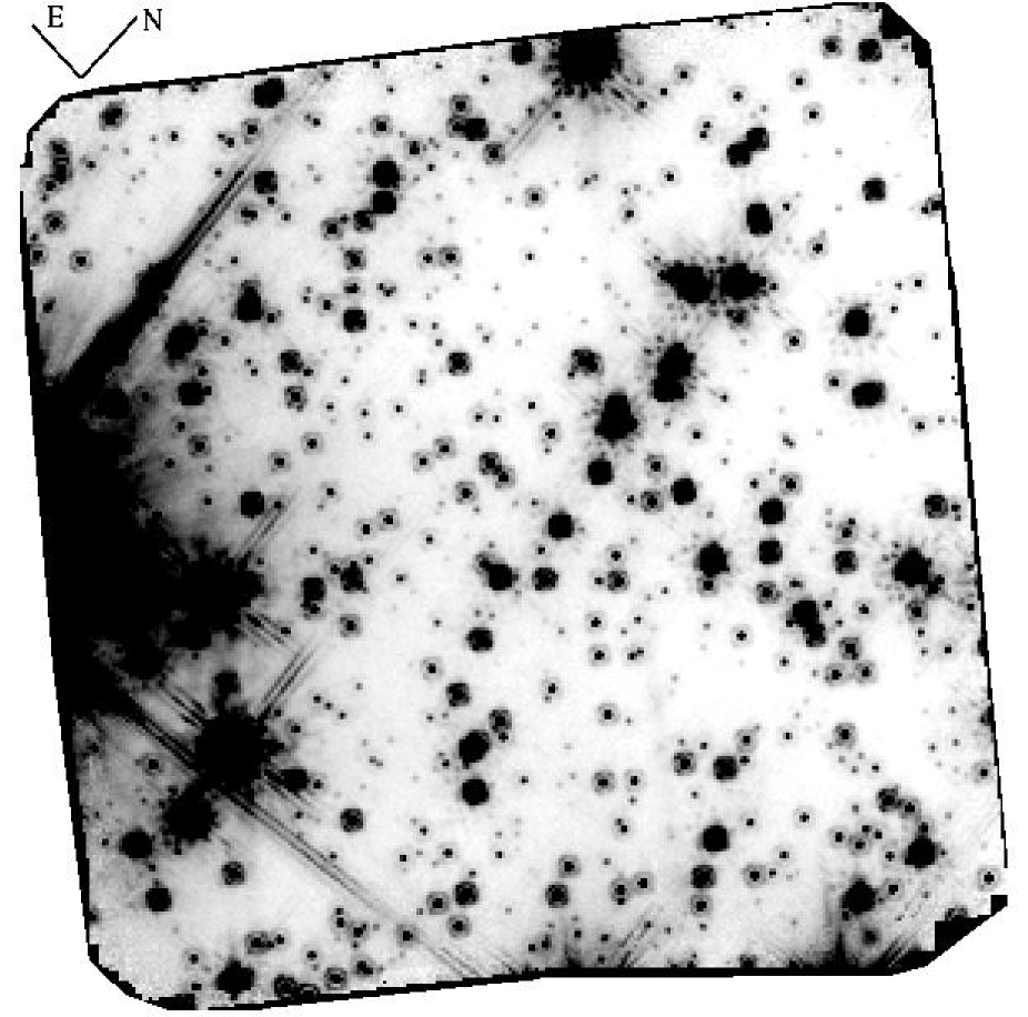
Figure 1: Negative image of the region of the bulge window at $-6^{\circ}$ observed with the NIC2 camera of NICMOS on board HST . This image is obtained from the combination of all the F110W and F160W frames. The total field of view is about $22\hbox{\hbox to0.0pt{\hbox{.}\hss}\hbox{${}^{\prime\prime}$}}5\times 22\hbox{\hbox to0.0pt{\hbox{.}\hss}\hbox{${}^{\prime\prime}$}}5$.

The data quality file corresponding to each image was used to mask out the saturated and bad pixels by setting them to a very high value, that was discarded in the photometry. Following the NIC2 manual, the read-out noise of each frame was assumed to be 32 electrons, corresponding to 6.1 ADU, with a conversion factor of 5.4 $e^{-}/$ADU. The mean sky level of each 640 s exposure was $\sim 50$ and $\sim 40$ ADU in F110W and F160W respectively. That is, the noise is dominated by read noise rather than the sky.

Preliminary star finding and aperture photometry was carried out on each frame using the DAOPHOTII photometry package (Stetson 1987). We then used all the stars identified in each frame to obtain the coordinate transformations among all the frames. These transformations were used to register the frames and obtain a median image. The latter, having the highest S/N, was used to create the most complete star list, by means of two complete runs of DAOPHOTII and ALLSTAR. The final star list, together with the coordinate transformations, was finally used as input for ALLFRAME (Stetson 1994), for the simultaneous reduction of all the frames. Particular attention was devoted to modeling the NIC2 point spread function (PSF) in the two filters. This was performed using specific software (MULTIPSF), provided by P.B. Stetson, that allows measurement of a unique PSF from the brightest and most isolated stars in a set of different frames. Assuming that the PSF profile does not change from frame to frame, we were able to measure the same $\sim 30$ stars in all the frames of each filter. The spatial dithering allowed us to measure the selected stars in different locations on the chip, centered in different positions inside a pixel, so the final PSF was of considerably better quality than the one we could obtain for each frame taken individually. The stellar full width at half maximum is $\sim 1.5$ pixels while the adopted model PSF was defined up to a 14 pixels radius.

Aperture corrections were empirically determined on the most isolated stars, and applied to the ALLFRAME measures in order to obtain the stellar magnitudes in a $0\hbox{\hbox to0.0pt{\hbox{.}\hss}\hbox{${}^{\prime\prime}$}}5$ aperture. The magnitudes were then converted to count rates, and multiplied by 1.15 to correct to an infinite aperture. The inverse sensitivity, given as the keyword PHOTFLAM in the header of the images, together with the zero points PHOTZPT given in Table 2 of Stephens et al. (1999), were used to convert the count rates into HST $m_{110}$ and $m_{160}$ magnitudes. The latter were then transformed in the CIT/CTIO system according to the calibration equations determined by Stephens et al. (1999) from the comparison between NICMOS and ground-based observations of the same 14 bright stars. As discussed by Stephens et al. (1999), this calibration is consistent (over the common color range) with the one described in the NICMOS calibration documentation.

A second, independent reduction of the data was carried out with the same software (DAOPHOTII/ALLSTAR) but with somewhat different procedures. Nearly identical results were obtained as in the first reduction. In this reduction we performed simple star finding and PSF fitting on each individual frame but without using the median image, or ALLFRAME. The resulting photometry is somewhat shallower but it provides a useful consistency check both in terms of magnitudes and numbers of identified stars, in the common magnitude range. Figure 2 shows the comparison between the (calibrated) output photometry of the two procedures. The two bottom panels show that, for the stars identified in both cases (i.e., except for the fainter ones, identified only by ALLFRAME) the measured magnitudes are in very good agreement, with a very small offset $\Delta J=0.01$, due to some systematic error in one (or both) of the aperture corrections. The $H$ magnitudes of the brightest stars ($H<17.6$) also differ by $\Delta H\sim 0.05$. The top panel shows the two LFs (before completeness correction) which are almost identical down to $J=23$, where the ALLFRAME reductions go significantly deeper.

Figure 2: Comparison between the results of ALLFRAME, as described in § 2 (index ALLF) and the results of the standard DAOPHOTII/ALLSTAR procedure (index ALLS).

3 The Color–Magnitude Diagram

The observed color–magnitude diagram (CMD) for the 780 stars measured in our $22\hbox{\hbox to0.0pt{\hbox{.}\hss}\hbox{${}^{\prime\prime}$}}5\times 22\hbox{\hbox to0.0pt{\hbox{.}\hss}\hbox{${}^{\prime\prime}$}}5$ field is shown in Figure 3. Only the stars identified in at least 5 independent frames per filter are plotted. A further selection on the magnitude error and on the sharp parameter was imposed to discard spurious detections due to noise and intersecting diffraction spikes that may remain around the brightest stars. The bulge main sequence (MS) is well defined from the turnoff ($J\sim 18$) down to magnitude $J\sim 24$ where the sequence starts to broaden and the density of stars falls abruptly. A prominent feature in this CMD is the sharp bend that is clearly visible at $J\approx 20.5$. Fainter than this point, the MS is almost vertical. As predicted by stellar models (Cassisi et al. 1999; Baraffe et al. 1997), this behavior is due to the competition between the tendency towards redder colors due to both the decreasing effective temperature and the increasing molecular absorption at optical wavelengths, and the increasing collision-induced absorption of molecular hydrogen at infrared wavelengths (CIA mechanism, Saumon et al. 1994).

The two brightest stars in the CMD of Figure 3, located in the left side of our field (Fig. 1), were saturated; their magnitudes have been measured independently by extrapolating their PSF profiles into the central region.

Figure 3: The observed color–magnitude diagram of the 780 stars in the NIC2 field. The solid line is the isochrone for a solar metallicity, 10 Gyr old population (Cassisi et al. 1999). The labels on the left indicate the values of absolute distance modulus and reddening taken from the literature (Rich et al. 1998), while the values on the right quote the corresponding quantities in the infrared bands, adopted for this comparison. The shift to redder colors of the isochrone at $J\sim 20.5$ ($M_{\rm J}\sim 5.75$) is caused by the appearance of opacity from water and molecular hydrogen.

Also shown in Figure 3 is the theoretical isochrone by Cassisi et al. (1999). These models have been constructed by adopting the most updated input physics, such as stellar opacities, equation of state, and outer boundary conditions (see Cassisi et al. 1999, for more details). We adopt here the absolute distance modulus and reddening of this region of the Galactic bulge, as measured by Rich et al. (1998): $(m-M)_{0}=14.38$ and $E(B-V)=0.41$. By assuming $R_{V}=3.1$ the extinction is $A_{V}=1.27$, which can be converted to the corresponding $A_{J}$ and $A_{H}$ by means of the relations given by Cardelli et al. (1989): $A_{J}=0.282A_{V}$ and $A_{H}=0.190A_{V}$. The isochrone shown in Figure 3 refers to solar metallicity ([Fe/H]=[$\alpha$/Fe]=0) and an age of 10 Gyrs. The model is a satisfactory match to the general shape of the observed MS, in particular the position of the bend at $J\sim 20.5$ ($M_{\rm J}\sim 5.75$) is well reproduced, even if its strength seems to be a little overestimated. This feature also provides a good check of the zero point of the photometric calibration and the adopted distance and reddening.

The present NICMOS data provide a too sparse sampling of the turnoff area for properly addressing the issue of the age of the bulge stellar populations. This will be attempted in a future paper, combining our NICMOS data with deep WFPC2 observations of the same field, as well as wide field $V$ and $I$ observations taken at the ESO/MPIA 2.2m telescope (Zoccali et al. 1999).

4 The Luminosity Function

In order to obtain the stellar LF of our field, particular attention was devoted to estimating the completeness of our sample. Standard artificial-star tests were carried out on the NIC2 field, in the same way as described in detail by Piotto & Zoccali (1999). We performed ten independent tests, by adding about seventy stars each time, with magnitudes in the range $20<J<25$. Visual inspection of the stars-subtracted image insured that our photometry was complete for brighter magnitudes. The artificial stars were arranged in a spatial grid such that the separation between the centers of each star pair was two PSF radii plus one pixel. This allowed us to add the maximum number of stars, without creating overcrowding. In addition, the position of each star in the grid was randomly located inside one pixel, so as to prevent the centers of all the artificial stars from falling on the same position within a pixel, which would have biased their probability of being detected. The artificial stars were added on each individual $J$ and $H$ image. It should be noticed that the stars must be added in the same position on the sky, therefore their coordinates must be different in different frames, following the frame-to-frame coordinate transformations calculated from the original photometry. A high precision is required in this process, in order to be able to measure the artificial stars with the same photometric accuracy of the original ones. We then ran the same photometry procedure used for the original photometry: star finding was performed on the median of all the star–added images, and then ALLFRAME was used for the simultaneous photometry of all the frames. The same selection criteria used for the original stars were applied to the output list of the artificial star tests.

Figure 4: The LF extracted from the CMD of Fig. 3. The LF before the completeness correction is shown as a dotted histogram. Error bars are the quadratic sum of the Poisson error on the raw star counts and the error in the completeness corrections. The faintest bin was not used in the derivation of the IMF, because of its low completeness.

The completeness correction obtained in this way was applied to the LF obtained from the CMD of Figure 3. This procedure also automatically compensates for the differences of the total integration time across the $22\hbox{\hbox to0.0pt{\hbox{.}\hss}\hbox{${}^{\prime\prime}$}}5\times 22\hbox{\hbox to0.0pt{\hbox{.}\hss}\hbox{${}^{\prime\prime}$}}5$ field. It is worth noting that the scatter in the color of the stars on the right of the main sequence, for $J>21$, is also present in the CMD for the artificial stars, which indicates that the effect is spurious. Visual inspection of these stars on the image revealed that they are all located on the left side of the field, where scattered light from a few very bright objects is also present. Some of them could be residual noise spikes, but some are likely to be real stars whose magnitude has been enhanced due to the proximity of brighter stars. The fact that these objects are present only on the right side of the main sequence indicates that such effect is stronger for the $H$ magnitudes, a likely result of the poorer PSF in the $H$-band. The way in which we applied the completeness correction (i.e. determining the completeness fraction as a function of the recovered magnitude of the artificial stars, instead of the input magnitude) automatically takes into account the effect of the migration of the stars towards brighter magnitudes, therefore we didn’t impose any further selection on the CMD of Figure 3. The resulting $J$-band LF is shown in Figure 4; it is very smooth over the whole range from the bin at $J=18$ (turnoff region) to the faint limit at $J=24$. Also shown as a dotted histogram is the raw LF, without completeness correction. In the determination of the IMF, we did not use the first two bins that, according to our model, correspond to evolved stars, nor the very last bin ($J=24.25$) because its completeness is $\sim 30\%$. The second to last bin, at $J=24$, is complete at $46\%$.

Since the field is located at low Galactic latitude, contamination by disk stars cannot be neglected. We offer an estimate of this contamination using Kent’s (1992) model for the $K$ band luminosity distributions of the disk and bulge. If the LFs of the disk and bulge have the same form as the observed LF in our field, scaled for distance and stellar density, then we find that about 11% of the stars in our field are disk stars, with a modest trend from about 9% at the faint end ($J\sim 24$), to about 14% at the bright end ($J\sim 17$) of the LF in Figure 10. We then adopt an overall reduction of the LF by 11% for $J>17$. We note, however, that this is only a rough estimate of the disk contamination. Available data do not allow a more accurate correction, and further optical and IR data would be required to address this problem more properly. The LF of Figure 4 is listed in Table 1. Column 1 gives the $J$ magnitude, Column 2 and 3 give the raw and completeness corrected counts, respectively, Column 4 is the error, and Column 5 the estimated contribution from disk stars.

Contamination by extragalactic objects is estimated using the NICMOS $H$-band galaxy counts (Yan et al. 1998). This gives less than one galaxy for $J<23$, and between 1.2 and 2.9 galaxies in the last two bins of our LF, corresponding to $J=23.5$ and $J=24$, respectively. We therefore conclude that this source of contamination can be neglected in our analysis.

5 NIC1 data

Figure 5: Comparison between the LF extracted from the NIC2 and NIC1 data. Neither data set is corrected for incompleteness. The two LFs are very similar, down to magnitude $J\approx 23$ where the NIC1 LF falls abruptly due primarily to the by eye selection adopted to eliminate spurious detections.

An additional set of data on a nearby bulge field is provided by our parallel observations with the NIC1 camera through the F110W filter. The field of view of NIC1 is significantly smaller ($11^{{}^{\prime\prime}}\times 11^{{}^{\prime\prime}}$) than that of NIC2, but thanks to its smaller pixel size (0.^′′043), it allows more accurate sampling of the PSF and therefore it yields more accurate photometry for stars with good photon statistics. In our case, due to the rotation of the NIC2 field in different visits, the NIC1 camera actually mapped a larger region ($16^{{}^{\prime\prime}}\times 14^{{}^{\prime\prime}}$). The use of only one filter has the disadvantage that it is not possible to construct a CMD, but allowed a longer exposure time (35850 s).

We expect NIC1 to be more complete than NIC2 at intermediate magnitudes because of its better resolution and longer exposure time (and hence higher S/N). At faint magnitudes the higher NIC1 read noise implies that NIC1 data should have only slightly better S/N despite the longer exposures. Nevertheless, we expected to be able to push the LF to somewhat fainter magnitudes by incorporating the NIC1 data. We reduced the NIC1 frames with the same algorithm adopted for NIC2, and were able to measure about 800 stars. Unfortunately, the selection criteria adopted for NIC2 were not sufficient to ensure “clean” photometry in this case because in all the NIC1 frames there was a shaded region, apparently due to some flat-field problems. Many faint, possibly spurious stars were identified in this region, and we were not able to find a suitable selection criterion to discard them without also losing what seemed to be real stars. Due to this problem, and since we had no CMD to guide the selection between real stars and spurious detections, we decided to check each of the 800 stars by eye on the image. This certainly introduced a brighter magnitude limit, because it was hard to make a selection in the very last magnitude bin, and also prevented us from making any artificial star test, as the selection criterion was not automatic. Thus, despite our expectations, the LF extracted from the NIC1 photometry could not be used to extend the NIC2 LF to fainter magnitudes. However, it is useful as a cross check on the NIC2 results. Figure 5 shows the LFs extracted from the NIC1 and NIC2 data, with no correction for incompleteness. The two LFs were normalized according to the relative areas of the two fields. The LF from NIC1 falls abruptly below $J=23$, due primarily to the visual selection to eliminate spurious detections. However, it is reassuring to note that the two LFs track each other very closely, down to magnitude $J=23$.

6 The Mass Function

Figure 6: Top panel: The adopted theoretical MLR (solid line), for solar metallicity (Cassisi et al. 1999), is compared with the measured masses and luminosities for solar neighborhood stars (Henry & McCarthy 1993) (dots) and with the empirical MLR (dashed line) suggested by the same authors. Also shown as a dotted line is the theoretical MLR for a metallicity of [M/H]=–1.0 to emphasize that, in the infrared bands, even such a large change in metallicity would not significantly change the slope of the MLR. In the bottom panel the IMF obtained from the adopted model MLR ([M/H]=0) is compared with the one we would obtain using the MLR for [M/H]=–1.

The LF for low-mass stars ($M{\mathrel{\mathchoice{\lower 2.9pt\vbox{\halign{$\m@th\displaystyle\hfil#\hfil$\cr<\crcr\sim\crcr}}}{\lower 2.9pt\vbox{\halign{$\m@th\textstyle\hfil#\hfil$\cr<\crcr\sim\crcr}}}{\lower 2.9pt\vbox{\halign{$\m@th\scriptstyle\hfil#\hfil$\cr<\crcr\sim\crcr}}}{\lower 2.9pt\vbox{\halign{$\m@th\scriptscriptstyle\hfil#\hfil$\cr<\crcr\sim\crcr}}}}}1M_{\odot}$) can be converted into a MF which is the same as the IMF, since the stars are unevolved and their number is unaffected by dynamical processes. In order to transform the LF into the IMF a mass–luminosity relation (MLR) is required. An empirical MLR in the infrared bands has been determined for solar metallicity stars by Henry & McCarthy (1993) from a sample of visual and eclipsing binaries in the solar neighborhood. This MLR is shown as a dashed line in Figure 6 (top panel) together with the individual data points. This relation was obtained from a series of quadratic fits in different mass intervals, and would introduce features in the IMF at each of the abrupt changes in the slope of the MLR. Also shown in Figure 6 are the MLRs for two sets of theoretical models (Cassisi et al. 1999). The empirical and theoretical MLRs are in very good agreement, apart from a discrepancy by few hundredths of a solar mass near the faint limit. Given the large spread and errorbars of the data points, this small discrepancy appears to be completely negligible. From this comparison, and the good fit of the CMD of Figure 3, we feel confident in adopting the theoretical MLR to convert the observed LF into an IMF. The MLR for solar metallicity is adopted in the present work. However, as shown in Figure 6 the metallicity dependence of the MLR is so small that we would expect no appreciable effect even if the average metallicity of the stars in our bulge sample were very different from solar, which is not the case (McWilliam & Rich 1994). This is illustrated in the bottom panel of Figure 6, where the IMF obtained from the adopted model MLR ([M/H]=0) is compared with the one obtained using the MLR for [M/H]$=-1$.

The resulting IMF for the Galactic bulge is shown in Figure 7. Within the errors, the IMF can be represented over the entire mass range by a single power-law of the form $dN\propto M^{\alpha}dM$, having a slope $\alpha=-1.33\pm 0.07$ (where Salpeter has $\alpha=-2.35$). It is worth noting that adopting the widely used distance modulus $(m-M)_{0}=14.5$ to the Galactic center (Reid 1993), instead of the value of 14.38 adopted for this paper, the resulting slope is $\alpha=-1.30$ over the whole range $1<M/M_{\odot}<0.15$. Hence the result is fairly insensitive to errors in the distance. As it appears from Figure 7, there is a hint for the IMF to flatten slightly below $0.5M_{\odot}$. A two-slope IMF gives indeed a marginally better fit, with $\alpha=-2.00\pm 0.23$ for $M>0.5M_{\odot}$, and $\alpha=-1.43\pm 0.13$ for $M<q0.5M_{\odot}$.

To some extent the presence of binaries can introduce a bias in the derived IMF slope. However, the frequency of binaries in the bulge and the distribution of their mass ratios remains unconstrained by the present data, and therefore we do not simulate the effect of binaries in this work. Holtzman et al. (1998) assumed various binary fractions (defined as the fraction of systems that are binaries) up to 50%. They find that the slope at the faint end steepens by 0.4 for a binary fraction of 50% (2/3 of all stars in a binary system, with both primaries and secondaries following the same IMF). We conclude that adopting the same procedure of Holtzman et al. would bring $\alpha$ from $\sim-1.3$ to $\sim-1.7$ for such an extreme fraction of binaries.

7 Comparison with other mass functions

Figure 7: The IMF for the $-6^{\circ}$ field (solid symbols). A single power-law with a slope of $\alpha=-1.33\pm 0.07$ is able to fit the data in the whole mass range. Were the fit restricted to $M>0.5M_{\odot}$, a steeper slope $\alpha=-2.0\pm 0.2$ would be obtained (dotted line). The quoted errors on the slopes are the formal errors on the fit. Also shown is the Baade’s Window IMF from Holtzman et al. (1998)

Figure 8: The bulge IMF shown in Fig. 7 is compared with two independent determinations of the IMF of the Galactic disk. The values shown in the figure, $\alpha=-0.8$ for Reid & Gizis (1997) and $\alpha=-0.54$ for Gould et al. (1997) are based on our fits to the data, based on the restricted range $M>0.15\,M_{\odot}$ (solid symbols) and therefore differ slightly from the values reported by the original authors.

Figure 7 shows the comparison between the IMF derived above and the IMF from Holtzman et al. (1998) for the stars in Baade’s Window. For a more consistent comparison, we used the $I$-band LF from their Figure 10, and converted it into an IMF by means of the same theoretical MLR that we have used for our derivation (except for the color transformation to the $I$ band instead of the $J$ band), and without applying a correction for binaries. The derived IMF is very similar to the one that Holtzman et al. (1998) originally obtained down to $\sim 0.35$ with an empirical MLR which is in good agreement with that of Henry & McCarthy (1993). The IMF so derived turns out to be very similar to our bulge IMF for the $-6^{\circ}$ field. Holtzman et al.’s Baade’s Window IMF has a slope $\alpha=-2.2\pm 0.2$ for $M>0.5M_{\odot}$, and $\alpha=-1.4\pm 0.2$ for $M<0.5M_{\odot}$, virtually identical to our result over the wider mass range that was accessible for the $-6^{\circ}$ field.

It is also interesting to compare the bulge IMF with the IMF of the Galactic disk. The comparison is shown in Figure 8, which displays our bulge IMF together with the disk IMF as recently derived by Reid & Gizis (1997) and by Gould et al. (1997). Reid & Gizis (1997) extract their LF from the study of a volume-complete sample of low mass stars with $\delta>-30^{\circ}$ and within 8 pc from the Sun. Their IMF, shown in Figure 8, is not corrected for binary stars, and therefore it can be compared with the IMF we derive for the Galactic bulge. Note that this disk IMF has also been derived using the Henry & McCarthy (1993) empirical MLR. The Reid & Gizis (1997) disk IMF is well represented by a power law, but its slope $\alpha=-0.80\pm 0.20$ differs by about $2.4\,\sigma$ from that of the bulge. The disk IMF by Gould et al. (1997) is also shown in Figure 8. For their sample of disk M dwarfs they found an IMF with a slope $\alpha=-0.54\pm 0.12$, in $1\,\sigma$ agreement with Reid & Gizis (1997) disk IMF, but definitely flatter than the bulge IMF. On the contrary, the IMF for the $-6^{\circ}$ field is in very good agreement with the disk IMF obtained by Kroupa et al. (1993), for stars within $\sim 5$ pc from the Sun, which has a slope $\alpha=-2.2$ for $0.5<M/M_{\odot}<1$ and $\alpha=-1.3$ for $0.08<M/M_{\odot}<0.5$.

Similar results come from the comparison of the bulge IMF with the MF of young open clusters. Recent work in this field has been done by Hillenbrand (1997), Luhman et al. (1998) and Bouvier et al. (1998). From an extensive optical study of the Orion Nebula Cluster, Hillenbrand (1997) found an IMF slope of $\alpha\approx-1.35$ for $0.2<M/M_{\odot}<1$, but also a sharp peak at $0.2M_{\odot}$ and a turnover for lower masses. In contrast, both Luhman et al. (1998), for the young cluster IC 348, and Bouvier et al. (1998), for the Pleiades, found a log-normal IMF that matches that of Miller & Scalo (1979) for $M{\mathrel{\mathchoice{\lower 2.9pt\vbox{\halign{$\m@th\displaystyle\hfil#\hfil$\cr<\crcr\sim\crcr}}}{\lower 2.9pt\vbox{\halign{$\m@th\textstyle\hfil#\hfil$\cr<\crcr\sim\crcr}}}{\lower 2.9pt\vbox{\halign{$\m@th\scriptstyle\hfil#\hfil$\cr<\crcr\sim\crcr}}}{\lower 2.9pt\vbox{\halign{$\m@th\scriptscriptstyle\hfil#\hfil$\cr<\crcr\sim\crcr}}}}}0.3$ and a flatter IMF, with slope $\alpha=-0.6$, for lower masses.

Figure 9: The bulge IMF is compared with the MFs observed in a sample of Galactic globular clusters.

Finally, it is interesting to compare the bulge IMF with the MF measured in some Galactic globular clusters (GCs). GCs are strongly affected by dynamical evolution which modifies their stellar MF. Several GCs have short relaxation times with respect to their age, and therefore their observed MF changes with radius due to mass segregation and evaporation. They are also affected by tidal shocks caused by passage through the Galactic disk and bulge that preferentially strip lower mass stars. According to dynamical models (Vesperini & Heggie 1997) the only way to measure a MF unaffected by these dynamical processes is to observe GCs with high mass (i.e., long relaxation time) and very wide orbits (i.e., that do not cross the Galactic plane frequently). In Figure 9 the IMF of the Galactic bulge is compared with the MF of a few GCs. Clusters with extreme MFs were chosen to make the clearest plot. The MF of NGC 7078 (Piotto et al. 1997), a massive ($\log M$=6.3, Djorgovski 1993) very metal poor cluster with very wide orbit (Dauphole et al. 1996), is very similar to the IMF of the Galactic bulge. The MF of $\omega$ Cen (Pulone et al. 1998), very massive ($\log M$=6.6) but with a smaller orbit, is only slightly flatter, while the MF of NGC 6397 (King et al. 1998) is significantly flatter, this cluster having a smaller mass ($\log M=5.4$) and a very tight orbit. Most extreme is the case of NGC 6712 (De Marchi et al. 1999) that has a MF with an inverted slope $\alpha=+1.5$. This is a low mass cluster ($\log M=5.0$), with an orbit that brings it to within $\simeq 300$ pc of the Galactic center. Our finding that the bulge IMF is similar to that of the less dynamically affected clusters suggests that the GCs and the bulge may have the same IMF. The similarity of the IMF of the solar metallicity bulge with that of NGC 7078 at $\rm[Fe/H]=-2$ suggests that the slope of the IMF is relatively independent of metallicity (see also Grillmair et al. 1998).

8 Implications

In this section we briefly discuss a few implications and applications of the bulge IMF derived in the previous sections.

8.1 A Complete Bulge Luminosity Function

The bulge LF extending from near the MS turnoff down to the lower MS can be combined with an appropriate LF for bright, evolved stars in the bulge. This approach permits us to construct a complete bulge LF that extends from the tip of the red giant branch (RGB) to nearly the bottom of the MS, which can be compared with theoretical stellar evolution models, and which can be used as a template in a variety of applications. To this end, we have combined our LF with the LF of Tiede et al. (1995), appropriately scaled by its 8.01 times greater area (4056 arcsec² versus 506 arcsec²). The Tiede et al. field is located only 10 arcmin from our bulge field, and thus should have essentially the same stellar population. The brightest part of the LF $(J<11.5)$ is adapted from the wide-area survey of bulge M giants in Baade’s Window $(b=-4^{\circ})$ (Frogel & Whitford 1987), properly normalized to the 506 arcsec² NIC2 field both for the area, and for the lower surface brightness of our field.

These LFs have been corrected for the disk contamination. The disk contribution to the MS was evaluated as described in § 4. For the stars brighter than the MS turnoff the fraction of disk stars was estimated in a more direct way. We used $V$ and $I$ observations of a wide region including the small NIC2 field, taken with the 2.2m telescope + the Wide Field Imager (WFI) at ESO La Silla, on 24 March 1999 (Zoccali et al. 1999). The CMD derived from these images is very well populated from the tip of the RGB down to about 2 magnitudes below the turnoff, and allows one to separate very clearly the extended disk MS from the evolved population of the bulge: RGB + horizontal branch (HB) + asymptotic giant branch (AGB). Lines of constant $J$ magnitude drawn on the $(V,V-I)$ CMD using color transformations (Allard et al. 1999) allow one to count the number of disk and bulge stars in each $J$ bin. The decontaminated LF, renormalized to our NIC2 field is reported in Table 2 along with the value of the decontamination correction. Therefore, the LFs in Table 2 and Table 1 have the same normalization, and the resulting global LF is shown in Figure 10. Superimposed on this empirical LF is the theoretical LF from models by Cassisi et al. (1999), extended to the tip of the RGB using models by Bono et al. (1997). Note that the theoretical LF does not include either the HB clump (clearly visible in the empirical LF) or the AGB. The sharp peak at $J=14.15$ is the RGB bump, which is produced by the pause in evolution along the RGB when the hydrogen shell burns through the hydrogen discontinuity left by the deepest penetration of the convective envelope. This feature is not very clear in the observed LF because it is smeared by distance dispersion and differential reddening, and partially merged with the HB red clump. Both the slope of the RGB LF and the sharp drop between MS and RGB stars are well reproduced by the model. We note that the apparent overabundance of stars in the brightest bins is due to the observed LF including AGB stars, while the model LF does not.

As is apparent, this theoretical LF is in excellent agreement with the empirical one, when allowance is made for the HB and AGB contributions. The sharp drop near $J=18$ corresponds to the beginning of the post-MS evolution, and its location is age dependent. However, no tight limits on the age can be placed here, as this drop would be displaced towards fainter luminosities by only $\sim 0.1$ mag per 1 Gyr increase in age. The age of the bulge stellar population is discussed by Ortolani et al. (1995). It will be examined again using a variety of data now available for this $-6^{\circ}$ field (Zoccali et al. 1999).

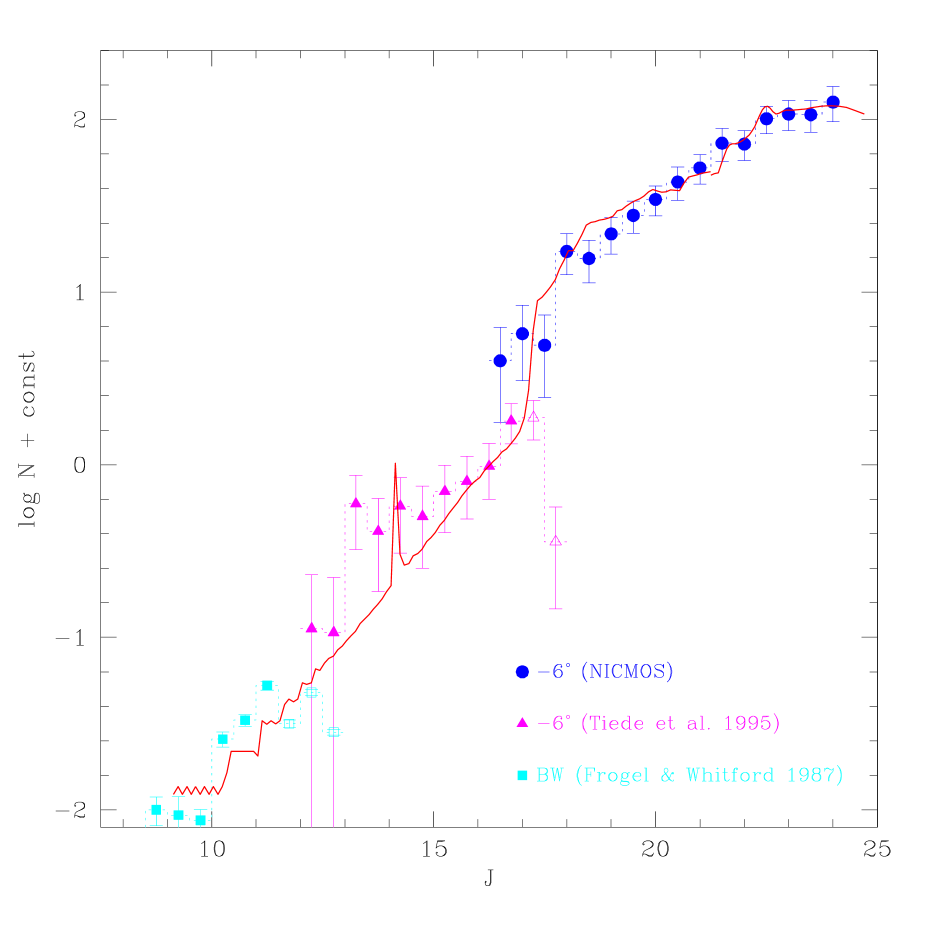
Figure 10: The LF shown in Fig. 4 is extended to bright magnitudes using the LF from Tiede et al. (1995). The brightest stars (filled squares) are taken from the wide-field survey of M giants in Baade’s Window (Frogel & Whitford 1987). Filled symbols show complete counts, while open symbols refer to counts affected by but not corrected for incompleteness. The solid line is the theoretical LF for a 10 Gyr, solar metallicity population, with IMF slope $\alpha=-1.33$ (see text). Note that the observed peak at $J\sim 13.5$ is the red clump of the HB stars, not included in the models, while the sharp peak in the theoretical LF at $J=14.15$ is the RGB bump.

8.2 Expected vs Observed Number of Stars

Having determined the actual slope of the IMF, we are now in a position to check the theoretical prediction concerning the number of MS stars in the observed field:

$$N\simeq\int_{0.15}^{1}\Psi(M)dM=A\int_{0.15}^{1}M^{-1.33}dM$$ (1)

where $A\simeq 1.2L_{\rm T}$ (Renzini 1998). From an optical CMD (Zoccali et al. 1999) referring to a field of $\sim 66$ arcmin² and using the distance and reddening adopted in the present paper, we determine an average surface brightness of the $-6^{\circ}$ field of 0.55 $\hbox{$L_{\odot}$}_{\rm V}\,\rm arcsec^{-2}$. Correcting for the disk contamination leaves an average surface brightness of the bulge alone of 0.35 $\hbox{$L_{\odot}$}_{\rm V}\,\rm arcsec^{-2}$. Hence, the total luminosity sampled by our 506 arcsec² field is $\sim 177\,\hbox{$L_{\odot}$}_{\rm V}$, or $L_{\rm T}=283\hbox{$L_{\odot}$}_{\rm Bol}$. Correspondingly, the number of stars in the $0.15-1\,\hbox{$M_{\odot}$}$ range is given by:

$$N\simeq 1.2\times 283\int_{0.15}^{1}M^{-1.33}dM=898\quad{\rm stars}$$ (2)

which compares well to the 820 stars observed.

8.3 The $M/L$ Ratio of the Galactic Bulge

By integrating the LF shown in Figure 10 we determine the total $J$ band luminosity sampled by a 506 arcsec² field to be $L_{J}=688.5L_{J\odot}$. Note that the stellar population sampled by our NIC2 field would not be representative of the entire bulge, being very small, and chosen to be in a region lacking very bright stars. However, the bright part of the LF was derived using stars in a field 8 times wider, and therefore we can trust the total luminosity calculated above as representative of the average surface brightness of the bulge at $b=-6^{\circ}$.

The total bulge mass in stars included in our 506 arcsec² field corresponds to the sum of the mass of the detected stars, plus the mass of M dwarfs and brown dwarfs with $M<0.15M_{\odot}$, plus the mass of white dwarfs, neutron stars, and black hole remnants, the end products of now defunct stars with $M{\mathrel{\mathchoice{\lower 2.9pt\vbox{\halign{$\m@th\displaystyle\hfil#\hfil$\cr>\crcr\sim\crcr}}}{\lower 2.9pt\vbox{\halign{$\m@th\textstyle\hfil#\hfil$\cr>\crcr\sim\crcr}}}{\lower 2.9pt\vbox{\halign{$\m@th\scriptstyle\hfil#\hfil$\cr>\crcr\sim\crcr}}}{\lower 2.9pt\vbox{\halign{$\m@th\scriptscriptstyle\hfil#\hfil$\cr>\crcr\sim\crcr}}}}}1\,\hbox{$M_{\odot}$}$.

We estimate the total mass in our field as follows. First, we simply sum the masses of the stars actually observed in the field (corrected for incompleteness and disk contamination) and obtain $317M_{\odot}$. By extrapolating the $\alpha=-1.33$ IMF from $M=0.15M_{\odot}$ all the way down to zero mass, we obtain $123.5M_{\odot}$ of unseen dwarfs, thus totaling $440.5M_{\odot}$ in living stars and brown dwarfs. To account for the remnants we need to adopt an initial mass-final mass relation. We used the semi-empirical relation proposed by Renzini & Ciotti (1993), with white dwarf remnants of mass $M_{\rm WD}=0.48+0.077\,M_{\rm i}$ for initial masses $M_{\rm i}\leq 8\,\hbox{$M_{\odot}$}$, neutron star remnants of $1.4\,\hbox{$M_{\odot}$}$ for $8\leq M_{\rm i}\leq 40\,\hbox{$M_{\odot}$}$, and black holes remnants of mass $0.5\,M_{\rm i}$ for $M_{\rm i}>40\,\hbox{$M_{\odot}$}$. Since the present data do not give any constraint on the slope of the IMF for $M{\mathrel{\mathchoice{\lower 2.9pt\vbox{\halign{$\m@th\displaystyle\hfil#\hfil$\cr>\crcr\sim\crcr}}}{\lower 2.9pt\vbox{\halign{$\m@th\textstyle\hfil#\hfil$\cr>\crcr\sim\crcr}}}{\lower 2.9pt\vbox{\halign{$\m@th\scriptstyle\hfil#\hfil$\cr>\crcr\sim\crcr}}}{\lower 2.9pt\vbox{\halign{$\m@th\scriptscriptstyle\hfil#\hfil$\cr>\crcr\sim\crcr}}}}}1\,\hbox{$M_{\odot}$}$, we explore the effect on the total mass of various plausible assumptions:

• IMF #1: An IMF with slope $\alpha=-1.33$, like the one we observed, all the way to $100M_{\odot}$. This is perhaps an extreme possibility, since all the determinations of the IMF in this mass range give steeper values (see Scalo 1998 for a recent review), and even our own IMF may steepen for $M>0.5M_{\odot}$.

• IMF #2: An IMF with slope $\alpha=-1.33$ up to $M=1M_{\odot}$ and $\alpha=-2$ for $M>1M_{\odot}$. This is the most conservative assumption, since the IMF we observed is best fit with a slope $\alpha=-2$ for $M>0.5M_{\odot}$.

• IMF #3: An IMF with $\alpha=-1.33$ up to $M=1M_{\odot}$ and $\alpha=-2.35$ (Salpeter’s value) for $M>1M_{\odot}$.

• IMF #4: Finally, we consider an IMF with $\alpha=-1.33$ up to $M=1M_{\odot}$, Salpeter slope for $1<M/M_{\odot}<2$ and $\alpha=-2.7$ (Scalo 1986) for $M>2M_{\odot}$.

For each of these four choices, Table 3 gives the total mass in the 506 arcsec² field, as well as the contribution of white dwarfs, neutron stars, and black holes. Of course, the mass of the unseen dwarfs ($M<0.15\,\hbox{$M_{\odot}$}$) and detected MS dwarfs is the same for all the IMF options. Finally, the last column gives the corresponding $M/L_{\rm J}$ ratio.

Option 1 is clearly top heavy, with most of the bulge baryonic mass in 20-50 $M_{\odot}$ black holes. With option 2 one gets rid of most of black holes, and the mass-to-light ratio drops to near unity. Further steepening the IMF, such as in options 3 and 4, ceases to have a major effect on the mass-to-light ratio, while reducing to just a trace contribution the mass of relativistic remnants. As the microlensing statistics improves, microlensing experiments may eventually allow us to select the best among these (or other) options.

8.4 Gravitational microlensing

In this section we consider the implications of our bulge IMF for the interpretation of the microlensing events that have been observed in the direction of the Galactic bulge. Only about 50 of these events have been published so far (Udalski et al. 1994; Alcock et al. 1997), but by now at least ten times more events should have been detected. The initial results have generated two somewhat orthogonal puzzles. First, the distribution of event timescales $t_{\rm E}$ is peaked toward much lower values ($t_{\rm E}\sim 10\,$days) than would be expected if the bulge IMF were as flat as $\alpha=-0.56$, as reported by Gould et al. (1997) for the disk MF, but would be well explained by a power-law IMF with $\alpha\sim-2$ and cut off near the hydrogen-burning limit (Zhao et al. 1995; Han & Gould 1996). Lower-mass lenses produce events that on average are shorter ($t_{\rm E}\propto M^{1/2}$), so a steeper IMF gives rise to a $t_{\rm E}$ distribution skewed toward shorter timescales. The slope reported here ($\alpha\sim-1.33$) is apparently not quite steep enough, though correcting for binaries may steepen the slope by a few tenths. Moreover, it has been shown that many of the shorter events seen toward the bulge are “amplification biased” events of faint sources that are below the threshold of detection Han (1997). These are mistaken for events of much brighter sources in the same seeing disk in which they are detected, and so the observed timescale for the period of significant apparent magnification is much shorter than the actual event timescale. Thus, the combination of our steeper IMF and the amplification bias may well allow the bulge microlensing events to be explained by ordinary stars (perhaps with a smooth extension into the brown dwarf regime).

It is not worth trying here to expand further on the implications of the bulge IMF for the interpretation of microlensing experiments, given the very small number of published events compared to the huge number that will soon become available. It will then be possible to make a detailed comparison between the observed timescale distribution from a large, very clean sample and that predicted on the basis of the IMF reported here. As for the $M/L$ ratio, the $f(t_{\rm E})$ distribution will depend not only on the IMF of still living stars, but also on the number and mass of the dead remnants, white dwarfs, neutron stars, and black holes. Such a distribution could provide constraints on the bulge IMF at masses greater than the present turnoff ($M\sim M_{\odot}$), even to $\sim 8\,M_{\odot}$ and beyond (Gould 1999)

9 Conclusions

We have presented the results of stellar photometry on deep images obtained with NICMOS on board of HST. The data refer to a field in the Galactic bulge, at a projected distance from the Galactic center of $\sim 6^{\circ}$. From the $J$-band LF of the stars in the field we derive the IMF of the Galactic bulge with the aid of a theoretical mass-luminosity relation which provides an excellent fit to the empirical MLR. The IMF so obtained refers to the mass range from $\sim 1\,\hbox{$M_{\odot}$}$ down to $\sim 0.15\,\hbox{$M_{\odot}$}$, being therefore the deepest IMF so far obtained for a Galactic bulge. Nevertheless, this low-mass limit is still nearly a factor of $\sim 2$ above the hydrogen burning limit.

The IMF is well fit by a single slope power law with $\alpha=-1.33\pm 0.07$, therefore much flatter than Salpeter’s IMF with $\alpha=-2.35$. A two-slope IMF with $\alpha=-2.00\pm 0.23$ above $0.50\,M_{\odot}$ and $\alpha=-1.43\pm 0.13$ below gives a better fit, formally at the $3\,\sigma$ level. However, in view of the larger error bars in the upper mass range, and the evolutionary effect away from the zero-age MS, we prefer to quote the single-slope power law as our main conclusion. This result is robust within current uncertainties in the reddening, distance modulus of the Galactic center, disk and binary stars contamination, and average metallicity of the bulge stars.

For the mass range in common ($0.35\hbox{$M_{\odot}$}\,{\mathrel{\mathchoice{\lower 2.9pt\vbox{\halign{$\m@th\displaystyle\hfil#\hfil$\cr<\crcr\sim\crcr}}}{\lower 2.9pt\vbox{\halign{$\m@th\textstyle\hfil#\hfil$\cr<\crcr\sim\crcr}}}{\lower 2.9pt\vbox{\halign{$\m@th\scriptstyle\hfil#\hfil$\cr<\crcr\sim\crcr}}}{\lower 2.9pt\vbox{\halign{$\m@th\scriptscriptstyle\hfil#\hfil$\cr<\crcr\sim\crcr}}}}}M{\mathrel{\mathchoice{\lower 2.9pt\vbox{\halign{$\m@th\displaystyle\hfil#\hfil$\cr<\crcr\sim\crcr}}}{\lower 2.9pt\vbox{\halign{$\m@th\textstyle\hfil#\hfil$\cr<\crcr\sim\crcr}}}{\lower 2.9pt\vbox{\halign{$\m@th\scriptstyle\hfil#\hfil$\cr<\crcr\sim\crcr}}}{\lower 2.9pt\vbox{\halign{$\m@th\scriptscriptstyle\hfil#\hfil$\cr<\crcr\sim\crcr}}}}}1\hbox{$M_{\odot}$}$), the derived IMF is in very good agreement with the bulge IMF obtained from optical observations with WFPC2 by Holtzman et al. (1998). Our bulge IMF, however, is appreciably steeper than the low mass IMF for the solar neighborhood found in two recent determinations, which give slopes of $\alpha=-0.8$ (Reid & Gizis 1997) and $\alpha=-0.54$ (Gould et al. 1997). However, the present bulge IMF is virtually identical to yet other determinations of the solar neighborhood IMF (Kroupa et al. 1993, Reid et al. 1999), and an assessment as to whether bulge and disk IMFs are the same or not will require an understanding the origin of the large discrepancies among the various determinations of the disk IMF.

We have also compared the bulge IMF with the present day MF of some Galactic globular clusters with different metallicities and affected to various degrees by dynamical processes. In all clusters the MF is flatter than that of the bulge, but it appears to be closer to the bulge IMF in those clusters that are less affected by dynamical processes. This suggests little or no dependence of the IMF on metallicity for old systems.

One major issue concerns the amount of bulge mass that is locked in unseen dwarfs. There is no hint for the IMF slope to change towards the lower mass limit ($0.15\,\hbox{$M_{\odot}$}$) of the explored range. Assuming the slope can be extrapolated all the way to mass zero, gives a total mass of brown dwarfs ($0<M<0.08\,\hbox{$M_{\odot}$}$) in the NIC2 field of $81\,\hbox{$M_{\odot}$}$, i.e., $<14\%$ of the total stellar mass in the field (c.f. Table 3). We note that some support for this extrapolation comes from the local density of L dwarfs (Reid et al. 1999). With all stars making up to $\sim 10\%$ of the total baryonic mass of the universe, this result suggests that brown dwarfs may represent not more than $1.4\%$, i.e. a minor fraction, of the baryonic mass of the universe.

Finally, we have estimated the $M/L_{J}$ mass to light ratio of the bulge to be very close to unity ($\sim 0.9\pm 0.1$) for reasonable assumptions of the IMF slope outside the directly explored range.

Table 1: The Luminosity Function

$J$	$N$	$N_{c}$	$\sigma$	Disk frac.
16.5	5	5	2	0.20
17.0	7	7	3	0.18
17.5	6	6	2	0.18
18.0	20	18	4	0.14
18.5	18	19	4	0.13
19.0	25	26	5	0.13
19.5	32	32	6	0.13
20.0	38	40	6	0.13
20.5	45	50	10	0.12
21.0	54	60	10	0.12
21.5	69	82	15	0.11
22.0	66	81	14	0.11
22.5	86	112	19	0.10
23.0	81	119	22	0.10
23.5	73	119	21	0.10
24.0	65	139	31	0.09
24.5	57	162	27	0.08

Table 2: Bright extension of the LF

$J$	$N$	$\sigma$	Disk frac.
8.750	0.010	0.002	0.00
9.250	0.009	0.003	0.00
9.750	0.009	0.003	0.00
10.250	0.026	0.004	0.00
10.750	0.033	0.004	0.00
11.250	0.052	0.005	0.00
11.750	0.032	0.005	0.00
12.250	0.112	0.116	0.00
12.750	0.112	0.113	0.05
13.250	0.661	0.268	0.10
13.750	0.447	0.223	0.08
14.250	0.661	0.263	0.13
14.750	0.661	0.246	0.24
15.250	1.000	0.290	0.30
15.750	1.230	0.310	0.35
16.250	1.660	0.343	0.41
16.750	2.754	0.464	0.35

Table 3: Bulge $M/L_{J}$ ratios

$\alpha$	$\alpha$	$\alpha$	$M_{TOT}$	$M_{WD}$	$M_{NS}$	$M_{BH}$	$M/L_{J}$
$M<1M_{\odot}$	$1<M/M_{\odot}<2$	$M>2M_{\odot}$
$-1.33$	$-1.33$	$-1.33$	3207	326	247	2213	4.7
$-1.33$	$-2.00$	$-2.00$	744	150	38	135	1.1
$-1.33$	$-2.35$	$-2.35$	601	133	15	32	0.9
$-1.33$	$-2.35$	$-2.70$	562	124	8	10	0.8

References

- (1) Alcock, C., et al. 1997, ApJ, 479, 119
- (2) Baraffe, I., Chabrier, G., Allard, F., & Hauschildt, P. H. 1997, A&A, 327, 1054
- (3) Bono, G., Caputo, F., Cassisi, S., Castellani, V., & Marconi, M. 1997, ApJ, 479, 279
- (4) Bouvier, J., Stauffer, J. R., Martín, E. L., Barrado y Navascués, D., Wallace, B., & Béjar, V. J. S. 1998, A&A, 336, 490
- (5) Cardelli, J. A., Clayton, G. C., & Mathis, J. S. 1989, ApJ, 345, 245
- (6) Cassisi, S., et al. 1999, in preparation
- (7) Dauphole, B., Geffert, M., Colin, J., Ducourant, C., Odenkirchen, M., & Tucholke, H.-J. 1996, A&A, 313, 119
- (8) De Marchi, G., Leibundgut, B., Paresce, F., & Pulone, L. 1999, A&A, 343, L9
- (9) Djorgovski, S. G. 1993, in: ASP Conf.Ser.50, Structure & Dynamics of Globular Clusters, Djorgovski S.G., Meylan G. (eds.), ASP, San Francisco, 373
- (10) Frogel, J. A., & Whitford, A. E. 1987, ApJ, 320, 199
- (11) Frogel, J. A., Terndrup, D. M., Blanco, V. M., & Whitford, A. E. 1990, ApJ, 353, 494.
- (12) Fugugita, M., Hogan, C. J., & Peebles, P. J. E. 1998, ApJ, 503, 518
- (13) Gould, A. 1999, ApJ, submitted, (astro-ph/9906472)
- (14) Gould, A., Bahcall, J. N., & Flynn, C. 1997, ApJ, 482, 913
- (15) Grillmair, C. J., Forbes, D. A., Brodie, J. P., & Elson, R. A. W. 1998, AJ, 117, 167
- (16) Han, C. 1997, ApJ, 484, 555
- (17) Han, C., & Gould, A. 1996, ApJ, 467, 540
- (18) Henry, T. J., & McCarthy, D. W.Jr. 1993, AJ, 106, 773
- (19) Hillenbrand, L. A. 1997, AJ, 113, 1733
- (20) Holtzman, J. A., Watson, A. M., Baum, W. A., Grillmair, C. J., Groth, E. J., Light, R. M., Lynds, R., & O’Neil, E. J.Jr. 1998, AJ, 115, 1946
- (21) Kent, S. M. 1992, ApJ, 387, 181
- (22) King, I. R., & Anderson, J., Cool, A. M., & Piotto, G. 1998, ApJ, 492, L37
- (23) Kroupa, P., Tout, C. A., & Gilmore, G. 1993, MNRAS, 262, 545
- (24) Larson, R. B. 1998, MNRAS, 301, 569
- (25) Luhman, K. L., Rieke, G. H., Lada, C. J., & Lada, E. A. 1998, ApJ, 508, 347
- (26) Maraston, C. 1998, MNRAS, 300, 872
- (27) Mc William, A., & Rich, R. M. 1994, ApJS, 91, 749
- (28) Miller, G. E., & Scalo, J. M. 1979, ApJS, 41, 513
- (29) Ortolani, S., Renzini, A., Gilmozzi, R., Marconi, G., Barbuy, B., Bica, E., & Rich, R. M. 1995, Nature, 377, 701
- (30) Piotto, G., Cool A. M., & King I. R. 1997, AJ, 113, 1345
- (31) Piotto, G., & Zoccali, M. 1999, A&A, 345, 485
- (32) Pulone, L., De Marchi, G., Paresce, F., & Allard, F. 1998, ApJ, 492, L41
- (33) Reid, I. N., & Gizis, J. E. 1997, AJ, 113, 2246
- (34) Reid, I. N., et al. 1999, ApJ, in press, (astro-ph/9905170)
- (35) Reid, M. 1993, ARA&A, 31, 345
- (36) Renzini, A., & Ciotti, L. 1993, ApJ, 416, L49
- (37) Renzini, A. 1998, AJ, 115, 2459
- (38) Renzini, A. 1999, in: When and How do Bulges Form and Evolve, Carollo C. M., Ferguson, H. C., Wyse, R. F. G. (eds.), Cambridge University Press, in press, (astro-ph/9902108)
- (39) Rich, R. M., Ortolani, S., Bica, E., & Barbuy, B. 1998, AJ, 116, 1295
- (40) Saumon, D., Bergeron, P., Lunine, J. I., Hubbard, W. B., & Burrows, A. 1994, ApJ, 424, 333
- (41) Scalo, J. 1998, in: ASP Conf.Ser.142, The Stellar Initial Mass Function, Gilmore G., Howell D. (eds.), San Francisco, 201
- (42) Scalo, J. 1999, in: The Birth of Galaxies, Guiderdoni B., et al. (eds.), Gif-sur-Yvette, in press
- (43) Stetson, P. B. 1987, PASP 99, 191
- (44) Stetson, P. B. 1994, PASP 106, 250
- (45) Stephens, A. W., Frogel, J. A., Renzini, A., Ortolani, S., Jablonka, P., Rich, R. M., & Davies, R. 1999, AJ, submitted
- (46) Tiede, G. P., Frogel, J. A., & Terndrup, D. M. 1995, AJ, 110, 2788
- (47) Udalski, A., Szymanski, M., Stanek, K. Z., Kaluzny, J., Kubiak, M., Mateo, M., Krzeminski, W., Paczynski, B., & Venkat, R. 1994, Acta Astron., 44, 165
- (48) Vesperini, E., & Heggie, D. C. 1997, MNRAS, 289, 898
- (49) Whitford, A. E. 1978, ApJ, 226, 777
- (50) Yan, L., Mc Carthy, P. J., Storrie-Lombardi, L. J., & Weymann, R. 1998, ApJ, 503, L19
- (51) Zhao, H. S., Spergel, D., & Rich, R. M. 1995, ApJ,440,L13
- (52) Zoccali, M., et al. 1999, in preparation