A search for variability in brown dwarfs and L dwarfs

Abstract

We have undertaken a differential photometric I band search for variability in three Pleiades brown dwarfs and three very low mass field L dwarfs. Analysis of the resultant time series for the Pleiades brown dwarfs (Teide 1, Calar 3, Roque 11) gives no evidence for variability (above 99% confidence) greater than 0.05 mags in any of these objects on timescales between 25 minutes and 27 hours. Time series of two of the L dwarfs, 2MASSW J0913032+184150 and 2MASSW J1146345+223053, are also consistent with no intrinsic variability (no significant variability above 0.07 mags for 30 mins $<\tau<$ 126 hours, and above 0.025 mags for 30 mins $<\tau<$ 75 hours, for the two objects respectively). However, the L dwarf 2MASSW J1145572 +231730 shows evidence for variability of amplitude 0.04 magnitudes with a tentative period of about 7 hours. It is therefore interesting that Kirkpatrick et al. (kirkpatrick99 (1999)) report an H$\alpha$ emission line of 4.2Å equivalent width for this star: If our detection is confirmed as a rotation period, it would support the link between rotation and H$\alpha$ emission in very low mass stars.

1 Introduction

Brown dwarfs are of great interest to astronomers. According to one definition they can be considered to bridge the gap between the lowest mass stable-hydrogen-burning stars and the Jupiter-like planets which do not get hot enough to burn deuterium, the most easily “combusted” element. Based on this definition, current models place their mass in the range $\approx$ 0.015–0.075 $M_{\odot}$ (D’Antona & Mazzitelli dantona94 (1994); Burrows et al. burrows97 (1997)). However, for single objects mass is not a directly observable quantity, so brown dwarf status can only be conferred via secondary indicators. Models predict that brown dwarfs spend most of their lives cooling, and all but the youngest and most massive brown dwarfs have effective temperatures below about 2800 K. Of particular interest, therefore, are the recently discovered compact objects with atmospheres characteristic of very low temperatures (Kirkpatrick et al. kirkpatrick99 (1999)). Models of these objects suggest 1500 K $<T_{\rm eff}<$ 2000 K, and the newly introduced class L dwarfs has been suggested to emphasise the status of these objects as a low temperature continuation of the M dwarfs. We therefore expect many of them to be brown dwarfs.

The intrinsic properties of brown dwarfs and L dwarfs are of astrophysical interest, and the observations and models to date raise a number of important questions. For example, what is the nature of their atmospheres? At temperatures below about 2500 K, models predict that dust grains start to condense and appear in the atmosphere (e.g. Allard et al. allard97 (1997)). How does the angular momentum of these objects evolve? Knowledge of their rotation speeds as a function of age and mass will help address the problem of the formation and evolution of these objects. Do these objects have magnetic activity and chromospheres? In higher mass objects, dynamo models give a relationship between rotation speed and magnetic activity (as observed, for example, via H$\alpha$ emission). The measurement of rotation periods and variability amplitudes is important for addressing these questions.

To date there has been very little work on measuring variability in brown dwarfs and L dwarfs. Tinney & Tolley (tinney99 (1999)) provide some evidence for photometric variability in the M9 brown dwarf LP 944-20, but do not derive a period for what they suspect to be a rotational modulation. Based on spectroscopy, Tinney & Reid (tinney98 (1998)) report $v\sin i$ of about $28\pm 2$ kms^-1 for this object. Martín et al. (martin98 (1998)) give a $v\sin i$ of $13\pm 1$ kms^-1 for the M6 Pleiades brown dwarf Teide 2, and Martín et al. (martin97 (1997)) derive a $v\sin i$ of $20\pm 10$ kms^-1 for the L5 field brown dwarf DENIS-P J1228.2-1547.

Table 1: Properties of brown dwarf and L dwarf targets. All data for the 2MASS objects are from Kirkpatrick et al. (kirkpatrick99 (1999)). For these objects $I$ is their $I_{spec}$ value (magnitude evaluated from a flux-calibrated spectrum).

name	IAU name	$I$	SpT	H$\alpha$ EW	${Li\textsc{i}}\,\lambda$6708 EW
				Å	Å
2M0913	2MASSW J0913032+184150	19.07	L3	$<0.8$	$<1.0$
2M1145	2MASSW J1145572+231730	18.62	L1.5	4.2 $\pm$0.2	$<0.4$
2M1146	2MASSW J1146345+223053	17.62	L3	$\leq 0.3$	5.1$\pm$0.2
Roque 11a	RPL J034712+2428.5b	18.75b	M8a	5.8 $\pm$1.0a
Teide 1c	TPL J034718+2422.5b	18.80b	M8d	3.5–8.6e	1.0$\pm$0.2f
Calar 3f		18.73g	M9d	6.5f–10.2d $\pm$ 1.0	1.8$\pm$0.4f

^aZapatero Osorio et al. (1997a )

^bZapatero Osorio et al. (zap99 (1999))

^cRebolo et al. (rebolo95 (1995))

^dMartín et al. (martin96 (1996))

^eseveral values are given in the literature: 6.1 $\pm$ 1.0 (Rebolo et al. rebolo95 (1995));

4.5 $\pm$ 1.0 (Rebolo et al. rebolo96 (1996)); 3.5 $\pm$ 2.0, 3.7  $\pm$ 2.0, 8.6 $\pm$ 2.0 (Zapatero Osorio et al. 1997a )

^fRebolo et al. (rebolo96 (1996))

^gZapatero Osorio et al. (1997b )

In this paper we present the results of a search for variability in six very low mass (VLM) stars (Table 1). Three of these are Pleiades brown dwarfs. Two (Teide~1 and Calar~3) are confirmed brown dwarfs, based on their radial velocities and lithium detections. The third, Roque~11, is a probable brown dwarf and cluster member. The three other objects (2M0913, 2M1145 and 2M1146) are L dwarfs discovered by the 2MASS survey. One of these, 2M1146, is a brown dwarf based on the detection of lithium in its spectrum. The other two have no or very little lithium, so are probably either VLM stars (just above the hydrogen burning limit), or old high mass ($>0.065M_{\odot}$) brown dwarfs.

The most likely cause of variability would be rotational modulation of the emitted flux. In the case of the three L dwarfs, this could be due to inhomogenous dust or other clouds rotating across the unresolved stellar disk. In theory, a modulation could also be observed on the timescale of formation and dissipation of the clouds, although this may be longer than the few days duration of our search. For all objects, modulation could be caused by surface star spots induced by a magnetic field.

2 Observations and Processing

The project was carried out with the 2.2m telescope at Calar Alto, Spain, using CAFOS and the 1K$\times$1K TEK13c CCD detector. The observations were obtained over the six nights 08/09 January to 13/14 January 1999 (MJD 2451187.4266 to 2451192.7560). However, due to poor weather (including frequent fog and poor seeing) and various technical problems, less than half of the available time could be spent obtaining data. The observing procedure was to cycle around the science fields in turn, taking five minute exposures in the I band in each field (Teide~1 and Roque~11 could be observed in the same field). A number of other fields were included for calibration purposes. The spacing between observations of a given field was non-uniform, although was typically 15–30 minutes on a given night.

The CCD frames were processed using IRAF. To help remove fringing in the CCD, a night sky flat was constructed from a clipped combination of 31 frames of 15 different fields.

For each science field, reference stars were selected which satisfied the following conditions:

• have a near-Gaussian, near-circular PSF

• are bright, but never saturated

• are isolated from other objects

• are as near as possible to the science object.

The reference stars were not know a priori to lack variability. About ten reference stars were typically found in each field. Fluxes at a range of aperture sizes were then evaluated for each reference star and science star using the IRAF aperture photometry task phot. Sky subtraction assumed a single value for the sky across the extraction aperture.

During reduction, 2M1146 was suspected to be a binary on account of the shape of its PSF. This was confirmed by Kirkpatrick et al. (kirkpatrick99 (1999)) who report a background star of much earlier spectral type separated by $\approx 1^{\prime\prime}$ from 2M1146.

3 Time Series Analysis

Intrinsic variations in a science star were searched for by looking for changes in the differential magnitude of the science star, that is, changes in the magnitude of the science star relative to a number of reference stars. This makes the observations relatively insensitive to changes in atmospheric transparency during or between exposures. For this to be successful, we must be confident that the reference stars are insignificantly variable themselves. We therefore adopted the following procedure to test for variability in the reference stars. A reference star, $s$, is chosen, and the average flux of all other reference stars formed. The relative magnitude of $s$ is then evaluated with respect to this average. This is done at every epoch, producing a time series $m_{s,1},m_{s,2},\ldots,m_{s,t},\ldots$, from which the mean is subtracted so that $\sum_{t}m_{s,t}=0$. At each epoch the total uncertainty in the relative magnitude, $\epsilon_{s,t}$, is also estimated (see below). We then use a $\chi^{2}$ test to decide whether the scatter of these relative magnitudes is consistent with their measurement uncertainties, using the statistic

$$\chi^{2}_{s}=\sum_{t}\left(\frac{m_{s,t}}{\epsilon_{s,t}}\right)^{2}\ \ \ .$$ (1)

The null hypothesis for this test is that there is no variability in the time series. If ${\rm P}(\chi^{2}_{s})$ is the probability that the null hypothesis is true, then the larger $\chi^{2}_{s}$ the smaller ${\rm P}(\chi^{2}_{s})$. A star will fail the test (show evidence for variability) if ${\rm P}(\chi^{2}_{s})<0.01$, a 99% confidence interval. (This would correspond to 2.5$\sigma$ significance if the distribution were Gaussian.) $\chi^{2}_{s}$ is measured for every reference star, and if any fails the test, the star with the highest $\chi^{2}$ is rejected from the set of reference stars. This whole process (starting from forming the time series for each star) is iterated until all remaining reference stars pass the $\chi^{2}$ test. These then define the reference system from which to determine the relative magnitude time series of the science star.

The point of using more than one reference star to determine the time series for the science star is that it increases the photometric precision of the relative magnitudes. Furthermore, any small residual variability in any one reference star will have a smaller effect on the average.

The $\chi^{2}$ test is a good initial test for variability, as it is sensitive to any type of variability and not just periodic variations. However, for the test to be successful, the errors, $\epsilon_{s,t}$, must be accurately determined. Using photon statistics we can evaluate the “formal” errors in any magnitude determination. These are (1) photon arrival noise from the object, (2) photon arrival noise from the sky, and (3) imperfect determination of the subtracted sky level. There are, however, additional “informal” errors which need to be accounted for if we are not to overestimate $\chi^{2}$. The most important of these results from imperfect flat fielding. We have estimated (from the construction of different flats) the accuracy of the flat to be $0.5\%$, and have combined this in quadrature with the formal error sources to give $\epsilon_{s,t}$. Other informal error sources include (4) imperfect centering of the aperture and (5) PSF variations over the frame. These were minimised by using a sufficiently large aperture. To maximise the signal-to-noise ratio in aperture photometry, one usually chooses an aperture of size approximately equal to the HWHM (half-width at half-maximum) of the PSF (Howell howell89 (1989)). It is not necessary to get all of the light – or apply an aperture correction – with relative photometry, provided that in a given frame a single-sized aperture is used and all stars have the same PSF. When there are PSF variations (as was the case for our data), a larger aperture must be used. This reduces the contribution from the informal errors (4 & 5) at the expense of increasing the formal errors (1–3). Thus the threshold for variability detections in any science star will be at a higher magnitude limit – but more reliable – than when using a smaller aperture. We found that an aperture size of about $4\times$HWHM reduced the informal errors to well below the $0.5\%$ level. Yet other sources of error (such as imperfect charge transfer efficiency and nonlinearity of the CCD flux sensitivity) are also below this level.

After establishing reliable reference stars, the $\chi^{2}$ test was applied to the science star. If it failed this test (gave evidence for variability), the next stage was to determine whether there was evidence for this variability being periodic. For this purpose we evaluated the modified periodogram described by Scargle (scargle82 (1982)). In contrast to the classical periodogram, it can be shown that the modified periodogram is equivalent to a least-squares fit (in the time domain) of sinusoids to the data (Lomb lomb76 (1976)). Furthermore, the method allows a simple determination of the significance of any peak in the periodogram based on the known noise in the data. We consider a peak to be significant only at the 99% level (i.e. when the probability, $p$, that a peak is due to noise is $<0.01$). If a significant peak is found, the time series is phased to the detected period and examined to see if it shows cyclic variability.

4 Results

We now have four criteria which the data must satisfy before a science star is flagged as showing evidence for periodic variations:

1. the science star has a significant $\chi^{2}_{s}$ value
   (${\rm P}(\chi^{2}_{s})<0.01$)

2. the time series looks plausible

3. the science star shows a significant ($p<0.01$) peak in the periodogram

4. the phased light curve at the detected period looks reasonable.

These tests were applied to the six science stars in Table 1. All except 2M1145 failed at least one. From the results of the $\chi^{2}$ test we can set approximate limits to the amount and timescale of intrinsic variability in these five stars at the epoch of the observations (Table 2). For each star in this table (except 2M1145) there is no significant evidence (i.e. ${\rm P}(\chi^{2}_{s})$ is $>$ 0.01) for variability above $I_{\rm lim}$ on the timescale shown. (This is not the same as saying that we are 99% confident that there is no variability above $I_{\rm lim}$. Moreover, larger variability on timescales to which we were not sensitive could be present.) Strictly, it is only possible to put a single magnitude limit on a given range of periods if the uncertainties ($\epsilon_{s,t}$) are the same for all $t$. This is not the case for our data due to changes in atmospheric conditions. Rather than defining different amplitude limits for different periods, we simply give an approximate limit for all periods. The upper limit period shown is the longest time base in our data. The shortest period is a sort of Nyquist period for the time series, and is slightly more than twice the shortest separation between frames. We emphasise that these figures should not be viewed as strict magnitude/period sensitivity limits.

Table 2: Approximate upper limits on intrinsic I band variability. $I_{\rm lim}$ is defined as the scatter of the RMS (root mean squared) values in the relative magnitude time series that would have been required before we obtained significant (${\rm P}(\chi^{2}_{s})<0.01$) evidence for variability according to the $\chi^{2}$ test. For each star the search was sensitive to variations in approximately the range shown.

Star	$I_{\rm lim}$	period range
2M0913	0.070	30 mins to 126.2 hours
2M1145	0.035	30 mins to 74.8 hours
2M1146	0.025	30 mins to 74.8 hours
Roque 11	0.045	25 mins to 26.4 hours
Teide 1	0.050	25 mins to 26.4 hours
Calar 3	0.050	25 mins to 27.5 hours

The star 2M1145 passed all four tests for variability, and showed a significant ($p<10^{-4}$) peak in the periodogram at about 7 hours. The phased light curve is shown in Fig 1. To be sure that the detected period was not due to a reference star, we calculated the periodogram of the relative magnitudes of each reference star (relative to the other reference stars, as described above). No reference star showed any even marginally significant peak. Additional checks on the variability detection in 2M1145 were made by using only a subset of the good reference stars in the reference set, and using slightly different aperture sizes in the original photometry. In all cases significant variability was detected (according to the above four criteria) and the determined periods were the same to within 1%.

The RMS (root mean squared) scatter of the relative magnitudes in Fig 1 is 0.038 mags, and the amplitude of a least-squares fit sinusoid ($A\times\sin[wt+\phi]$) is 0.040 mags. This latter value may be a slight overestimate of the amplitude of intrinsic variability on account of noise: the larger the aperture, the more noise in each measurement, and so the more likely it is that a larger amplitude is observed. This does not mean, however, that the detection is just due to noise, as with a much larger aperture the time series does not meet the variability criteria described above. This problem with least-squares fitting could be overcome using more robust techniques, but we choose to acquire a more extensive data set before making an improved determination. Nonetheless, Fig 1 shows evidence of periodic variation beyond the size of the error bars.

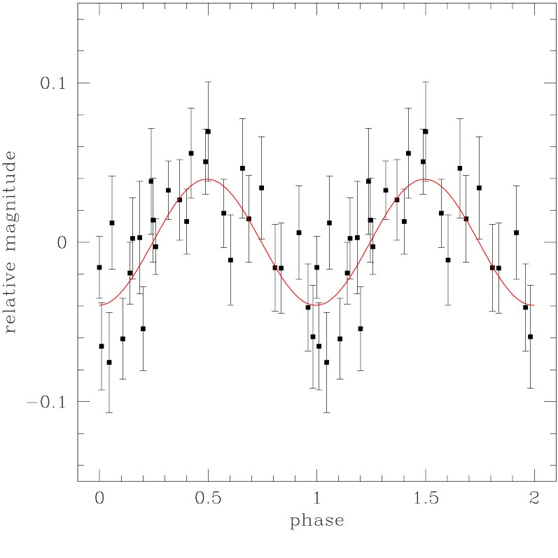
Figure 1: Light curve of the (zero mean) relative magnitude time series for the L dwarf 2M1145 phased at the detected period of 7.12 hours. Two (identical) periods are shown. The RMS scatter of the variations is 0.038 mags, and the amplitude of the overplotted least-squares fit sinusoid is 0.040 mags.

5 Discussion

The most plausible explanation for the observed periodic variation in 2M1145 is a rotational modulation of the emitted flux. Assuming a radius of $0.1M_{\odot}$ (Burrows et al. burrows97 (1997)), and rigid rotation, the period of 7.12 hours implies an equatorial rotation velocity of 17 kms^-1. This falls in the range of rotation speeds for 93 field M dwarfs measured by Delfosse et al. (delfosse98 (1998)) (all except one with $v\sin i$ in the range $<$ 2–32 kms^-1), but is smaller than the range for 9 Pleiades M5–M6.5 dwarfs observed by Oppenheimer et al. (oppenheimer97 (1997)) (37 $\leq v\sin i\leq$ 65 kms^-1). However, our data does not give unambiguous evidence for rotation at this speed. All we can say for certain is that we have evidence for periodic variability which is not present in the reference stars, and therefore is probably intrinsic to 2M1145. But given that we only have 28 points in our time series spread over several periods, confirmation of this period is required with a more extensive data set, preferably with smaller error bars and in more than one filter to provide somewhat independent measurements of the period. Observations should also be carried out over at least two (and preferably three or four) complete periods. We also stress that the period determination method assumes that the time series is stationary, in particular that the period and amplitude of the variations are constant: any evolution of surface features over the timescale of the observations would interfere with the interpretation of the periodogram. Additionally, multiple surface features may not give rise to a single sinusoidal modulation (and indeed, other peaks were present in the periodogram).

Given that the observations have only been carried out in a single filter, we can only speculate about the cause of the modulation in 2M1145. If its H$\alpha$ emission (Kirkpatrick et al. kirkpatrick99 (1999)) can be taken as evidence of magnetic activity, then the modulation could be the result of magnetically induced star spots. However, as we have only observed three L dwarfs we cannot draw any conclusions about the correlation between H$\alpha$ emission and rotation speed at the bottom of the main sequence, particularly as the amplitude limit on one of the targets (2M0913) is rather high. The observed modulations in 2M1145 could alternatively be the result of inhomogenous dust clouds rotating across the stellar disk. To distinguish between these two possibilities it will be necessary to re-observe in multiple filters (or with time resolved spectroscopy) to measure the change in $T_{\rm eff}$, and in filters sensitive to high dust opacity.

- (1) Allard F., Hauschildt P.H., Alexander D.R., Starrfield S., 1997, ARAA 35, 137
- (2) Burrows A., Marley M., Hubbard W.B., et al., 1997, ApJ 491, 856
- (3) D’Antona F., Mazzitelli I., 1994, ApJS 90, 467
- (4) Delfosse X., Forveille T., Perrier C., Mayor M., 1998, A&A 331, 581
- (5) Howell S.B., 1989, PASP 101, 616
- (6) Kirkpatrick J.D., Reid I.N., Liebert J., et al., 1999, ApJ, in press
- (7) Lomb N.R., 1976, Ap. Space Sci. 39, 447
- (8) Martín E.L., Rebolo R., Zapatero Osorio M.R., 1996, ApJ 469, 706
- (9) Martín E.L., Basri G., Delfosse X., Forveille T., 1997, A&A 327, L29
- (10) Martín E.L., Basri G., Gallegos J.E., et al., 1998, ApJ 499, L61
- (11) Press W.H., Teukolsky S.A., Vetterling W.T., Flannery B.P., 1992, Numerical Recipes, Cambridge University Press, second edition, p. 577
- (12) Oppenheimer B.R., Basri G., Nakajima T., Kulkarni S.R., 1997, AJ 113, 296
- (13) Rebolo R., Zapatero Osorio M.R., Martín E.L., 1995, Nat 377, 129
- (14) Rebolo R., Martín E.L., Basri G., Marcy G.W., Zapatero-Osorio M.R.,1996, ApJ 469, L53
- (15) Scargle J.D., 1982, ApJ 263, 835
- (16) Tinney C.G., Tolley A.J., 1999, MNRAS 304, 119
- (17) Tinney C.G., Reid I.N. 1998, MNRAS 301, 1031
- (18) Zapatero Osorio M.R., Rebolo R., Martín E.L., et al., 1997a, ApJ 491, L81
- (19) Zapatero Osorio M.R., Rebolo R., Martín E.L., 1997b, A&A 317, 164
- (20) Zapatero Osorio M.R., Rebolo R., Martín E.L., et al., 1999, A&AS 134, 537