Temperature Variation in the Cluster of Galaxies Abell 115 Studied with ASCA

Abstract

Abell 115 exhibits two distinct peaks in the surface brightness distribution. ASCA observation shows a significant temperature variation in this cluster, confirmed by a hardness ratio analysis and spectral fits. A linking region between main and sub clusters shows a high temperature compared with other regions. Two possibilities are examined as the cause of the temperature variation: cooling flows in the main cluster and a shock heating due to the collision of the subcluster into the main system. Spectral fits with cooling flow models to the main-cluster data show a mass-deposition rate less than $419M_{\odot}$ yr^-1. Temperatures in the main cluster, the linking region, and the subcluster are estimated by correcting for the effects of X-ray telescope response as $4.9^{+0.7}_{-0.6}$, $11^{+12}_{-4}$, and $5.2^{+1.4}_{-1.0}$ keV, respectively. The high temperature in the linking region implies that Abell 115 is indeed a merger system, with possible contribution from cooling flows on the temperature structure.

1 Introduction

Clusters of galaxies are the largest gravitationally bound system in the universe. They show us a large-scale distribution of matter in the universe and help us understand the structure and evolution of clusters themselves. X-ray images of the hot, intracluster medium (ICM) have been the most useful tool in determining cluster structures and morphology, since the gas traces the cluster gravitational potential generated by both visible and invisible matter.

Under a hierarchical structure formation scenario, substructures in the ICM are formed when interaction or merging occurs between subclusters. They disappear in a typical time scale (2 - 3 times the sound crossing time, Roettiger et al. 1996, 1997) of a few Gyr, therefore existence of a significant substructure strongly suggests that a cluster is still evolving. A variety of morphology in clusters has been revealed by the Einstein observatory. A definite scenario, however, does not exist concerning the detailed process of the evolution of clusters. For example, many clusters which have been recognized as typical relaxed systems, are now known to have complex temperature structures from ASCA (Honda et al. 1996). This clearly indicates that it is not enough to judge the evolutionary stage of clusters only from the surface brightness distribution, but we need to examine distributions of ICM temperature and metal abundance.

The cluster of galaxies Abell 115 (A115, Richness class = 3) is a fairly distant cluster ($z$ = 0.1971, Distance class = 6) and known in the literature to be characterized by a double peak X-ray surface brightness (Bautz-Morgan type = III, Abell et al. 1989). This morphology suggests that A115 is possibly in the process of a merger. The brightest galaxy in the center of the X-ray peak is associated with a radio source 3C 28.

The strong radio source 3C 28 was observed at 4.9 GHz with the Very Large Array (VLA) in 1984 April (Giovannini et al. 1987). High resolution and high sensitivity radio maps show two extended components located on northern and southern sides of the optical galaxy.

In the optical band, redshifts for 19 galaxies which are certainly associated with A115 were measured with the Kitt Peak National Observatory (KPNO) 4 meter telescope (R-band) (Beers et al. 1983). These plates reveal the presence of three primary clumps of galaxies. The two peaks in the X-ray surface brightness map correspond to the two concentrations in the galaxy distribution in the plates. No X-ray emission is, however, detected from the third clump which is $7^{\prime}$ east of the X-ray main peak by the Einstein observatory.

X-ray observations were performed with the Imaging Proportional Counter (IPC) in January 1979 (2.6 ksec) and the High Resolution Imager (HRI) in February 1981 (8.2 ksec) on board the Einstein Observatory. The IPC image revealed its X-ray surface brightness distribution with two clear enhancements (Forman et al. 1981). The ROSAT HRI observation was carried out in January and July 1994 (21 ksec and 30 ksec, respectively). The X-ray image in the archival data shows a similar double structure. The Einstein HRI observation showed no point-like source in the center of the main X-ray peak, and an upper limit to a point-source flux was estimated as $\lesssim 1.5\times 10^{-13}$ erg cm^-2 s^-1 (Feretti et al. 1984). Based on an image deprojection analysis of the Einstein imaging data, the main peak in A115 indicates a large cooling flow with a mass-deposition rate $\dot{M}=313^{+369}_{-186}M_{\odot}$ yr^-1 (White et al. 1997).

Previous X-ray observations, however, did not show detailed properties of the ICM in A115, except for its morphology. To examine dynamical state of the cluster, we need to look into structures of temperature and metal abundances with enough sensitivity. In this paper, we present results on the ICM properties of A115 obtained with ASCA. The large effective area covering up to 10 keV and the high spectroscopic resolution of ASCA (Tanaka et al. 1994) are particularly useful for the study of this cluster. Throughout this paper, we adopt $H_{0}=50$ km s^-1Mpc^-1 and $q_{0}=0$. At the distance of A115, $5^{\prime}$ corresponds to about 1.7 Mpc.

2 ASCA Observation

ASCA observation of A115 was carried out from 1994 Aug 5.96 to 7.02 (UT). The satellite carries four identical grazing-incidence X-Ray Telescopes (XRT, Serlemitsos et al. 1995, Tsusaka et al. 1995). Each XRT has approximately $3^{\prime}$ half power beam width. The point spread function (PSF) of the XRT has a cusp-shaped peak. This property allows us to partly resolve small-scale structures in clusters of galaxies. Two Solid-state Imaging Spectrometers (SIS0 and SIS1, Burke et al. 1991) and two Gas Imaging Spectrometers (GIS2 and GIS3, Ohashi et al. 1996, Makishima et al. 1996) are placed at the focal plane of the four XRTs. SIS has a Field Of View (FOV) of $22^{\prime}\times 22^{\prime}$ and covers an energy range 0.4 to 10 keV with a spectral resolution of 180 eV (FWHM) at 6 keV. GIS has a FOV of $50^{\prime}$ diameter and its energy range is from 0.7 to 10 keV. This instrument has a higher detection efficiency than SIS at the upper end of the energy band. These characteristics of ASCA allow us a sensitive study on the spatial structures of temperature and metal abundance in clusters of galaxies.

Throughout the observation of A115, GIS and SIS were operated in the normal PH mode and in the 1CCD Faint mode (FOV is $11^{\prime}\times 11^{\prime}$), respectively. We screened the data by requiring the cut-off rigidity to be $>6$ GeV $c^{-1}$ and $>8$ GeV $c^{-1}$, for GIS and SIS, respectively, and the target elevation angle above the earth rim to be $>5^{\circ}$. In the SIS data selection we used event grades of 0, 2, 3, and 4, and further required the elevation angle above the day earth rim to be $>25^{\circ}$. We also discarded data when the spacecraft was in high background regions such as the South Atlantic Anomaly (SAA). After removing data within $\sim 1.2$ hr just after the maneuver to A115, fluctuation of the pointing direction was kept within about $1^{\prime}$ in radius. We then added all of the available SIS data from the 2 sensor units (SIS 0 and SIS 1), regardless of the chip selection and data modes, and produced a single SIS spectrum after an appropriate gain correction. Similarly, data from GIS 2 and GIS 3 were summed into a single GIS spectrum.

Background (BGD) spectra were generated from blank-sky data in the public archive. Photons in the same detector region were accumulated for the source and for BGD. The blank sky data of SIS is taken only in 4CCD mode. Since the level of non X-ray background (NXB) is different between 4CCD and 1CCD modes, we adjusted it by normalizing with the detected intensity of Ni K_α and K_β lines, which are excited by the NXB flux.

Table 1 summarizes exposure times after the data selection, counting rates and fluxes, calculated for single temperature Raymond-Smith models (Raymond & Smith 1977) assuming $kT=5$ keV, for the whole cluster after the BGD subtraction.

3 Results

3.1 Image analysis

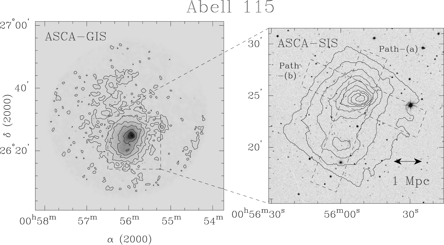
Figure 1: Left panel shows a greyscale GIS image of A115, superimposed on isointensity contours in a $60^{\prime}\times 60^{\prime}$ field centered on the field direction of GIS. Contour levels are logarithmic, showing 2.00, 4.15, 8.63, 17.9, 37.3, and 77.6 times the BGD level. Right panel also shows the Digitized Sky Survey image overlaid on a contour plot of the SIS image. The lowest contour level roughly corresponds to the edge of the field of view of SIS. Contour levels are 8.7, 11.6, 15.5, 20.6, 27.4, 36.5, 47.6, 64.7, and 86.3 times the BGD level. Two dashed rectangles indicate regions where data for the hardness ratio analysis are accumulated (see Figure 2). In both images, background images are not subtracted.

Figure 1 shows the surface brightness distribution of A115 observed with ASCA. These images are smoothed by a Gaussian function with $\sigma=0.^{\prime}32$. Left figure shows a greyscale ASCA GIS image, superposed on isointensity contours, in a $60^{\prime}\times 60^{\prime}$ field centered on the FOV. Right figure also shows the Digitized Sky Survey (DSS) image overlaid on the contours of ASCA SIS image. The lowest brightness contour roughly corresponds to the edge of the SIS FOV. Both contour levels are logarithmically evenly spaced and background image is not subtracted. In figure 1, the main peak (centered at R.A.[J2000] = $0^{h}55^{m}55^{s}$, Dec.[J2000] = $26^{\circ}24^{\prime}48^{\prime\prime}$) and the sub peak (centered at R.A.[J2000] = $0^{h}56^{m}04^{s}$, Dec.[J2000] = $26^{\circ}20^{\prime}33^{\prime\prime}$) are separated clearly, and no optical sources in the DSS image exist at the position of the X-ray main peak. We can confirm that A115 has an X-ray extent of more than $15^{\prime}$ ($\sim 5$ Mpc ) in diameter, and the surface brightness distribution obtained with ASCA is similar to that of Einstein IPC (Forman et al.  1981).

In the image analysis, we first fit the SIS radial profile with the $\beta$ model. The $\beta$ model surface brightness $I_{x}(r)$ at a projected radius $r$ varies as

$$I_{x}(r)=I_{0}\left\{1+\left(\frac{r}{R_{c}}\right)^{2}\right\}^{-3\beta+1/2},$$

where $R_{c}$ is the core radius and $I_{0}$ is the central brightness.

To obtain the $\beta$ model parameters which describe the X-ray emission from A115, we produced brightness distribution maps for various $\beta$ models and folded them with the PSF of the XRT. These simulated profiles were then compared with the SIS radial profile. We adjusted the parameters until the simulated profile gave a consistent fit to the observed profile. The parameter values for the main peak are $\beta=1.05^{+0.08}_{-0.06}$ and $R_{c}=1^{\prime}.22^{+0^{\prime}.29}_{-0^{\prime}.24}$, respectively, giving a $\chi^{2}_{\nu}$ value of 1.14 (d.o.f. = 55). We attempted to fit the radial profile for the sub peak. Due to the poor statistics, however, we could not constrain either $\beta$ or $R_{c}$ value. We thus fixed both $\beta$ and $R_{c}$ at the best-fit values for the main peak, and obtained normalization to be $0.33\pm 0.03$ times that of the main peak. The errors indicate 90% statistical errors for single parameter. With these $\beta$ model parameters, the observed brightness distribution is well reproduced.

3.2 Spatial variation of the hardness ratio

Figure 2 shows cross sections of the SIS and the GIS images in figure 1, along the path connecting the two emission peaks (Path-(a) in figure 2) and its vertical direction (Path-(b) in figure 2). The angular width of the data accumulation is $2.7^{\prime}$ for each path. The bottom panels show Hardness Ratios (H.R.) of the counting rates between the energy bands $2-10$ keV and $0.5-2$ keV. The dotted lines indicate corresponding temperatures for single temperature Raymond-Smith models. The H.R. for path-(a) shows the maximum between the main and the sub peaks, and becomes lower toward the main peak. If we fit this H.R. variation with a constant value, the $\chi^{2}_{\nu}$ value becomes 1.83 (d.o.f. = 6), indicating that a significant variation in the H.R. exists with a confidence level of more than 90% (Fig. 2; Path-(a)(SIS)). This is significant even if we allow the BGD level to vary by $\pm 10\%$. Therefore, the H.R. distributions in figure 2 indicate a real temperature variation in the ICM. The corresponding temperatures are $6\sim 8$ keV at the sub peak and 4 keV in the main cluster, respectively, if we assume the single temperature thermal emission.

The H.R. along the path-(b) is low near the main peak, similarly to that in the path-(a). Thus the central region of the cluster main peak may have a lower temperature than the outer regions. Because of the limited statistics, however, we can not definitely conclude from these results whether there exists an additional cool component such as the cooling flows suggested from the Einstein deprojection analysis (White et al. 1997).

3.3 Spectral analysis

Following the hardness ratio analysis, we investigate the variation of energy spectrum over the entire cluster. The pulse-height spectra are accumulated in 3 circular regions with a radius of $2^{\prime}$ or $3^{\prime}$. One centered on the main peak (northeast direction, R.A. = $0^{h}55^{m}55^{s}$, Dec. = $26^{\circ}24^{\prime}48^{\prime\prime}$, hereafter region A), one at the sub peak (south direction, R.A. = $0^{h}56^{m}04^{s}$, Dec. = $26^{\circ}20^{\prime}33^{\prime\prime}$, hereafter region C) , and one in an intermediate point between the two peaks (center of A115, R.A. = $0^{h}56^{m}03^{s}$, Dec. = $26^{\circ}23^{\prime}01^{\prime\prime}$, hereafter region B). As for the GIS data, larger integration radii of $5^{\prime}$ and $10^{\prime}$ centered on the main peak are also used. Figure 3 shows these integration regions overlaid on the GIS image.

In calculating the response function for the spectral fit, we assume that the surface brightness of the cluster is described by a double $\beta$ model as derived in section 3.1. The parameters are $\beta=1.05,R_{c}=1^{\prime}.22$, and the ratio of normalization between the 2 peaks = 1 : 0.33. This response also assumes that the cluster is isothermal. This assumption differs from the actual case, but it enables us to perform spectral fits separately in individual regions and gives approximate temperatures (see Honda et al. 1996). This method enables us to detect temperature variations in clusters, as already demonstrated for the Coma cluster (Honda et al. 1996, Kikuchi et al. 1998).

Figure 4 shows the observed GIS and SIS spectra for the on-source and the background data before subtracting the background. The background (CXB + NXB) level is less than 10% of the observed flux. Table 2 summarizes the number of photons in each integration region.

Figure 5 shows results of the spectral fit. Table 3 summarizes the spectral parameters for each integration region. The spectral fits are performed in the energy band 0.7 - 10 keV and 0.8 - 10 keV for SIS and GIS, respectively. Raymond-Smith and power-law models at a redshift $z=0.1971$ are assumed. Except for the region C which have very poor statistics, the power-law models are excluded. The best-fit galactic column densities turn out to be roughly 50% larger than the published value of $5.1\times 10^{20}$ cm^-2 (Stark et al. 1992). This is partly due to the uncertainty in the SIS response in the low energy band, and has no significant influence on other spectral parameters. For the integration regions A, B, and C, the BGD contributions are 7%, 9%, and 11% in a radius of $2^{\prime}$, respectively. The derived ICM temperature in each region varies by about 0.1 keV when the BGD normalization is varied by $\pm 10\%$. Uncertainty in the BGD level do have some effect on the energy response function through the change of the $\beta$ model parameters. Its effect on the temperature is, however, 0.05 keV or less for all regions.

The temperature for a region with $3^{\prime}$ radius is higher than that with $2^{\prime}$ for the regions A (main peak) and C (sub peak). On the other hand, integration over a $2^{\prime}$ radius indicates higher temperature than $3^{\prime}$ radius in the region B (linking region). This implies that the temperature takes the maximum value somewhere between the main and the sub peaks, and decreases toward each X-ray peak. This feature is consistent with the result of the H.R. analysis shown in figure 2.

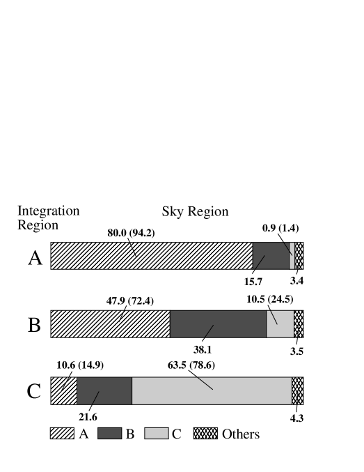
Figure 7: Fractions for the origins of photons detected in each integration region with $2^{\prime}$ radius (SIS data). Because of the tail of the point spread function, photons in each integration region are contaminated by those originating from the other sky regions. The three integration regions overlap with each other, and the numbers indicate the fractions when photons from the overlapped region are assigned as the region B. In round brackets, we also indicate the values when the data in the overlapping regions are assigned to either A or B.

More than half of the photons falling in region B ( $r=2^{\prime},kT=6.25$ keV) comes from region A ( $r=2^{\prime},kT=4.85$ keV) (figure 7, section 4.2), and the fraction of photons originating from the corresponding sky region is only 40%. The fact that the spectral fit for the region B data gives the highest temperature ($\sim 6$ keV) indicates that the true temperature in this region is even higher.

4 Origin of the temperature variation

Both the H.R. variation shown in figure 2 and the spectral analysis in section 3.3 indicate that the ICM temperature is high in the linking region between the main and the sub peaks. We will look into the possible processes which can cause the observed temperature variation along 2 broad scenarios: a cooling flow in the main cluster and a shock heating caused by a subcluster merger.

4.1 Cooling flows

If the center of the main peak has an intense cool component (cooling flows), then only the outer regions show the virial temperature of the cluster. The angular response of the XRT would cause the the cool component spread out in the detector plane over a few arcminutes. The H.R. profile in figure 2 in fact indicates that the central $3^{\prime}-4^{\prime}$ of the main peak has a soft spectrum, although the SIS profile along path-(a) is asymmetric around the main peak.

The Einstein observation showed that the main peak of A115 had the large mass-flow rate $\dot{M}=313^{+369}_{-186}M_{\odot}$ yr^-1 (White et al. 1997). The X-ray luminosity of the cooling flow with this mass-flow rate is estimated to be

$$L_{\rm cool}\simeq 7.9\times 10^{43}\left(\frac{kT_{\rm cool}}{1\ {\rm[keV]}}\right)\left(\frac{\dot{M}}{313\ [M_{\odot}{\rm yr}^{-1}]}\right)\ {\rm[erg\ s}^{-1}],$$

where $kT_{\rm cool}$ is an assumed temperature of the cool component. At the distance of A115, the expected flux is $F_{\rm cool}\simeq 4.7\times 10^{-13}$ erg cm² s^-1.

If the cooling flow occurs within 100 kpc ($\simeq 0.3^{\prime}$) of the center of the main peak, $L_{\rm cool}$ contributes about 16% of the flux in the energy band 0.5 - 10 keV in the region A with $r=2^{\prime}$. Table 4 summarizes results of spectral fits with various cooling flow models (Mushotzky & Szymkowiak, 1988). Because the mass-flow rate tightly couples with the galactic column density in this spectral fit, we fix it to the best fit value obtained in the previous spectral analysis (section 3.3).

The spectral fit was unable to constrain the slope parameter $s$ of the emission measure (EM) against temperature, when $s$ was a free parameter. We examined the spectrum by fixing the $s$ values between $-0.5$ and $+0.7$. This range corresponds to the 90% error when the mass-flow rate is set to $313M_{\odot}$ yr^-1 and includes the best-fit values ($s\sim 0.7$) for many other clusters reported by Mushotzky & Szymkowiak (1988). As shown in table 4 , the observed spectra can be fitted with a cooling flow model with the mass-flow rate reported by Einstein. In this case, the ICM temperature in region A becomes $5.5\sim 6.5$ keV, which is consistent with that in region B measured within $r=2^{\prime}$. This result indicates that we can interpret the temperature variation in A115 in terms of the cooling flow picture; i.e. the virial temperature in the main peak is in reality $\sim 6$ keV, which is suppressed in the ASCA data due to the presence of a cooling flow, and other regions in the cluster are filled with this $\sim 6$ keV ICM. We can then estimate confidence limits for the mass-flow rate based on the ASCA spectra for various fixed values of $s$. An upper limit for $\dot{M}$ is obtained as $419M_{\odot}$ yr^-1 in the case of $s=0.58$, which is lower than the limit set by the Einstein IPC (White et al. 1997).

We then calculated the expected H.R. profile assuming the cooling flow rate of $\dot{M}=313M_{\odot}$ yr^-1 in the main peak. Assuming that the main ICM has a temperature of 6 keV with the spatial extent as obtained in section 3.1 and the cool 1 keV component with an extent of 100 kpc ($\simeq 0.3^{\prime}$), the SIS image has been simulated because it has better spatial resolution than the GIS. Figure 6 shows the calculated profile overlaid on the H.R. data (Path-(a)(SIS) in figure 2). The cool region has a radius of about $3^{\prime}$ due to the PSF of the telescope. $\chi^{2}_{\nu}$ value for the simulated profile with the actual data is 1.0 (d.o.f. = 14), and the two profiles look similar with each other. Therefore, the cooling flow reported by the Einstein observation can account for the spatial variation of the temperature in A115.

4.2 Merger

The spectral fit of the main peak data (region A, $R=2^{\prime}$) with a cooling flow model showed the best-fit mass-flow rate to be $89M_{\odot}$ yr^-1, which is much smaller than the Einstein result. The ASCA spectrum is represented very well by the single temperature Raymond-Smith model (table 4). Regarding the fact that the highest temperature appears at the linking region between the main and the sub peaks, we should also interpret this feature in terms of shock heating due to a collision of the two subclusters. In this section, we will estimate the correct temperatures in the 3 regions in the cluster.

Since the PSF of ASCA XRT has an extended tail and the integrated regions A, B, and C are not far apart, significant fraction of photons detected in each region is contaminated by those from other sky regions. Therefore, we first estimate fractions of photon origins for each integration region.

The surface brightness distribution of A115 is approximated by a double $\beta$ model with the parameters $\beta=1.05,R_{c}=1^{\prime}.22$, and the flux ratio of the 2 peaks is 0.33. We then calculate, using the ASCA simulator, an expected image when photons of this surface-brightness distribution go through the XRT and reach the detectors. We then trace back each photon to the original sky coordinate. Figure 7 shows fractions of photon origins for each integration region thus estimated. As shown in this figure, 94% and 79% of the photons collected in the regions A and C, respectively, come from corresponding sky regions. There is, therefore, little influence from surrounding sky regions on the spectral results described in section 3.3. On the other hand, region B data contain only 38% of the photons produced in the corresponding sky, and a high fraction of photons come from region A ($\sim 48\%$) and C ($\sim 11\%$). The measured temperature for region B is then roughly an weighted average of the values in regions A, B and C.

To obtain the true temperatures of the sky regions, influence from other sky regions needs to be subtracted. This can be done using a ray-tracing simulation. True temperatures are estimated for regions A, B and C within $r<2^{\prime}$ using the SIS data, which are less contaminated because of the better position resolution. The actual process is an iterative one as described below.

(a)

To obtain a better estimate of the temperature in region C, calculate a contaminating spectrum from region A to C using the XRT and SIS responses and assuming the temperature of region A to be 4.97 keV. Then subtract it from the observed SIS data for the region C, and evaluate the temperature with the spectral fit. Note that the contamination from region B to C is negligible.

(b)

Calculate a contaminating spectrum from the regions A ( $kT=4.97$ keV ) and C ( with the temperature determined in step (a) ) to B. Then subtract it from the observed spectrum B, and evaluate its temperature.

(c)

In the same way as in step (b), simulate the spectrum from the regions B and C to A. Subtract it from the observed spectrum A, and evaluate its temperature.

(d)

Repeat the process (a) through (c) until the changes of temperatures of all the regions become less than 0.01 keV.

We assumed that the surface brightness follows 2 $\beta$ models for the main and the sub peaks and calculated the response function for the spectral fit. The integration regions A, B, and C, all having a $2^{\prime}$ radius, overlap with each other, and we allocated these overlapping data into region B in the spectral analysis. Table 5 shows the corrected temperatures compared with those evaluated in the previous section, only for the SIS data. As a result, the realistic temperatures of the three sky regions become $kT_{A}=4.9^{+0.7}_{-0.6}$ keV (main peak), $kT_{B}=11^{+12}_{-4}$ keV (between both peaks), and $kT_{C}=5.2^{+1.4}_{-1.0}$ keV (sub peak), respectively. The errors are evaluated by fixing the temperatures in other regions at their best-fit values. If temperature $kT_{A}$ is varied within this error range, the $kT_{B}$ value changes by ${}^{+2.0}_{-1.5}$ keV.

This analysis shows that the temperature in region B is significantly higher than that in region A. As seen in table 5, the regions A and C maintain almost the same temperature as the previous values in section 3.3. In contrast, fairly large change of temperature occurs in B. As shown in figure 3, the edge of region B is close to the main and the sub peaks of the surface brightness which have lower temperatures, even taking $r=2^{\prime}$. If we were able to limit the data within $r=1^{\prime}$, the temperature in this region would have become even higher; although it is not feasible because of too large statistical errors. To conclude, we obtain a strong suggestion that the ICM temperature in region B is very high.

5 Discussion

ASCA observations of A115 have revealed significant temperature structures in the ICM. The H.R. variation along the path connecting the two intensity peaks (Figure 2 Path-(a)) indicates that the temperature between the main and the sub peak is the highest. The spectral analysis based on an approximated response confirms the same feature (section 3.3). The cooling flow reported by the Einstein observation in the main cluster can account for this temperature variation (section 4.1). The mass-flow rate is obtained as $89M_{\odot}$ yr^-1 with an upper limit of $419M_{\odot}$ yr^-1, whose values are smaller than $313^{+369}_{-186}M_{\odot}$ yr^-1 reported by Einstein. The shock heating triggered by the merging is another possible interpretation for this feature, as suggested by the cluster morphology (section 4.2).

In the case of Hydra A cluster, which has been recognized as a typical cooling flow cluster with a very large mass-flow rate ($\dot{M}\sim 600M_{\odot}$ yr^-1, David et al. 1990) from the Einstein data, ASCA observation indicated a mass-flow rate of only $\dot{M}\sim 60M_{\odot}$ yr^-1 (Ikebe et al. 1997). This is an order of magnitude smaller than the previous estimate. The spectral information in the harder energy band, covering the hot component emission, is necessary for the correct estimation of the cool component flux.

We can estimate the central gas density $n_{0}$ and the cooling time in the main cluster as follows. The density $n_{0}$ is evaluated by taking $L_{X}\sim 9.1\times 10^{44}$ erg s^-1 and a $\beta$ model gas distribution in a volume $V\sim 10$ Mpc³ in the within $r<2^{\prime}$ in region A. This gives $n_{0}\simeq 3.3\times 10^{-3}$ cm^-3: which is comparable to the Einstein IPC result by Forman et al. (1981) of $1.8\times 10^{-3}$ cm^-3, but considerably lower than that estimated by Feretti et al. (1984) from the Einstein HRI data ($n_{0}=4.7\times 10^{-2}$ cm^-3). We regard that the HRI result is rather weighted on the interstellar matter associated with 3C28 because of the very small core radius (35 kpc). Taking the central densities by ASCA, cooling time is estimated to be $1.7\times 10^{10}$ yr which is comparable to the Hubble time. Though we have some uncertainty in the central density and the volume of ICM, it seems difficult for the cooling flow with a high $\dot{M}$ to develop in the center of A115 (around the radio galaxy 3C28).

On the other hand, we find it also possible to interpret the high temperature region in terms of a collision between the two subclusters. After correcting for the effects of contaminating photons from outside of the integrated sky regions (section 4.2), we evaluated the temperatures in three regions with $2^{\prime}$ radius to be $kT_{A}=4.9^{+0.7}_{-0.6}$ keV, $kT_{B}=11^{+12}_{-4}$ keV, and $kT_{C}=5.2^{+1.4}_{-1.0}$ keV, respectively. Since systematic uncertainties in the BGD level and in the response have little influence on the estimated temperatures, it is certain that A115 has a significant temperature structure along the main to subcluster path. This cluster is, therefore, probably undergoing an early phase of a subcluster merger.

When the merging scenario is assumed, a relative colliding velocity $v_{col}$ of the subcluster necessary to heat up the ICM temperature $kT$ from $\sim 5$ keV to $\sim 11$ keV. We further assume that the two subclusters are to cause a head-on collision and that their kinetic energies are completely converted to thermal energy. Thus, necessary value of $v_{col}$ to result in a temperature rise of $k\Delta T=6$ keV is given by,

$$v_{col} = \left(\frac{3k\Delta T}{\mu m_{p}}\right)^{1/2}$$

$$\simeq 1700\quad[{\rm km\ s}^{-1}]$$

where $\mu$ is the mean molecular weight (0.6) in amu, and $m_{p}$ is the proton mass, respectively. Beers et al. (1983) calculated a velocity dispersion for 6 galaxies which were unambiguously associated with A115 based on their mapping observation in the R band, and obtained $\sigma_{r}\simeq 1200$ km s^-1. The resulting $\beta(=\mu m_{p}\sigma_{r}^{2}/(kT))$ for $kT_{B}\sim 11$ keV turns out to be $\sim 0.8$, which is reasonable. In the cooling flow picture, the temperature of the hot-phase gas is obtained to be $\sim 6$ keV, which results in a somewhat low $\beta$ value.

Taking, $L_{X}\sim 5.1\times 10^{44}$ erg s^-1 and $V\sim 9.8$ Mpc³, in the spherical region B with $2^{\prime}$ radius, we obtain the average gas density in this region to be $n_{B}\simeq 3.8\times 10^{-4}$ cm^-3. The cooling time of the ICM in this region is estimated as

$$t_{\rm cool}\simeq 2.2\times 10^{11}\ {\rm[yr]}\left(\frac{n_{B}}{3.8\times 10^{-4}\ [{\rm cm}^{-3}]}\right)^{-1}\left(\frac{kT_{B}}{11\ {\rm[keV]}}\right)^{1/2}.$$

Therefore, cooling is not important in the region B. As a result, heating due to the collision of subclusters would effectively raise the ICM temperature.

Above considerations suggest that the shock heating caused by a subcluster merger is more important than the cooling flows in creating the observed spatial variation of temperature. ASCA and ROSAT observations detect spatial temperature structures from several clusters which are likely to be caused by subcluster mergers. For example, it became clear with ASCA observations of the Coma cluster that there are a low temperature region ($\sim 5$ keV) in the northeast and a high temperature one ($\sim 12$ keV) in the southwest (Honda et al. 1996). This provides evidence of a merger in this cluster. Many other clusters show significant temperature structures, such as A3558 (Markevitch & Vikhlinin 1997), Triangulum Australis cluster (Markevitch et al. 1996a), A2319, A2163, A665 (Markevitch 1996b), A2256 (Briel & Henry 1994, Roettiger et al. 1995, Markevitch 1996b), A2163 (Markevitch et al. 1994, 1996c), and A754 (Henry & Briel 1995, Henriksen & Markevitch 1996).

We cannot sufficiently constrain metal abundance and its variation in this cluster because of poor statistics. The best-fit values of abundance in the spectral analysis are 0.2, 0.1 and 0.2 solar for the regions A, B and C, respectively. The region B shows a somewhat lower value. Since the abundance distribution probably reflects the local density of galaxies (Ezawa et al. 1997), it may be reasonable that the linking region with low galaxy density shows a low metallicity.

6 Conclusion

ASCA observations of the cluster of galaxies A115 have revealed significant temperature variation in the ICM for the first time. The hardness ratio (H.R.) profile shows that the linking region between the two X-ray peaks has the highest temperature, which is confirmed with the spectral analysis. To investigate the origin of this temperature variation, we have looked into two possible scenarios: cooling flows in the main cluster and a shock heating due to the collision of the subcluster.

The ASCA spectrum of the main cluster is consistent with a cooling flow model with the mass deposition rate lower than the Einstein result. Our upper limit on the mass-flow rate is $419M_{\odot}$ yr^-1. The simulated H.R. profile including the cooling flow ($313M_{\odot}$ yr^-1) can reproduce the H.R. profile around the main cluster. However, the cooling time in the center of the main cluster is estimated to be $t_{\rm cool}\sim 1.7\times 10^{10}$ yr, which is comparable to the Hubble time. The cooling flow may not be the dominant process causing the temperature variation in A115.

On the other hand, merger scenario can explain the high temperature region in terms of a collision between the two subclusters, as suggested from its morphology. Temperatures are estimated by correcting for the contaminating flux due to the PSF of the XRT as $\sim 5$ keV and $\sim 11$ keV, for subcluster centers and the linking region, respectively. Observed velocity dispersion of galaxies in A115 and the ICM temperature of 5 keV indicates $\beta_{\rm spec}$ to be $\sim 0.8$, which is within a reasonable range for clusters. Cooling time of the gas in the linking region is much longer than the Hubble time because of the low density. Based on these features, we conclude that heating due to the collision of the subcluster is probably the major cause of the temperature variation in A115. It is also likely that the presence of cooing flows in the main cluster makes the temperature distribution more complicated.

We thank anonymous referee for pointing out the possibility of cooling flows. We would like to express our thanks to the ASCA team and the ASCA_ANL, SimASCA, and SimARF software development team for constructing excellent frameworks for the analysis. We also thank F. Makino and S. Uno for valuable advice on the analysis method. R. S. acknowledges support from the Japan Society for the Promotion of Science for Young Scientists.

Table 1: ASCA observation of A115.

Detector	DP Mode	Exposure Timea	Counting Rateb	Flux(0.5-10keV)c
		[s]	[counts s-1]	[erg cm-2 s-1]
SIS-0			0.291
	Faint	32,000		(9.6 $\pm 0.4)\times 10^{-12}$
SIS-1			0.223
GIS-2			0.183
	PH nominal	33,100		(1.1 $\pm 0.1)\times 10^{-11}$
GIS-3			0.220
$a$ : Average for SIS0 and SIS1, and for GIS2 and GIS3.
$b$ : Integration regions are $11^{\prime}\times 11^{\prime}$ for SIS and 10′ radius for GIS.
$c$ : Assuming a single temperature Raymond-Smith model with a best fit temperature $kT$ = 5 keV ($z$ = 0.1971). The errors indicate 90% statistical ones.

Table 2: The number of photons in each integration region

Integration Radius	Counting Ratea [$\times$ 10-2 counts s-1]
$[$arcmin.](sensor)	Region A	Region B	Region C
2 (GIS)	4.98 (0.23)	3.73 (0.22)	2.83 (0.21)
2 (SIS)	8.89 (0.54)	6.61 (0.54)	4.50 (0.44)
3 (GIS)	8.31 (0.51)	8.16 (0.51)	5.29 (0.47)
3 (SIS)	14.6 (1.17)	14.6 (1.13)	9.54 (1.05)
5 (GIS)	14.9 (1.38)
10 (GIS)	25.5 (5.43)
a: Counting rates in round brackets indicate those of background data.

Table 3: The fitting parameters for each integration region. The GIS and SIS data are jointly fitted.

Integration	Integration	Spectral Model a
Region	Radius	Raymond & Smith
	[arcmin.]	$kT$[keV]	Abundance	$N_{H}$[$\times$ 1021cm-2]	$\chi^{2}/\nu$
A	2	4.85${}^{+0.45}_{-0.40}$	0.21${}^{+0.08}_{-0.08}$	0.91${}^{+0.28}_{-0.25}$	163.8/159
A	3	5.37${}^{+0.42}_{-0.39}$	0.15${}^{+0.07}_{-0.07}$	0.76${}^{+0.22}_{-0.21}$	194.0/159
A	5 ∗	5.64${}^{+0.68}_{-0.53}$	0.14${}^{+0.09}_{-0.08}$	0.66${}^{+0.46}_{-0.46}$	96.29/79
A	10 ∗	5.05${}^{+0.47}_{-0.43}$	0.28${}^{+0.09}_{-0.09}$	0.96${}^{+0.41}_{-0.41}$	88.86/79
B	2	6.25${}^{+0.93}_{-0.77}$	0.10${}^{+0.10}_{-0.10}$	0.84${}^{+0.37}_{-0.33}$	215.7/159
B	3	5.74${}^{+0.54}_{-0.42}$	0.13${}^{+0.07}_{-0.06}$	0.93${}^{+0.23}_{-0.23}$	192.1/159
C	2	5.08${}^{+0.71}_{-0.61}$	0.21${}^{+0.12}_{-0.12}$	1.32${}^{+0.44}_{-0.41}$	144.2/159
C	3	5.52${}^{+0.62}_{-0.52}$	0.21${}^{+0.09}_{-0.09}$	1.06${}^{+0.31}_{-0.31}$	159.6/159
$a$ : $N_{H}$ = free, redshift = 0.1971 (fixed). The errors indicate 90% statistical ones.
$*$ : Only GIS data are used because the regions are not covered with the SIS FOV.

Table 4: The results of spectral fit to inspecting the cooling flow in the region A within 2^′ radius . The GIS and SIS data are jointly used.

ICM			cool component
Raymond-Smith model			cooling flow model a
kT[keV]	Abundance		slope	mass-flow rate [M⊙]		$\chi^{2}/\nu$
4.85 ${}^{+0.45}_{-0.40}$	0.21 ${}^{+0.08}_{-0.08}$		—	—		163.8/159
5.45 ${}^{+0.39}_{-0.37}$	0.17 ${}^{+0.09}_{-0.09}$		$-$0.5 (fixed)	313 (fixed)		170.5/160
5.63 ${}^{+0.43}_{-0.42}$	0.18 ${}^{+0.09}_{-0.09}$		0.0 (fixed)	313 (fixed)		168.5/160
6.53 ${}^{+0.82}_{-0.70}$	0.19 ${}^{+0.09}_{-0.09}$		0.7 (fixed)	313 (fixed)		168.2/160
4.85 ${}^{+0.45}_{-0.29}$	0.21 ${}^{+0.08}_{-0.08}$		$-$0.5 (fixed)	$<$ 282		163.8/159
4.85 ${}^{+0.64}_{-0.29}$	0.21 ${}^{+0.09}_{-0.08}$		0.0 (fixed)	$<$ 362		163.8/159
5.00 ${}^{+0.95}_{-0.44}$	0.21 ${}^{+0.09}_{-0.08}$		0.58 (fixed)	89 ${}^{+330}_{-89}$		163.6/159
5.01 ${}^{+0.94}_{-0.45}$	0.21 ${}^{+0.07}_{-0.08}$		0.7 (fixed)	88 ${}^{+319}_{-88}$		163.6/159
$a$ : We adopt the model made by Mushotzky & Szymkowiak (1988). Low temperature is fixed with 0.1 keV, and high temperature is linked up with the temperature of ICM. Redshift and column density are also fixed with 0.1971 and galactic value, respectively. The errors indicate 90% statistical ones.

Table 5: The ICM temperature in each integration region using only SIS data, which have less contamination than the GIS data. The used responses are calculated assuming an isothermal ICM throughout the whole cluster (“Raw Values” in the table), and a non isothermal ICM which is corrected for the flux contamination due to the XRT (“Real Values” in the table), respectively.

		Temperature [keV]			Reference
		Region A	Region B	Region C	Section
Raw values		5.0${}^{+0.6}_{-0.6}$	6.8${}^{+1.6}_{-1.1}$	5.3${}^{+1.2}_{-0.9}$	3.3
Real Values		4.9${}^{+0.7}_{-0.6}$	11${}^{+12}_{-4}$	5.2${}^{+1.4}_{-1.0}$	4.2
NOTE : The errors indicate 90% statistical ones.

Figure 2: Intensity and hardness ratio profiles of A115 along 2 paths measured with GIS and SIS. Left and right panels are for path-(a) and path-(b) accumulated in a rectangular region having a width of $2.7^{\prime}$ (see figure 1). Top and bottom panels are for the GIS and the SIS data, and filled circles and crosses indicate raw and background data, respectively. The arrows also indicate the regions A, B, and C with $2^{\prime}$ radius each, which are used for the spectral analysis in section 3.3. Bottom diagram in each panel shows hardness ratio profile for counting rates between $2-10$ keV and $0.5-2$ keV. The dotted lines indicate corresponding temperatures for Raymond-Smith models (4.0, 6.0, and 8.0 keV).

Figure 3: Grey-scale plot of integration regions for the spectral analysis overlaid on the GIS image. Spectra in these seven integration regions are analyzed in section 3.3. The centers of the regions correspond to the main peak (region A), sub peak (region C) and the midpoint between the two peaks (region B), respectively. The circles with slid lines indicate radii of $2^{\prime}$ and $3^{\prime}$, and spectral analyses are carried out for GIS and SIS data. The broken circle with a radius of $5^{\prime}$ indicates a region for GIS spectral analysis.

Figure 4: Observed GIS and SIS spectra integrated in a radius of $3^{\prime}$. Left and right panels correspond to GIS and SIS, respectively. Top, middle, and bottom panels are for regions A, B, and C, respectively. Filled circles and crosses indicate raw and background spectra, and arrows show expected energy for a Fe K_α emission line.

Figure 5: The background subtracted GIS and SIS spectra fitted thermal models. The integrated radius is $3^{\prime}$. The layout is the same as that in figure 4. Filled circles, lines, and open circles indicate observed data, best-fit models, and residuals of the fit, respectively. We adopted single temperature Raymond-Smith models with a redshift $z=0.1971$.

Figure 6: The simulated H.R. profile assuming a cooling flow with $\dot{M}=313M_{\odot}$ yr^-1 exist in the main peak. Solid line indicates the simulation result and crosses show observed data.

References

- (1) Abell, G. O., Corwin, H. G., Olowin, R. P, 1989, ApJS, 70, 1
- (2) Beers, T. C., Huchra, J. P. and Geller, M. J., 1983, ApJ, 264, 356
- (3) Briel, U. G. & Henry, J. P.,1994, Nature, 372, 439
- (4) Burke, B. E., Mountain, R. W., Harrison, D. C., Bautz, M. W., Doty, J. P., Ricker, G. R., Daniels, P. J., 1991, IEEE Trans. ED-38, 1069
- (5) David, L. P., et al., 1990, ApJ, 356, 32
- (6) Ezawa, H., et al., 1997, ApJ, 490, L33
- (7) Feretti, L., Gioia, I. M., et al., 1984, A&A, 139, 50
- (8) Forman, W., et al., 1981, ApJ, 243, L133
- (9) Giovannini, G., Feretti, L. and Gregorini, L., 1987, A&AS 69, 171
- (10) Henriksen, M. J., & Markevitch, M. L., 1996, ApJ, 466, L79
- (11) Henry, J. P. & Briel, U. G., 1995, ApJ, 443, L9
- (12) Honda, H., et al., 1996, ApJ, 473, L71
- (13) Ikebe, Y., et al., 1997, ApJ, 481, 660
- (14) Kikuchi, K., et al., 1998, PASJ, Submitted
- (15) Makishima. K., et al., 1996, PASJ, 48, 171
- (16) Markevitch, M. et al., 1994, ApJ, 436, L71
- (17) Markevitch, M. et al., 1996a, ApJ, 472, L17
- (18) Markevitch, M., 1996b, ApJ, 465, L1
- (19) Markevitch, M. et al., 1996c, ApJ, 456, 437
- (20) Markevitch, M. & Vikhlinin, A. 1997, ApJ, 474, 84 1993, ARA&A, 31, 717
- (21) Mushotzky & Szymkowiak, “Cooling Flows in Clusters and Galaxies” ed. Fabian, 53, 1988
- (22) Ohashi, T., et al., 1996, PASJ, 46, 87
- (23) Raymond, J. C., & Smith, B. W., 1977, ApJS, 35, 419
- (24) Roettiger, K., et al., 1995, ApJ, 453, 634
- (25) Roettiger, K., et al., 1996, ApJ, 473, 651
- (26) Roettiger, K., et al., 1997, ApJS, 109, 307
- (27) Serlemitsos, P. J., Jalota, L., et al., 1995, PASJ, 47, 105
- (28) Stark A. A., et al., 1992, ApJS, 79, 77
- (29) Tanaka, Y., Inoue, H. & Holt, S. S., 1994, PASJ, 46, L37
- (30) Tsusaka, Y., Suzuki, H., et al., 1995, Appl. Opt., 34, 4848,
- (31) White, D. A., Jonse, C., and Forman, W., 1997, MNRAS, 292, 419