SPH simulations of magnetic fields in galaxy clusters

Abstract

We perform cosmological, hydrodynamic simulations of magnetic fields in galaxy clusters. The computational code combines the special-purpose hardware Grape for calculating gravitational interaction, and smooth-particle hydrodynamics for the gas component. We employ the usual MHD equations for the evolution of the magnetic field in an ideally conducting plasma. As a first application, we focus on the question what kind of initial magnetic fields yield final field configurations within clusters which are compatible with Faraday-rotation measurements. Our main results can be summarised as follows: (i) Initial magnetic field strengths are amplified by approximately three orders of magnitude in cluster cores, one order of magnitude above the expectation from spherical collapse. (ii) Vastly different initial field configurations (homogeneous or chaotic) yield results that cannot significantly be distinguished. (iii) Micro-Gauss fields and Faraday-rotation observations are well reproduced in our simulations starting from initial magnetic fields of $\sim 10^{-9}\,{\rm G}$ strength at redshift 15. Our results show that (i) shear flows in clusters are crucial for amplifying magnetic fields beyond simple compression, (ii) final field configurations in clusters are dominated by the cluster collapse rather than by the initial configuration, and (iii) initial magnetic fields of order $10^{-9}\,{\rm G}$ are required to match Faraday-rotation observations in real clusters.

1 Introduction

Magnetic fields in galaxy clusters are inferred from observations of diffuse radio haloes (Kronberg 1994), Faraday rotation (Vallee, MacLeod & Broten 1986, 1987), and recently also hard X-ray emission (Bagchi, Pislar & Lima Neto 1998). The diffuse radio emission comes from the entire clusters rather than from individual radio sources. It is typically unpolarised and has a power-law spectrum, indicative of synchrotron radiation from relativistic electrons with a power-law energy spectrum in a magnetic field. Since the magnetised intra-cluster plasma is birefringent, it gives rise to Faraday rotation, which is detectable through multi-frequency radio observations of polarised radio sources in or behind the clusters. Hard X-ray emission is due to CMB photons which are Compton-upscattered by the same relativistic electron population responsible for the synchrotron emission. Upper limits to the hard X-ray emission have previously been used to infer lower limits to the magnetic field strengths: Stronger fields require less electrons to produce the observed radio emission, and this electron population is less efficient in scattering CMB photons to X-ray energies. Even non-detections of hard X-ray emission (e.g. Rephaeli & Gruber 1988) have therefore been useful to infer that cluster-scale magnetic fields should at least be of order $1\,\mu{\rm G}$. Combined observations of hard X-ray emission and synchrotron haloes are most valuable. They allow to infer magnetic field strengths without further restrictive assumptions because they are based on the same relativistic electron population.

It is therefore evident that clusters of galaxies are pervaded by magnetic fields of $\sim\mu{\rm G}$ strength. Small-scale structure in the fields has been seen in high-resolution observations of extended radio sources (Dreher, Carilli & Perley 1987; Perley 1990; Taylor & Perley 1993; Feretti et al. 1995), and inferred from Faraday rotation measurements in conjunction with X-ray observations and inverse-Compton limits (Kim et al. 1990). Coherence of the observed Faraday rotation across large radio sources (Taylor & Perley 1993) demonstrates that there is at least a field component that is smooth on cluster scales. Very small-scale structure and steep gradients in the Faraday rotation measure (Dreher et al. 1987; Taylor, Barton & Ge 1994) may partially be due to Faraday rotation intrinsic to the sources or in cooling flows in cluster centres.

Various models have been proposed for the origin of cluster magnetic fields in individual galaxies (Rephaeli 1988; Ruzmaikin, Sokolov & Shukurov 1989). The basic argument behind such models is that the metal abundances in the intra-cluster plasma are comparable to solar values. The plasma therefore must have been substantially enriched by galactic winds which could at the same time have blown the galactic magnetic fields into intra-cluster space.

Magnification of galactic seed fields in turbulent dynamos driven by the motion of galaxies through the intra-cluster plasma appeared for some time as the most viable model (Ruzmaikin et al. 1989; Goldman & Rephaeli 1991). It has been shown recently (De Young 1992; Goldshmidt & Rephaeli 1993) that it is difficult for that process to create cluster-scale fields of the appropriate strengths, mainly because of the small turbulent velocities driven by galactic wakes, and because turbulent energy cascades to the dissipation scale more rapidly than the dynamo process could amplify the field. Field strengths of $0.1\,\mu{\rm G}$ seem to be the maximum achievable under idealised conditions, and typical correlation scales are of order the turbulent scale, $\sim 10\,{\rm kpc}$, and below.

It is clear that this dynamo mechanism occurs in galaxy clusters and produces small-scale structure in the cluster magnetic fields. Other processes have to be invoked as well in order to explain micro-Gauss fields on cluster scales.

We here address the question whether primordial magnetic fields of speculative origin, magnified in the collapse of cosmic material into galaxy clusters, can reproduce a number of observations, particularly Faraday-rotation measurements. Specifically, we ask what initial conditions we must require for the primordial fields in order to reproduce the statistics of rotation-measure observations. A compilation of available observations of this kind was published by Kim, Kronberg & Tribble (1991).

Measurements of Faraday rotation are made possible by the fact that synchrotron emission in an ordered magnetic field produces linearly polarised radiation, and therefore the emission of many observed radio sources is linearly polarised to some degree. The plane of polarisation is rotated when the radiation propagates through a magnetised plasma like the intra-cluster medium (ICM). Observing a background radio source through a galaxy cluster at different wavelengths, and measuring the position angle $\phi$ of the polarisation allows to determine the rotation measure,

$${\rm RM} = \Delta\phi\,\frac{\lambda_{1}^{2}\lambda_{2}^{2}}{\lambda_{2}^{2}-\lambda_{1}^{2}}=\frac{e^{3}}{2\pi m_{\rm e}^{2}\,c^{4}}\int n_{\rm e}B_{\parallel}{\rm d}l$$ (1)

$$= 812\,\frac{{\rm rad}}{{\rm m}^{2}}\,\int\frac{n_{\rm e}}{{\rm cm}^{-3}}\,\frac{B_{\parallel}}{\mu{\rm G}}\,\frac{{\rm d}l}{{\rm kpc}}\;.$$

It can have either sign, depending on the orientation of the magnetic field. Figure 1 shows all published rotation measures observed in radio sources seen through the Coma cluster (Kim et al. 1990). The observed Faraday rotation is averaged across the source or the telescope beam, whichever is smaller. Most of the sources used for Faraday-rotation measurements are QSOs or faint radio galaxies, whose size is negligible compared to the resolution of the simulations presented below. The number of RM values available per cluster depends on the number-density of background radio sources bright enough to measure polarisation. The noise level for reliable Faraday-rotation measurements is about $25-35\,\mu{\rm Jy}$ for several minutes of integration time at the VLA. The polarised flux should be about $300\,\mu{\rm Jy}$, i.e. the total flux should be about $10~{}mJy$ for a source polarised at the level of a few per cent. With a large amount of observation time one could reach about $20-40$ rotation measures per square degree (P.P. Kronberg, private communication). We note that Kim et al. (1990) had on average 4 background rotation measures per square degree for the Coma cluster.

Thanks to recent compilations (Kim et al. 1991; see also Goldshmidt & Rephaeli 1993) of large rotation-measure samples, the observational basis for our exercise now seems to be sufficiently firm.

The numerical method used rests upon the GrapeSPH code written and kindly provided by Matthias Steinmetz (Steinmetz 1996). The code combines the merely gravitational interaction of a dark-matter component with the hydrodynamics of a gaseous component. We supplement this code with the magneto-hydrodynamic equations to trace the evolution of the magnetic fields which are frozen into the motion of the gas because of its ideal electric conductivity. The latter assumptions precludes dynamo action in our simulations.

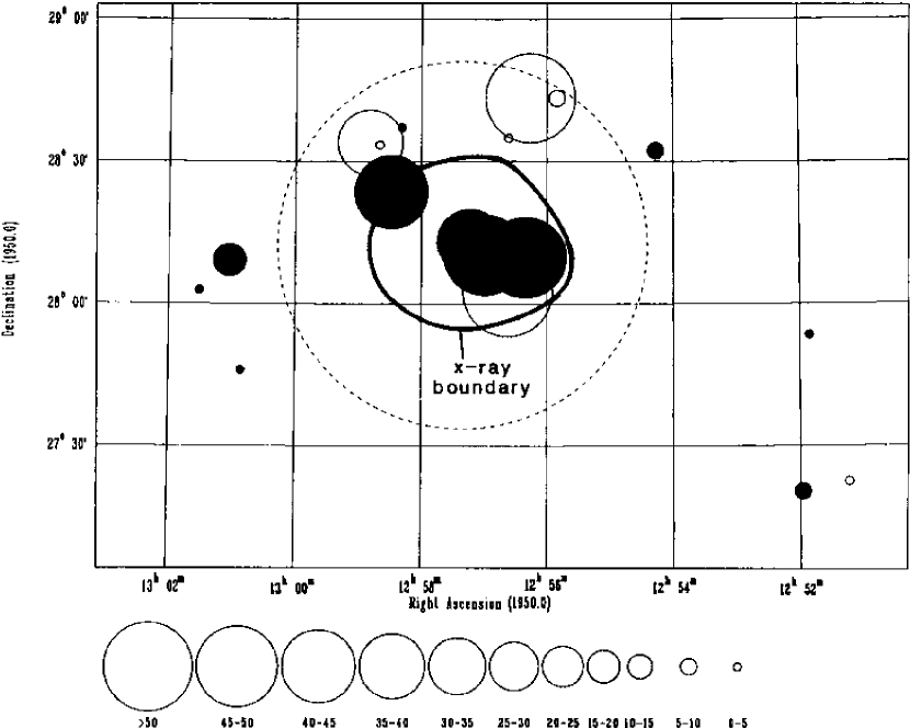
Figure 1: Rotation measures observed in the Coma cluster (reproduced from Kim et al. 1990). The size of the circles indicates the absolute value of RM, the type (filled or empty) the sign of RM. The X-ray boundary (solid curve) and the Abell radius (dashed circle) are superposed to mark the position of the Coma cluster in the plot. The RM pattern can later be compared with our simulated results as shown in Fig. 4.

2 GrapeSPH combined with MHD

We start with the GrapeSPH code developed and kindly provided by Matthias Steinmetz (Steinmetz 1996). The code is specialised to the “Grape” (Gravity Pipe) hardware briefly described below. It simultaneously computes with a multiple time-step scheme the behaviour of two matter components, a dissipation-free dark matter component interacting only through gravity, and a dissipational, gaseous component. The gravitational interaction is evaluated on the Grape board, while the hydrodynamics is calculated by the CPU of the host work-station in the smooth-particle approach (SPH). We supplement the code with the magneto-hydrodynamic equations to follow the evolution of an initial magnetic field caused by the flow of the gaseous matter component.

We briefly describe here the Grape board and SPH as far as necessary for our purposes.

2.1 GRAPE

Gravitational forces are calculated on the special-purpose hardware component Grape 3Af (Ito et al. 1993) which is connected to a Sun-Sparc 10 work-station operating at 50 MHz. Given a collection of particles, their masses and positions, the Grape board computes their mutual distances and the gravitational forces between them, smoothed at small distances according to the Plummer law. A fixed particle (index $a$) at position $\vec{r}_{a}$ with velocity $\vec{v}_{a}$ thus experiences the gravitational acceleration

$$\left(\frac{{\rm d}\vec{v}_{a}}{{\rm d}t}\right)_{\mathrm{grav}} = \sum_{i}\frac{m_{i}}{(|\vec{r}_{a}-\vec{r}_{i}|^{2}+0.25(\epsilon_{a}+\epsilon_{i})^{2})^{1.5}}$$ (2)

$$\times (\vec{r}_{a}-\vec{r}_{i})\;,$$

with the sum running over all other particles $i$ at positions $\vec{r}_{i}$ and with masses $m_{i}$. The softening length $\epsilon$ is adapted to the mass of each particle to prevent floating-point overflows beyond the restricted dynamical range of the Grape hardware. Conveniently, the Grape board also returns a list of neighbouring particles to a given particle, which is helpful later on for the SPH part of the code.

2.2 SPH

Smoothed-particle hydrodynamics (SPH; Lucy 1977; Monaghan 1985) replaces test particles by spheres with variable radii. An ensemble of such extended particles with masses $m_{i}$ at positions $\vec{r}_{i}$ then gives rise to the average mass density at position $\vec{r}$,

$$\langle\rho(\vec{r})\rangle=\sum_{i}\,m_{i}\,W(\vec{r}-\vec{r}_{i},h)\;.$$ (3)

The spatial extent of the particles is specified by the SPH kernel $W(\delta\vec{r},h)$ which depends on the distance $\delta\vec{r}$ from the point under consideration and has a finite width parameterised by $h$. The kernel must be normalised, and approach a Dirac delta distribution for vanishing $h$. A normalised Gaussian fulfils these conditions, but for numerical purposes kernels with compact support are preferred. We use the $B_{2}$-spline kernel (Monaghan 1985). The summation over all particles is then effectively reduced to a summation over neighbouring particles.

Physical quantities $A$ are calculated at the particle positions $\vec{r}_{b}$ and extrapolated to any desired position $\vec{r}$ in an analogous manner,

$$\langle A(\vec{r})\rangle=\sum_{b}\,m_{b}\,\frac{A(\vec{r}_{b})}{\rho(\vec{r}_{b})}\,W(\vec{r}-\vec{r}_{b},h)\;,$$ (4)

where $b$ runs over all particles within a neighbourhood of $\vec{r}$ specified by $h$, and $m_{b}\,\rho^{-1}(\vec{r}_{b})$ represents the volume element occupied by the $b\,$th particle. The crucial step in SPH is to identify the averaged quantity $\langle A(\vec{r})\rangle$ from eq. (4) with the physical quantity $A(\vec{r})$.

According to eq. (4), spatial derivatives of $A(\vec{r})$ can be expressed as sums over $A(\vec{r}_{b})$ times spatial derivatives of the kernel function, which are analytically known from the start. Thus,

$$\nabla A(\vec{r})=\sum_{b}\,m_{b}\,\frac{A(\vec{r}_{b})}{\rho(\vec{r}_{b})}\,\nabla W(\vec{r}-\vec{r}_{b},h)\;.$$ (5)

The hydrodynamic equations are correspondingly simplified. Here we need the derivatives at a particle position $\vec{r}_{a}$. We therefore replace $\vec{r}$ by $\vec{r}_{a}$ and mark the gradient operator with a subscript $a$ to indicate that the gradient is to be taken with respect to $\vec{r}_{a}$. The momentum equation can then be written

$$\left(\frac{{\rm d}\vec{v}_{a}}{{\rm d}t}\right)_{\mathrm{hyd}} = \sum_{b}\,m_{b}\,\left(\frac{P_{b}}{\rho_{b}^{2}}+\frac{P_{a}}{\rho_{a}^{2}}+\Pi_{ab}\right)$$ (6)

$$\times \nabla_{a}W(\vec{r}_{a}-\vec{r}_{b},h)\;,$$

and the equation for the internal energy $u_{a}$ takes the form

$$\frac{{\rm d}u_{a}}{{\rm d}t} = \sum_{b}\,m_{b}\,\left(\frac{P_{b}}{\rho_{b}^{2}}+\frac{1}{2}\,\Pi_{ab}\right)\,(\vec{v}_{a}-\vec{v}_{b})$$ (7)

$$\times \nabla_{a}W(\vec{r}_{a}-\vec{r}_{b},h)\;.$$

These equations need to be supplemented by an equation of state. We assume an ideal gas with an adiabatic index of $\gamma=5/3$, for which the pressure is given by $P_{i}=(\gamma-1)\,u_{i}\rho_{i}$. The tensor $\Pi_{ij}$ describes an artificial viscosity term required to properly capture shocks. We adopt the form proposed by Monaghan & Gingold (1983) and Monaghan (1989) which includes a bulk-viscosity and a von Neumann-Richtmeyer viscosity term, supplemented by a term controlling angular-momentum transport in presence of shear flows at low particle numbers (Balsara 1995, Steinmetz 1996).

The code automatically adapts the spatial kernel $W(\vec{r}_{a}-\vec{r}_{b},h)=0.5[W(\vec{r}_{a}-\vec{r}_{b},h_{a})+W(\vec{r}_{a}-\vec{r}_{b},h_{b})]$ and its width $h_{i}$ for each particle in such a way that the number of neighbouring particles falls between 50 and 80. This results in an adaptive spatial resolution which depends on the mass of the SPH particle and the local mass density at the particle position, because the number of neighbours is determined by the local density and the particle mass.

2.3 MHD

For an ideally conducting plasma, the induction equation can be written as

$$\frac{{\rm d}\vec{B}}{{\rm d}t}=(\vec{B}\cdot\nabla)\vec{v}-\vec{B}(\nabla\cdot\vec{v})+\vec{v}(\nabla\cdot\vec{B})\;.$$ (8)

Theoretically of course, the last term in eq. (8) can be ignored. Numerically however, $\nabla\cdot\vec{B}$ will not exactly vanish, and therefore the question arises whether the actual or the ideal divergence should be inserted when numerically evaluating the induction equation. We performed tests showing that including $\nabla\cdot\vec{B}$ in eq. (8) results in a strong increase of any initial $\nabla\cdot\vec{B}$ as time proceeds. When we set $\nabla\cdot\vec{B}=0$, however, an initially small but non-vanishing divergence rises at most in proportion to $|\vec{B}|$, thus remaining negligibly small.

The field acts back on the plasma with the Lorentz force

$$\vec{F}=-\nabla\left(\frac{\vec{B}^{2}}{8\pi}\right)+\frac{1}{4\pi}(\vec{B}\cdot\nabla)\vec{B}\;.$$ (9)

Formally inserting $\nabla\cdot\vec{B}$ into this expression, the magnetic force can be written as the divergence of a tensor ${\cal M}_{ij}$,

$$F_{j}=\frac{\partial{\cal M}_{ij}}{\partial x_{i}}\;,$$ (10)

with components of ${\cal M}$ given by

$${\cal M}_{ij}=\frac{1}{4\pi}\,\left(\vec{B}_{i}\vec{B}_{j}-\frac{1}{2}\vec{B}^{2}\delta_{ij}\right)\;.$$ (11)

The two formally equivalent expressions (9) and (10) for the magnetic force have different advantages.

Manifestly in conservation form, eq. (10) conserves linear and angular momenta exactly. However, for strong magnetic fields, i.e. fields for which the Alfvén speed is comparable or larger than the sound speed, motion can become unstable (Phillips & Monaghan 1985). In our cosmological cluster simulations, magnetic fields never reach such high values, so we can safely employ eq. (10). We compared cluster simulations performed with both force equations (9) and (10), finding no significant differences in the resulting magnetic field. Nonetheless, we switched to eq. (9) for the tests described below in which strong magnetic fields occur. As expected, results are improved in such cases. This is partially due to the fact that the shock tube problem described in Sect. 4.1 has an unphysical divergence in $\vec{B}$ at the shock.

In the language of SPH, eqs. (8) and (10) read

$$\frac{{\rm d}\vec{B}_{a,j}}{{\rm d}t} = \frac{1}{\rho_{a}}\,\sum_{b}\,m_{b}\,(\vec{B}_{a,j}\vec{v}_{ab}-\vec{B}_{a}\vec{v}_{ab,j})$$ (12)

$$\times \nabla_{a}W(\vec{r}_{a}-\vec{r}_{b},h)\;,$$

and

$$\left(\frac{{\rm d}\vec{v}_{a}}{{\rm d}t}\right)_{\mathrm{mag}} = \sum_{b}\,m_{b}\,\left[\left(\frac{{\cal M}}{\rho^{2}}\right)_{a}+\left(\frac{{\cal M}}{\rho^{2}}\right)_{b}\right]\,$$ (13)

$$\times \nabla_{a}W(\vec{r}_{a}-\vec{r}_{b},h)\;.$$

Here, comma-separated indices $j$ mean the $j\,$th component of any vector. Note that $\nabla_{a}W(\vec{r}_{a}-\vec{r}_{b},h)$ is a vector and therefore leads to a scalar product in eq. (12), and to a matrix product with ${\cal M}$ in eq. (13).

3 Initial conditions

We need two types of initial conditions for our simulations, namely (i) the cosmological parameters and initial density perturbations, and (ii) the properties of the primordial magnetic field. We detail our choices here.

3.1 Cosmology

For the purposes of the present study, we set up cosmological initial conditions in an Einstein-de Sitter universe (${\Omega^{0}_{\rm m}}=1$, ${\Omega^{0}_{\Lambda}}=0$) with a Hubble constant of $H_{0}=50\,{\rm km\,s^{-1}\,Mpc^{-1}}$. We initialise density fluctuations according to a COBE-normalised CDM power spectrum.

The mean matter density in the initial data is determined by the current density parameter ${\Omega^{0}_{\rm m}}$. The Hubble expansion, calibrated by the Hubble constant $H_{0}$, is represented by an isotropic velocity field, which is appropriately added to the initial peculiar velocities of the simulation particles. We use $H_{0}$ in units of $100\,{\rm km\,s^{-1}\,Mpc^{-1}}$ as dimensionless Hubble constant instead of the conventional $h$ to avoid confusion with the width of the SPH kernel. A cosmological constant ${\Omega^{0}_{\Lambda}}$ could be introduced by adding the term

$$\left(\frac{{\rm d}\vec{v}_{a}}{{\rm d}t}\right)_{\mathrm{cos}}={\Omega^{0}_{\Lambda}}\,H_{0}^{2}\,\vec{x}_{a}$$ (14)

to the force equation, according to Friedmann’s equations.

Density fluctuations normalised such as to reproduce the local abundance of galaxy clusters (White, Efstathiou & Frenk 1993) can be mimicked by interpreting simulations at redshift $z>0$ as corresponding to $z=0$. We then have to use $H(z)$ instead of $H_{0}$, and the normalisation is reduced by $(1+z)^{-1}$. $\Omega_{\rm m}(z)$ and $\Omega_{\Lambda}(z)$ do not change with redshift in an Einstein-de Sitter universe.

3.2 Primordial magnetic fields

The origin of the observed cluster magnetic fields is still unclear. As mentioned in the introduction, various models have been proposed which relate the cluster fields with the field generation in the individual galaxies and subsequent wind-like activity which transports and redistributes the magnetic fields in the intra-cluster medium (e.g. Ruzmaikin, Sokolov & Shukurov 1989; Kronberg, Lesch & Hopp 1999). Such scenarios are connected with the observations of metal-enriched material in the cluster, which presume a significant enrichment by galactic winds. However, Goldshmidt & Rephaeli (1994) give strong arguments against intracluster magnetic fields being expelled from cluster galaxies.

Alternatively, it has been proposed that the intergalactic magnetic fields may be due to some primordial origin in the pre-recombination era (Rees 1987) or pre-galactic era (Lesch & Chiba 1995; Wiechen, Birk & Lesch 1998). The first class of models can be disputed on the grounds of principal plasma-physical objections concerning the electric conductivity at the very high temperature stages of the very early universe. The proton-photon and electron-photon collisions produce such a high resistance that primordial magnetic fields are likely not to survive (Lesch & Birk 1998).

The second category (the pre-galactic models) do not reach sufficient field strengths to account for the micro-Gauss fields observed in the intra-cluster medium. Thus we are left with the wind mechanism, which transports magnetic flux into the cluster medium. The initial configuration depends a lot on the time scale on which the magnetic flux is transported into forming cluster structures. If galaxies, especially dwarf galaxies, are formed much earlier than galaxy clusters, they can generate and redistribute magnetic fields very early. This would probably lead to large-scale magnetic fields of about $10^{-9}\,{\rm G}$ on Mpc scales (Kronberg, Lesch & Hopp 1999). If the cluster fields are due to winds from galaxies which later become part of the cluster, the initial field configuration will not be that simple. Taking into account the high velocity dispersion of individual galaxies in clusters and the high electrical conductivity of the plasma, we must expect that the initial cluster field exhibited a very chaotic structure and only the mass flow into and within the cluster can order and amplify it to the observed field strengths.

The simulations presented here start with both set-ups of the primordial magnetic field, namely either a chaotic or a completely homogeneous magnetic field at high redshift. The average magnetic field energy is fixed to the same value in both cases to allow a fair comparison of the results.

The homogeneous magnetic field can be superposed in an arbitrary spatial direction, for which we have chosen the direction of one of the coordinate axes.

To set up the random field, we draw Fourier components of the field strengths, $|\vec{B}_{k}|$, from a power spectrum of the form $P_{\rm B}(k)=A_{0}\,k^{\alpha}$. That is, the $|\vec{B}_{k}|$ are drawn from a Gaussian distribution with mean zero and standard deviation $P_{\rm B}^{1/2}(k)$. To completely specify $\vec{B}$ under the constraint $\nabla\cdot\vec{B}=0$, we choose a random orientation for the wave vector $\vec{k}$ and components of $\vec{B}_{k}$ such as to satisfy $\vec{k}\cdot\vec{B}_{k}=0$. We set the power-spectrum exponent $\alpha=5/3$ corresponding to a Kolmogorov spectrum (Biskamp 1993).

We also vary the strength of the initial magnetic field. We use the average initial field energy density $\langle\vec{B}^{2}\rangle_{\rm ini}/4\pi$ to parameterise initial magnetic field strengths. The magnetic fields are set up at the initial redshift of the simulations, $z=15$.

3.3 Simulation Parameters

Our simulations work with three classes of particles. In a central region, we have $\sim 50,000$ collisionless dark-matter particles with mass $3.2\times 10^{11}\,M_{\odot}$, mixed with an equal number of gas particles whose mass is twenty times smaller. This is the region where the clusters form. At redshift $z=15$ where the simulations are set up, it is is a sphere with comoving diameter $\sim 4.5\,{\rm Mpc}$. The central region is surrounded by $\sim 20,000$ collisionless boundary particles whose mass increases outward to mimic the tidal forces of the neighbouring large scale structure. Including the region filled with boundary particles, the simulation volume is a sphere with (comoving) diameter $\sim 20\,{\rm Mpc}$ at $z=15$.

As mentioned before, the SPH spatial resolution depends on the local mass density. For example, the SPH kernel width $h$ is reduced to $h\approx 100\,{\rm kpc}$ in the centres of clusters at redshift $z=0$. The mean interparticle separation near cluster centres is of order $10\,{\rm kpc}$.

We use a previously constructed sample of eleven different realisations of the initial density field (Bartelmann, Steinmetz & Weiss 1995), to which we add different initial magnetic-field configurations as described before. These density fields were taken out of a large simulation box with COBE-normalised CDM perturbation spectrum (Bardeen et al. 1986) at places where clusters formed in later stages of the evolution. They were re-calculated after adding small-scale power to the initial configurations, taking the tidal fields of the surrounding matter into account.

Generally, we use only the most massive object in the central region of the simulation volume, but for some purposes to be described later, we include up to ten of the next most massive objects found there. The objects are characterised by their virial radii $R_{200}$, which are the radii of spheres within which the average mass density is 200 times the critical density $\rho_{\rm crit}$. The virial mass is then given by $M_{200}=(800\pi/3)\,R_{200}^{3}\rho_{\rm crit}$. All quantities in the code are expressed in physical units. When convenient, we multiply with $H_{0}$ to convert to the conventional units with respect to the dimensionless Hubble constant $H_{0}^{-1}$.

4 Tests of the code

In order to test the code, we follow two strategies. The first consists in re-calculating several test problems, the second in monitoring some quantities in the process of our cosmological simulations, e.g. the $\nabla\cdot\vec{B}$ term.

4.1 Co-planar MHD Riemann problem

A major test of the code is the solution of a co-planar MHD Riemann problem. We compare our results with those obtained with a variety of other methods by Brio & Wu (1988). This problem is a one-dimensional shock tube problem with a two-dimensional magnetic field. For that comparison, we restrict our code to one dimension in space and velocity, and two dimensions in the magnetic field. In addition, we switch off gravitational interactions between particles. We choose 400 SPH particles, which is the same number as Brio & Wu had grid points.

In general, our code clearly and accurately reproduces the results shown by Brio & Wu. In particular, we recover all separate stationary states and waves with correct positions and amplitudes moving into the right directions. However, we also observe particles oscillating around the magnetic shock. The reason for that is that a magnetic discontinuity is set up in such a way that particles, which are driven by the pressure gradient at the shock, are always accelerated towards the discontinuity by the magnetic force. It therefore happens that SPH particles can pass each other or bounce about the discontinuity. This behaviour adds additional high-level noise on top of some of the steady states formed on the low-density side of the shock.

This happens only because the magnetic field is strong enough to produce a magnetic force near the shock which sometimes exceeds the force created by the pressure gradient. We never encountered a comparable situation in our cosmological simulations, where the magnetic force is typically very weak compared to the pressure-gradient or gravitational forces. Such an oscillatory behaviour is therefore not expected to happen in cosmological applications of our code.

4.2 Divergence of $\vec{B}$

As mentioned earlier, our code does not encounter problems with $\nabla\cdot\vec{B}$ as long as we ignore any non-vanishing $\nabla\cdot\vec{B}$ terms in the induction equation (8). The initial magnetic field is specified at SPH particle positions. When extrapolated to grid points, the field acquires a small, but non-vanishing divergence in $\vec{B}$. This initial divergence grows in proportion with $|\vec{B}|$ in the mean, thus remaining negligibly small. Table 1 gives some typical values encountered in our simulations.

Table 1: The growth of the divergence of the magnetic field is illustrated here for one representative cluster simulation with initially homogeneous magnetic field. The 25, 50, and 75 percentiles of the cumulative distribution of $|\nabla\cdot\vec{B}|$ are given for three simulation redshifts $z$. During that time, the magnetic field near the cluster centre rises from $\sim 10^{-9}\,{\rm G}$ to $\sim 10^{-6}\,{\rm G}$, while the 50-percentile (i.e. the median of $|\nabla\cdot\vec{B}|$) increases from $\sim 2.1\times 10^{-35}\,{\rm G\,cm}^{-1}$ to $\sim 1.7\times 10^{-33}\,{\rm G\,cm}^{-1}$.

$z$	$|\nabla\cdot\vec{B}|_{25\%}$	$|\nabla\cdot\vec{B}|_{50\%}$	$|\nabla\cdot\vec{B}|_{75\%}$
	in ${\rm G\,cm}^{-1}$
1.7	$1.6\,10^{-36}$	$2.1\,10^{-35}$	$2.9\,10^{-34}$
0.9	$1.1\,10^{-35}$	$1.4\,10^{-34}$	$2.1\,10^{-33}$
0.0	$1.2\,10^{-34}$	$1.7\,10^{-33}$	$2.3\,10^{-32}$

To relate field strengths and divergences, field strengths need to be divided by a typical length scale, e.g the correlation length of the field. Typically, this is of order $l\sim 50-70\,{\rm kpc}$ in our simulations. Therefore, $B/l\sim 5\times 10^{-30}\,{\rm G\,cm}^{-1}$, approximately three orders of magnitude larger than the median $|\nabla\cdot\vec{B}|$. We also checked the fraction of the cluster volume (defined by a sphere of virial radius) occupied by regions with the largest 10% of $\nabla\cdot\vec{B}$ and found it to be only $\sim 3\%$.

5 Qualitative results

5.1 Importance of shear flows

The magnetic field in our simulated clusters is dynamically unimportant even in the densest regions, i.e. the cluster cores. Since we ignore cooling, this result may change close to cluster centres where cooling can become efficient and cooling flows can form.

The amplification of the magnetic field in a volume element during cluster formation depends on the direction of the magnetic field relative to the motion of the volume element. If the volume element is compressed along the magnetic field line, the strength of the magnetic field is not enhanced at all. If it is compressed perpendicular to the magnetic field lines, the magnetic field strength is enhanced since the number of magnetic field lines per unit volume is increased.

The expected growth of the magnetic seed field due to the formation of a cluster by gravitational collapse can be estimated by the evolution of a randomly magnetised sphere, spherically collapsing due to gravity. Flux conservation leads to an enhancement of the magnetic field proportional to $\rho^{2/3}$. For galaxy clusters, typical overdensities are of order $10^{3}$. This means that starting with magnetic field strengths of order $10^{-9}\,{\rm G}$, spherical collapse can only produce fields of $10^{-7}\,{\rm G}$ strength, an order of magnitude below the $\mu{\rm G}$ fields required to explain observational results.

In our simulations, however, seed fields with $10^{-9}\,{\rm G}$ are indeed amplified to reach $10^{-6}\,{\rm G}$ in final stages of cluster evolution. This is due to shear flows which stretch the magnetic field and amplify it via formation of localised field structures with enhanced strengths. This local amplification is often related to Kelvin-Helmholtz instabilities which form magnetic filaments with much higher field strengths than the surrounding environment. A necessary condition for such an amplification is that the relative velocity on both sides of the boundary layer exceeds the local Alfvén speed which is proportional to the field strength, so that the condition is easy to satisfy for weak initial fields. For galaxy clusters this effect was first discussed by Livio, Regev & Shaviv (1980) and recently simulated in the context of magnetic fields in galaxy haloes by Birk, Wiechen & Otto (1998) who could show that magnetic field strengths are indeed enhanced by a factor of ten by the Kelvin-Helmholtz instability.

Figure 2 illustrates the growth of the magnetic field in a representative cluster. It shows the magnetic field at the position of all SPH particles compared to the mass density at the particle position.

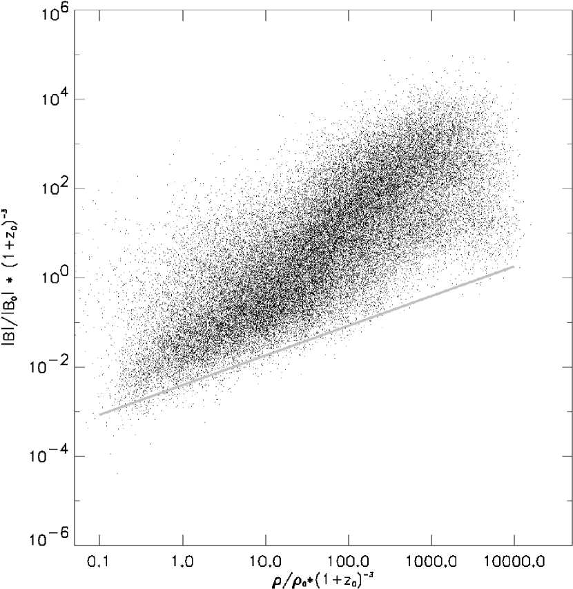
Figure 2: Illustration of the growth of the magnetic field in the simulation volume. For each SPH particle at redshift zero, the absolute magnetic field $|\vec{B}(0)|$ is plotted against the particle density $\rho(0)$. Both $|\vec{B}(0)|$ and $\rho(0)$ are scaled by their values at the initial redshift $z=15$. The line shows the expected $(\rho/\rho_{0})^{2/3}$ behaviour for the magnetic field growth in an isotropic collapse of a randomly magnetised sphere. Evidently, the field growth exceeds the simple collapse prediction for almost all particles.

5.2 Field Structure

As mentioned before, overdensities are a necessary condition for the amplification of magnetic fields, but their presence is not sufficient: Regions with high density but low magnetic field can also occur, depending on the relative directions of compression and magnetic field in a volume element. In addition, the field is also amplified by shear flows. It is therefore not expected that the magnetic field in a cluster acquires an orderly radial profile like, e.g. the density.

Figure 3 shows slices cut through the centres of two of our simulated clusters with different masses. The magnetic field develops a fluctuating pattern of regions with varying field strength, indicated by the gray-scale.

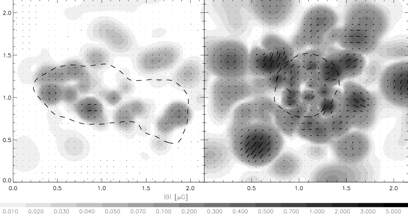
Figure 3: Slices cut through the centres of two simulated clusters are shown here. The gray-scale encodes absolute field strength $|\vec{B}|$ as indicated below the panels. The arrows mark magnetic field vectors in the planes of the slices. Notice that lengths, field strengths, and magnetic field vectors are scaled in the same way in both panels. The contour encloses the region emitting 90% of the slices’ total X-ray luminosity. The cluster shown in the left panel is highly substructured, as can be seen from the elongated X-ray contour. It consists of three main clumps, merging along a common line. Therefore, the X-ray region is more extended than in the more compact cluster shown in the right panel, even though the cluster in the right panel has twice the mass. This more massive cluster has a stronger magnetic field, due to the larger amount of gas compression during its formation.

The fluctuation amplitude clearly increases towards the cluster centres, while the pattern gradually disappears away from the clusters, as is best seen in the left panel. The cluster shown in the right panel exhibits the same behaviour outside the plotted region. The projection of the magnetic field vectors into the slices are also shown as arrows in this illustration. They indicate that the field changes on scales substantially smaller than the cluster scale. The contour encloses the region which emits 90% of the X-ray flux, hence it surrounds the central bodies of the clusters in the panels. The axes are scaled in Mpc.

5.3 Radio and Inverse-Compton Emission

The resolution in our present simulations is not good enough to accurately describe the radio halo of a simulated cluster. Our simulations reliably describe the mean field in clusters only on the resolution scale and above, but we miss any smaller-scale perturbations. For the radio emission, such small-scale fluctuations are important. While small-scale field variations tend to cancel out in the rotation measure because of the line-of-sight integration involved, no such cancellation occurs with the radio emission. Therefore, the mean magnetic field produced by our simulations only provides a lower limit to the radio emission. We will investigate this point in more detail as soon as higher-resolution simulations will become available after an upgrade of our combined Grape-workstation hardware.

So far, we have only performed a consistency check. We assumed that the relativistic electron density is a constant fraction of the thermal electron density, and that the electrons have a power-law spectrum with exponent chosen such as to match the typical exponent of observed radio spectra. The factor between the relativistic and thermal electron densities was chosen such as to reproduce typical radio luminosities; we find it to be of order $10^{-4}$. The question then arises whether such a relativistic electron population would produce unacceptable hard X-ray luminosities through their inverse-Compton scattering of CMB photons. We adapted parameters such as to meet measurements obtained in the Coma cluster (Kim et al. 1990).

We calculated the inverse-Compton emission to find it negligible compared to thermal emission in the soft X-ray bands, which in our example agrees very well with the Coma measurements (Bazzano et al. 1990). As mentioned before, a detailed investigation can only be done with higher-resolution simulations. Nevertheless, this adds to the consistent picture of the clusters in our simulation.

5.4 Faraday Rotation

One way to infer the mean magnetic field strengths in clusters is provided by the Faraday rotation measure. Suppose the magnetic field is randomly oriented and coherent within cells of size $l$. Let $\bar{B}$ be the mean field strength, and $\bar{n}_{\rm e}$ the mean electron density in a cell. The number of cells along the line-of-sight is $\sim l/L$, where $L$ is the extension of the cluster. Then, the expected rms rotation measure is

$$\langle{\rm RM}^{2}\rangle^{1/2}\approx\frac{1}{3}\,812\,\frac{{\rm rad}}{{\rm m}^{2}}\,\left(\frac{l}{L}\right)^{1/2}\,\frac{\bar{n}_{\rm e}}{{\rm cm}^{-3}}\,\frac{\bar{B}}{\mu{\rm G}}\,\frac{l}{{\rm kpc}}\;.$$ (15)

This estimate can be refined by assuming a density profile instead of a constant mean electron density (Taylor & Perley 1993). As long as our simulations properly resolve the coherence scale $l$, the same argument applies to rotation measures obtained from cluster simulations. Hence, observed and synthetic Faraday-rotation measurements provide a sensible way to compare the simulated to observed clusters.

Among other things, Fig. 4 shows the rotation measure for one cluster projected on the sides of its simulation cube. The value of the rotation measure is encoded by the gray-scale, as indicated in the plot. The white dashed line is the projected 90% X-ray contour, thus marking the central body of the cluster in the box. Qualitatively, the simulated RM patterns look very similar to observations as those in Coma shown in Fig. 1. All measurements of a significant RM for Coma fall within the Abell radius (dotted circle). In observations and our simulations alike, they do not much extend beyond the X-ray boundary. In both simulations and observations, we find elongated regions in which the sign of the RM does not change. We also find regions with vanishing rotation measure next to regions with high rotation measure. Close to cluster centres, the rotation measure typically changes sign on much smaller scales than farther out. Coherent RM patches thus become smaller, and they are separated by boundaries of negligible RM. The heights of RM peaks decrease away from the cluster centre. This behaviour is illustrated in the lower right panel of Fig. 6 for the Coma cluster (points).

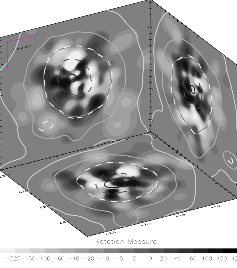
Figure 4: One of the most massive simulated clusters is shown in a three-dimensional box. The Faraday rotation measures produced by the cluster in the three independent spatial directions are projected onto the box sides and encoded by the gray-scale as indicated below the box. The gray solid curves are projected density contours as mentioned in the plot, and the gray dashed curve follows half the central density. The white dashed curve encompasses the region emitting 90% of the projected X-ray luminosity. The cluster is taken from output data at redshift $z=0.5$. The plotted coordinates are physical coordinates, the virial mass is $\approx 20\times 10^{14}\,h^{-1}\,M_{\odot}$, and the virial radius lies outside the box shown.

Patterns in the rotation measure can now statistically be compared across different initial conditions in the simulations, or with comparable statistics of observations.

6 Statistics of Faraday Rotation Measures

6.1 Different Initial Field Set-Ups

To evaluate what the two different kinds of initial magnetic-field set-ups imply for the observations of rotation measures, we compute rotation-measure maps from the cluster simulations and compare them statistically. We use two methods for that. First is the usual Kolmogorov-Smirnov test, which evaluates the probability with which two sets of data can have been drawn from the same parent distribution. Second is an excursion-set approach, in which we compute the fraction ${\cal F}$ of the total cluster surface covered by RM values exceeding a certain threshold. For the cluster surface area, we take the area of the region emitting 90% of the X-ray luminosity.

Figure 5 shows how the RM distributions evolve in clusters in which the initial magnetic field was set up either homogeneously or chaotically. We use the excursion-set approach here, i.e. we plot the fraction ${\cal F}$ of the cluster area that is covered by regions in which the RM exceeds a certain threshold.

Figure 5: This figure shows the fraction ${\cal F}$ of the cluster area which is covered by regions in which the absolute value of the rotation measure exceeds a certain threshold. The cluster area is taken to be the area of the region emitting 90% of the X-ray luminosity. The results are averaged over the three independent spatial directions. Line types distinguish different RM thresholds, as indicated in the figure.

Quite generally, this fractional area for fixed RM threshold increases during the process of cluster formation. There is only little difference between initially homogeneous (heavy lines) and chaotic (thin lines) magnetic fields. At later stages of cluster evolution, the area covered by a minimum rotation measure tends to decrease again. This general behaviour is an effect of sub-structures in clusters: While the clusters form, infalling material creates shocks in the intra-cluster gas, where the magnetic field is amplified by compression, and the motion of accreted sub-lumps through the intra-cluster plasma builds up shear flows which stretch the magnetic field. As the clusters relax, the magnetic field strengths decrease somewhat because of dissipation.

Another way of analysing these patterns is to randomly shoot beams of a certain width through the clusters, determine the average rotation measure in these beams and statistically compare such synthetic Faraday-rotation measurements to observed samples.

We first pick a cluster of $10^{15}\,M_{\odot}$ final virial mass, simulated with both homogeneous and chaotic initial magnetic field configurations, and randomly shoot $10^{4}$ beams through it, along which we compute the Faraday rotation measure. The resulting cumulative RM distributions are shown in Fig. 6, where the solid and dashed curves show results for the homogeneous and chaotic magnetic-field set-up, respectively. Evidently, there is very little difference between these two distributions, indicating that the vastly different initial magnetic-field configurations lead to virtually indistinguishable rotation-measure samples.

Figure 6: Four cumulative rotation-measure distributions are shown in the upper panel. Solid and dashed curves: A cluster model with final virial mass $M_{200}=10^{15}\,M_{\odot}$ was simulated twice, once with a homogeneous (solid curve) and once with a chaotic (dashed curve) initial magnetic field of the same rms strength. At redshift zero, synthetic rotation-measure samples were obtained from both clusters by determining the Faraday rotation along $10^{4}$ beams randomly shot through the clusters. Evidently, the two curves are very similar, indicating that the vastly different magnetic-field set-ups do not lead to any significant difference in the observable RM distributions for a given cluster. For comparison, the dotted curve shows similar results for a cluster with twice the mass, in which the initial magnetic field was homogeneous. The RM variance is substantially increased. This indicates that RM distributions are expected to vary much more strongly with cluster mass than with the initial field configuration. Finally, the dash-dotted curve shows the distribution of the measurements obtained in the Coma cluster. Various corrections detailed in Sect. 7.1 are applied to the latter distribution in the lower panel. Kolmogorov-Smirnov tests show that the Coma measurements are fully compatible with the synthetic RM distributions in the less massive cluster, and incompatible at the 99% level with the simulations in the more massive cluster.

To emphasise this statement, we add to Fig. 6 a short-dashed curve showing the RM distribution obtained from a cluster with twice the final mass, in which the initial magnetic field was set up homogeneously. The curve is much flatter than for the lower-mass cluster, showing that the rms rotation measure is substantially larger in the more massive cluster. Obviously, clusters with different masses produce much more different RM distributions for the same class of magnetic initial conditions than clusters of the same mass do for different classes of initial conditions. Hence, the scatter of results across a sample of clusters with different masses is expected to be much too large to allow to distinguish in principle between the two kinds of magnetic initial conditions.

As an additional difficulty, the number of sources with sufficiently high, sufficiently polarised flux behind a given cluster is fairly limited. Hence, the small number of possible beams measuring RM values in clusters further restricts the power of statistical comparisons between cluster magnetic fields.

6.2 Varying Initial Field Strengths

We now investigate whether this result holds true for a sample of simulated clusters, irrespective of their masses and also their initial magnetic field strengths. For that purpose, we produce a sample of 13 clusters, each of which is simulated twice, once with homogeneous and once with chaotic initial magnetic field. To increase the scatter in mass, we take the clusters at output redshifts between $z=0.78$ and $z=0$. The cluster masses then range within $(8-25)\times 10^{14}\,M_{\odot}$. Initial rms magnetic field strengths are varied between $(1/3-3)\times 10^{-9}\,{\rm G}$.

As before, we then compute RM distributions from $10^{4}$ rays shot randomly through the clusters inside the X-ray boundary, and compare them with a Kolmogorov-Smirnov test. The results show that even 30 RM values per cluster are insufficient to distinguish between the two field set-ups at the 3-$\sigma$ level for all simulated clusters. In particular, in the Coma cluster, which is the best-observed cluster in that respect, there are only ten RM values available within the X-ray boundary.

An important result of these comparisons is that there is no statistically significant difference between the RM patterns exhibited by clusters whose initial magnetic fields were either homogeneous or chaotic. This illustrates that the final field configuration in the cluster is dominated by the cluster collapse rather than the initial field configuration. Approximately on the free-fall time-scale, the initial field is first ordered more or less radially, and when the cluster relaxes later, the field is stirred by shear flows in the intra-cluster gas. Although we started two different sets of simulations with extreme, completely different initial conditions, the resulting fields cannot significantly be distinguished by observations of Faraday rotation. We believe that this scenario is typical for hierarchical models of structure formation, but may be different in e.g. cosmological defect models.

7 Comparison with observed data

7.1 Individual clusters

We can now compare the simulated RM statistics with measurements in individual clusters like Coma or Abell 2319, for which a fair number of measurements is available. The distribution of the RM values as a function of distance to the cluster centre are shown for the Coma cluster as points in Fig. 7. These measurements have the cumulative distribution (dash-dotted curve) shown in Fig. 6. This distribution can now be compared to the RM values obtained from the simulations (other lines in Fig. 7). For a fair comparison, we have to take the radial source distribution on the sky relative to the cluster centre into account. This can easily be achieved by choosing random beam positions under the constraint that their radial distribution match the observed one. In our example, the Kolmogorov-Smirnov likelihood for 30 simulated beams to match the ten measurements in Coma falls between 30% and 50% for the less massive cluster (solid and dashed curves), compared to a few per cent for the more massive one (dotted curve). Note that the less massive cluster has approximately the estimated mass of Coma.

Figure 7: Several radial distributions of simulated and observed rotation measures are shown. RM values observed in Coma are represented by diamonds and the dash-dotted histogram. The solid and long-dashed distributions were obtained from a simulated cluster with mass $\approx 10^{15}\,M_{\odot}$, for homogeneous and chaotic initial magnetic fields, respectively. For the dotted curve, a cluster with approximately twice the mass was used.

Figure 6 indicates that the cumulative RM distribution in Coma is not symmetric about the origin ${\rm RM}=0$, implying $\langle{\rm RM}\rangle\neq 0$ in Coma. It is possible to apply a constant additive correction of $\approx 14\,{\rm rad\,m}^{-2}$ to the Faraday-rotation measurements in Coma to achieve a vanishing mean $\langle{\rm RM}\rangle=0$. This additive correction yields the dash-dotted curve in the lower panel of Fig. 6, labelled as “corrected”.

In addition, we can statistically correct for Faraday rotation intrinsic to the sources using measurements near the Coma cluster, but outside the X-ray boundary. For the simulated RM distributions in the upper panel of Fig. 6, this procedure yields the curves in the lower panel, which can now directly be compared with the dash-dotted line from the corrected Coma measurements. The Kolmogorov-Smirnov likelihood for simulations and observations to agree is then increased by a factor of $\approx 2$ for the particular clusters used. Nonetheless, we only apply those corrections where explicitly mentioned. If we use the estimated masses of Coma or A 2319 to select simulated clusters, we found that for an initial field of $\approx 10^{-9}\,{\rm G}$ at $z=15$ we achieve excellent statistical agreement with the simulated RM distributions.

A more detailed comparison using a sample of simulated clusters with different initial magnetic-field energies leads to the intuitive result that simulated clusters with smaller initial magnetic field need to have larger masses to achieve reasonable agreement with the Coma measurements.

An alternative way to compare the measurements to the simulations is to radially bin the absolute value of RM around the cluster centre. One can then calculate the mean absolute value of RM, the dispersion, or other characteristic quantities of the RM distribution in dependence of radius.

This is illustrated in Fig. 7, where the mean absolute RM value is plotted for the same three clusters as in the previous figures. As mentioned before, due to the intrinsic RM values of the sources, there is a signal left in the observations for $\phi>40^{\prime}$. To match the observations at this angular scale, we apply the additive correction of $7.7\,{\rm rad\,m}^{-2}$, which is the mean absolute RM value for the observed control sample. This value is added to all theoretical curves. The Faraday rotations measured in the Coma cluster (circles) are inserted according to their distance to the cluster centre. Additionally, the radial distribution of the measurements is shown by a histogram (dash-dotted line). Clearly, for the less massive cluster (solid and dashed curves), the agreement with the observations is better than for the more massive one (dotted line), for which the RM reaches too high values near the centre. It is also clearly visible that the difference between the homogeneous and chaotic initial conditions for the magnetic field is insignificant.

7.2 A sample of clusters

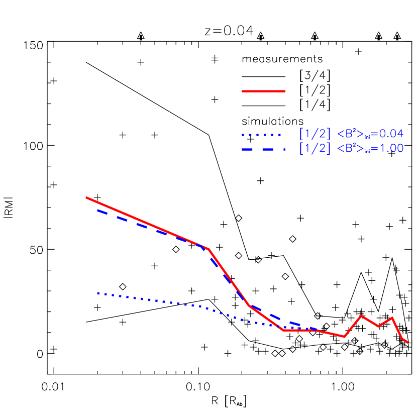
Figure 8: Comparison of simulated results with a sample of measurements in Abell clusters. The absolute values of Faraday rotation measurements (Kim et al. 1991) vs. radius in units of the Abell radius are shown. Obviously, the dispersion increases towards the cluster centre. The solid curves mark the median and the 25- and 75-percentiles of the measurements, and the dashed and dotted curves are the medians obtained from simulated cluster samples starting with high and low magnetic fields, respectively. Specifically, $\langle B^{2}\rangle^{1/2}=10^{-9}\,{\rm G}$ and $0.2\times 10^{-9}\,{\rm G}$ were chosen for the initial rms magnetic field strength. The radial bins are chosen such as to contain 15 data points each. The scatter in the observations is large, but the simulations with the stronger initial magnetic field seem to better match the observations.

Unfortunately, in most clusters the number of radio sources suitable for measurements of Faraday rotation is only one or two. We therefore also compare a sample of simulated clusters with a compilation of RM observations in different clusters. Figure 8 shows the values published by Kim et al. (1991). We take the absolute RM value and plot it against the distance to the nearest Abell cluster in units of the estimated Abell radius (crosses). Measurements in the Coma cluster are marked with diamonds.

The increase of the signal towards the cluster centres is evident. In order not to be dominated by a few outliers, which in some cases even fall outside the plotted region and are marked by the arrows at the top of the plot, we did not calculate mean and variance, but rather the median and the $25$- and $75$-percentiles of the RM distribution (solid curves). We chose distance bins such that each bin contains the same number (15) of Faraday-rotation measurements. We checked that reducing this number to 10 did not change the curves at all.

The median of synthetic radial rotation-measure distributions obtained from our simulations for different initial magnetic field strengths is shown by the dashed and dotted curves. The initial magnetic field strengths for the simulation are indicated by the different line types as indicated in the figure.

In order to correct our synthetic results for source-intrinsic Faraday rotation, we calculate the mean signal in the distance range between one and three Abell radii, and add the resulting $\approx 16\,{\rm rad\,m}^{-2}$ to the simulated curves. Figure 8 shows that an initial field strength of order $\approx 10^{-9}\,{\rm G}$ can reasonably reproduce the observations. We took the simulation at a redshift of $z=0.04$ for this plot, but the results do not change substantially if we take the output at $z=0.5$ to mimic a differently normalised cosmological model.

8 Conclusions

We performed cosmological simulations of galaxy clusters containing a magnetised gas. At redshift $15$, initial magnetic fields of $\approx 10^{-9}\,{\rm G}$ strength were set up, and their subsequent evolution was calculated solving the hydrodynamic and the induction equations assuming perfect conductivity of the intra-cluster plasma. The special-purpose hardware “Grape” was used to calculate the gravitational forces between particles, and the hydrodynamics was computed in the SPH approximation. A previously existing code (GrapeSPH; Steinmetz 1996) was employed and modified to incorporate the induction equation and magnetic forces.

Extensive tests of the code show that it well reproduces test problems and that the divergence of the magnetic field remains negligible during all phases of cluster evolution.

The primary purpose of the simulations was to address two questions. (i) Given primordial magnetic fields of speculative origin and strengths of $\approx 10^{-9}\,{\rm G}$, can simulations reproduce Faraday-rotation observations in galaxy clusters, from which field strengths of order a $\mu{\rm G}$ are inferred? (ii) Is the structure of the primordial fields important, i.e. does it matter for the results whether the fields are ordered on large scales or not? We can summarise our results as follows:

1. Almost everywhere in clusters, the magnetic fields remain dynamically unimportant. Generally, the Alfvén speed is at most $\approx 10$ per cent of the sound speed.

2. While simple spherical collapse models predict final cluster fields of $\approx 10^{-7}\,{\rm G}$, fields of $\mu{\rm G}$ strength are achieved in the simulations. This additional field amplification is due to shear flows in the intra-cluster plasma. Detailed investigations show that particularly strong fields arise in eddies straddling regions of gas flows in different directions.

3. Cumulative statistics of synthetic Faraday-rotation measurements reveal that the cluster simulations reproduce observed RM distributions very well. Generally, more massive clusters require somewhat weaker initial magnetic fields to reproduce observed RM values, but initial field strengths of order $10^{-9}\,{\rm G}$ yield results excellently compatible with observations.

4. Two extreme cases for the structure of the initial fields, namely either completely homogeneous or completely chaotic field structures, lead to final field configurations which are entirely indistinguishable with Faraday-rotation measurements. It is therefore unimportant for interpreting RM observations in clusters how primordial fields are organised as long as they have the right mean strength. The field evolution during cluster formation is thus much more important for the final field structure than any differences in the primordial field structure.

The last item has an important consequence for the epoch when primordial fields need to be in place. Cluster formation is a cosmologically recent process, i.e. it sets in at redshifts below unity. For the field structure in clusters, it is therefore only important that sufficiently strong seed fields be present when cluster formation finally sets in at cosmologically late times. The earlier history of the seed fields is not accessible through cluster observations because information on the primordial field structure is erased during cluster collapse.

We note that our simulations emphasise the role of systematic large-scale flows, i.e. shear flows which are generic constituents of gravitationally unstable multifluid-systems, like collapsing galaxy clusters. Any plasma motion with sufficient velocity gradient will stretch, entangle and disentangle the magnetic field, which is amplified thereby, and since the shear flows in clusters are three-dimensional, the field amplification is a global effect. However, even these intrinsic shear flow patterns have not amplified the field strength to a value where it would be dynamically important; the field is not in equipartition at any stage of the cluster evolution.

An important weakness of our simulations so far is the limited spatial resolution. While we believe that the resolution is sufficient for producing synthetic Faraday-rotation measurements because there magnetic fields are integrated along the line-of-sight so that small-scale fluctuations are averaged out, simulations of the radio emission due to relativistic electrons in the cluster field require higher resolution. We can therefore not use our present simulations to reliably reproduce cluster radio haloes. Nevertheless, we verified using simple assumptions that our cluster simulations meet observational constraints on the hard X-ray emission due to CMB photons which are Compton-upscattered by relativistic electrons. We also note that the field amplification due to shear flows may be somewhat underestimated due to the limited resolution.

The resolution of our simulations will be increased in the near future. They can (and will) then be applied to a number of additional questions related to magnetic fields in clusters, like the structure of radio haloes, the importance of magnetic reconnection for the heat balance in cluster cores, the structure of magnetised cooling flows and so forth.

Finally, we would like to discuss the general lack of diffuse cluster radio haloes (e.g. Burns et al. 1992). We now know that most galaxy clusters contain intracluster fields which are comparable with galactic magnetic field strengths of several $\mu$G (e.g. Kronberg 1994 and references therein), but only a few of them reveal a diffuse radio halo. Why? In view of our simulations this problem is even more severe, since according to our results all galaxy clusters will produce fields of $\mu$G strength, simply by collapse and the accompanying shear flows. Thus, every cluster should shine in the radio.

Here, we would like to present a possible explanation for the missing cluster radio haloes in terms of inefficient particle acceleration in the cluster medium. Our hypothesis is: there is in general no extended radio emission in haloes of galaxy clusters since the number of relativistic electrons is too small, i.e. the particles are not significantly re-accelerated in the cluster.

We can support this hypothesis with two basic arguments:

First, the galaxies in galaxy clusters experience lots of tidal interactions, which excite star formation (SF). Such SF-episodes heat up galaxy haloes and inflate them via galactic winds, which contain cosmic rays and strong magnetic fields (an example par excellence is M82). Thus, these galaxies will slow down the relativistic electrons by considerable synchrotron losses; the energy-loss time $t_{\rm loss}\propto\gamma^{-1}B^{-2}$ decreases with increasing field strength. Therefore, whatever relativistic electron population reaches intergalactic space has already lost a substantial fraction of its energy. Furthermore, the strong shear flows in the intracluster plasma close to the galaxies amplify the halo fields, increase the synchrotron losses and concentrate the high energy particles to the close neighbourhood of the galaxies themselves.

Second, the only possibility to create an extended radio halo would be electron re-acceleration by shock waves or turbulence (Schlickeiser et al. 1987). But, as investigated by Dorfi and Völk (1996), the efficiency of Fermi acceleration of supernova-driven shock waves in hot and tenuous plasmas is drastically reduced. They studied the problem why elliptical galaxies, while containing strong magnetic fields (known from RM-measurements) and enough supernova shocks, do not exhibit significant radio emission. The main reason for the decrease in shock wave acceleration in hot plasmas is the decrease of the Mach number and the decrease of the shock power before the Sedov phase.

Translating their results into the context of galaxy clusters, we would draw the following picture: Relativistic electrons originate in galaxies, they hardly overcome the magnetic barriers of the galactic halo fields. Due to the high sound speed, the shock waves in the cluster medium have only small Mach numbers, and they do not significantly accelerate. The efficiency of MHD turbulence for particle acceleration is also lower in hot, tenuous plasmas since the fluctuations are damped by the hot ions (Holman et al. 1979).

Only external influences like further accretion, especially of cold material, is able to raise the Mach numbers to get significant particle re-acceleration in the clusters (see also Tribble 1993).

References

- [1] Bagchi, J., Pislar, V., Lima Neto, G.B., 1998, MNRAS, 296, L23
- [2] Balsara, D.S., 1995, J. Comput. Phys., 121, 357
- [3] Bardeen, J.M., Bond, J.R., Kaiser, N., Szalay, A.S., 1986, ApJ, 304, 15
- [4] Bartelmann, M., Steinmetz, M., Weiss, A., 1995, A&A, 297, 1
- [5] Bazzano, A., Fusco-Femiano, R., Ubertini, P., Perotti, F., Quadrini, E., Court, A.J., Dean, A.J., Dipper, N.A., Lewis, R., 1990, ApJ, 362, L51-L54
- [6] Biskamp, D., 1993, Nonlinear MHD, Cambridge: University Press
- [7] Birk, G.T., Wiechen, H., Otto, A., 1998, ApJ (submitted)
- [8] Brio, M., Wo, C.C., 1988, J. Comput. Phys., 75, 400
- [9] Burns, J.O., Sulkanen, M.E., Gisler, G.R., Perley, R.A., 1992, ApJ, 388, 21
- [10] De Young, D.S., 1992, ApJ, 386, 464
- [11] Dorfi, E.A., Völk, H.J., 1996, A&A, 307, 715
- [12] Dreher, J.W., Carilli, C.L., Perley, R.A., 1987, ApJ, 316, 611
- [13] Ito, T., Makino, J., Fukushige, T., Ebisuzaki, T., Okumura, S.K., Sugimoto, D., 1993, PASJ, 45, 339
- [14] Feretti, L., Dallacasa, D., Giovannini, G., Tagliani, A., 1995, A&A, 302, 680
- [15] Goldman, I., Rephaeli, Y., 1991, ApJ, 380, 344
- [16] Goldshmidt, O., Rephaeli, Y., 1993, ApJ, 411, 518
- [17] Goldshmidt, O., Rephaeli, Y., 1994, ApJ, 431, 586
- [18] Holman, G.B., Ionson, J.A., Scott, J.S., 1979, ApJ, 228, 576
- [19] Kim, K.T., Kronberg, P.P., Tribble, P.C., 1991, ApJ, 379, 80
- [20] Kim, K.T., Kronberg, P.P., Dewdney, P.E., Landecker, T.L., 1990, ApJ, 355, 29
- [21] Kronberg, P.P., 1994, Rep. Prog. Phys., 57, 325
- [22] Kronberg, P.P., Lesch, H., Hopp, U., 1999, ApJ, 511, 56
- [23] Lesch, H., Chiba, M., 1995, A& A, 297, 305
- [24] Lesch, H., Birk, G.T., 1998, Phys. Plasmas, 5, 2773
- [25] Livio, M., Regev, O., Shaviv, G., 1980, ApJ, 240, L83
- [26] Lucy, L., 1977, AJ, 82, 1013
- [27] Monaghan, J.J., 1985, J. Comput. Phys., 3, 71
- [28] Monaghan, J.J., 1989, J. Comput. Phys., 82, 1
- [29] Monaghan, J.J., Gingold, R.A., 1983, J. Comput. Phys., 52, 374
- [30] Perley, R.A., 1990, IAUS, 140, 463
- [31] Phillips, G.J., Monaghan, J.J., 1985, MNRAS, 216, 883
- [32] Rees, M., 1987, QJRAS, 28, 197
- [33] Rephaeli, Y., 1988, ComAp, 12, 265
- [34] Rephaeli, Y., Gruber, D.E., 1988, ApJ, 333, 133
- [35] Ruzmaikin, A., Sokolov, D., Shukurov, A., 1989, MNRAS, 241, 1
- [36] Schlickeiser, R., Sievers, A., Thiemann, H., 1987, A&A, 182, 21
- [37] Steinmetz, M., 1996, MNRAS, 278, 1005
- [38] Taylor, G.B., Barton, E.J., Ge, J.P., 1994, AJ, 107, 1942
- [39] Taylor, G.B., Perley, R.A., 1993, ApJ, 416, 554
- [40] Tribble, P.C., 1993, MNRAS, 263, 31
- [41] Vallee, J.P., MacLeod, J.M., Broten, N.W., 1986, A&A, 156, 386
- [42] Vallee, J.P., MacLeod, J.M., Broten, N.W., 1987, ApL, 25, 181
- [43] White, S.D.M., Efstathiou, G., Frenk, C.S., 1993, MNRAS, 262, 1023
- [44] Wiechen, H., Birk, G.T., Lesch, H., 1998, A& A 334, 388