Temperature Correlations in a Compact Hyperbolic Universe

Abstract

The effect of a non-trivial topology on the temperature correlations on the cosmic microwave background (CMB) in a small compact hyperbolic universe with volume comparable to the cube of the curvature radius is investigated. Because the bulk of large-angular CMB fluctuations is produced at the late epoch in low $\Omega_{0}$ models, the effect of a long wavelength cut-off due to the periodic structure does not lead to the significant suppression of large-angular power as in compact flat models. The angular power spectra are consistent with the COBE data for $\Omega_{0}\!\geq\!0.1$.

15 August

1 Introduction

Einstein’s equations do not specify the global structure of spacetime. In other words, to a given local metric, a large number of topologically distinct models remain unspecified. In the absence of the unified theory that describes the global structure as well as the local one, one must resort to the observational methods to determine the global topology of the universe.
Assuming that the spatial hypersurface is homogeneous, the observed high degree of isotropy in the cosmic microwave background (CMB) points to the Friedmann-Robertson-Walker (FRW) models as the best candidates of the cosmological models. However, if one would allow the spatial hypersurface being multiply-connected, a variety of locally FRW models which are globally anisotropic and inhomogeneous may be consistent with the current observational data.
Constraints on the topological identification scales using the COBE data have been obtained for some flat models with no cosmological constant (Stevens, Scott & Silk 1993; de Oliveira, Smoot & Starobinsky 1996; Levin, Scannapieco & Silk 1998) and some limited compact hyperbolic (CH) models (Levin, Barrow, Bunn & Silk 1997; Bond, Pogosyan & Souradeep 1998). The large-angular temperature fluctuations discovered by the COBE constrain the possible number of the copies of the fundamental domain inside the last scattering surface to less than $\!\sim$8 for compact flat multiply-connected models.
On the other hand, a large amount of CMB anisotropies on large scales could be produced in the low density universe due to the decay of gravitational potential near the present epoch (Cornish, Spergel & Starkman 1998). Therefore we expect that the constraint on the possible number of copies is less stringent for CH models. However, since the effect of the non-trivial topology becomes more and more significant as the volume of the space decreases, it is very important to investigate the viability of the CH models with small comoving volume.
From a theoretical point of view, the ”smallness” of the spatial hypersurface is an advantage for giving a natural mechanism leading to homogeneity and isotropy. It is well known that geodesic flows on CH spaces are strongly chaotic. Therefore, initial perturbations would be smoothed out due to the mixing effects (Lockhart, Misra & Prigogine 1982; Gurzadyan & Kocharyan 1992; Ellis & Tavakol 1994). In inflationary scenarios, a certain physical process is indispensable that homogenises the initial patch beyond the horizon scale before the onset of inflation for accomplishing the sufficient smoothing of the observable universe (Goldwirth & Piran 1989; Goldwirth 1991). The chaotic mixing in CH spaces may provide a solution to the pre-inflationary initial value problem (Cornish, Spergel & Starkman 1996).
If we live in a small universe which is defined to be a locally homogeneous and isotropic space that is multiply-connected on scales comparable to or smaller than the horizon, the future astronomical satellite missions such as MAP and PLANCK might reveal some specific features in CMB (Cornish, Spergel, & Starkman 1998; Weeks 1998).
So far, a variety of CH manifolds have been constructed by mathematicians. However, the number of the known CH manifolds with small volume is relatively small. In this paper, we investigate CH models whose spatial hypersurface is isometric to the Thurston manifold which is the second smallest in the known CH manifolds with volume 0.98139 times cube of the curvature radius. The smallest one is the Weeks manifold with volume 96 percent of that of the Thurston manifold(see e.g. Fomenko & Kunii 1997). However, the fundamental domain(which tesselates the infinite space) of the Thurston manifold is much simpler than that of the Weeks manifold. For simplicity, we investigate the Thurston models rather than the Weeks models. The fundamental domain of the Thurston manifold is a polygon with 16 faces, which can be constructed by appropriately identifying 8 faces with the remaining 8 faces(see the appendix of Inoue 1999a). It should be noted that the volume of CH manifolds must be larger than 0.16668 times cube of the curvature radius although no concrete examples of manifolds with such small volumes are known (Gabai, Meyerhoff & Thurston 1996).

2 Computation of eigenmodes

So far various kinds of numerical techniques have been proposed to overcome the difficulty of computing the CMB in CH models. For several CH models, CMB fluctuations have been computed using the method of images without carrying out the mode expansion (Bond, Pogosyan, & Souradeep 1998). They obtained the result that the COBE data strongly constrains the CH models so that the comoving volume of the fundamental domain are at least comparable to the comoving volume inside the last scattering surface. Since the method of images requires the sum of exponentially increasing images, it is difficult to obtain the distinct eigenmodes which are necessary to estimate the effect of the power spectrum with discrete peaks. Alternatively, one of the author proposed a numerical approach called the direct boundary element method for computing eigenmodes of the Laplace-Beltrami operator (Inoue 1999a). 14 eigenmodes have been computed for the Thurston manifold. It is numerically found that the expansion coefficients behave as if they are random Gaussian numbers.
In this work, we have numerically computed 36 eigenmodes in the Thurston manifold up to $k\!=\!13$ (the curvature radius is normalized to one) which are approximated by quadrature shape functions which converges to the solutions faster than constant valued shape functions. As we shall see, the contribution of the higher modes to the angular power spectra on large angular scales are relatively small for low-density models. In other words, the effect of the non-trivial topolgy is almost determined by the lower modes. We confirm the previous computed eigenvalues within $|\delta k|\leq 0.01$.
We see from figure 1 that the number of eigenmodes below $k$ is nicely fitted to the Weyl’s asymptotic formula

$$N(k)=\frac{\textrm{Vol}({M})(k^{2}-1)^{3/2}}{6\pi^{2}},~{}~{}~{}k\!>\!>\!1,$$ (1)

where Vol$(M)$ denotes the volume of a manifold $M$. The random Gaussian behavior is again observed for 31 modes $5.404\!\leq\!k\!<\!13$ but five degenerated states have an eigenmode which shows the non-Gaussian behavior due to the global symmetry of the fundamental domain. It is found that the five eigenmodes have $Z2$ symmetry (invariant with respect to the rotation by an angle $\pi$) on the center (where the minimum length of the periodic geodesic which lies on the point is locally maximal) of the fundamental domain. In this case, one would observe an axis around which the fluctuation is rotationally symmetric at the center. Therefore, the correlation between expansion coefficients leads to a non-Gaussian behavior. Nevertheless, it is found that appropriate choices of the linear combination of the degenerated modes recover the generic Gaussian behavior. Furthermore, the symmetry of CH manifolds depends on the observing point. If one randomly choose a point on the manifold, the probability of observing an exact symmetry of the manifold is very small. The result supports the previous investigations of the expansion coefficients which show the Gaussian behavior in classically chaotic systems (Aurich & Steiner 1989; Haake & Zyczkowski 1990) although the global symmetry in the system can hide the generic property (Balazs & Voros 1986).

3 Temperature Fluctuations

Perturbations in CH models can be written in terms of linear combination of eigenmodes on the universal covering space multiplied by the expansion coefficients and the initial fluctuations plus time evolution of the perturbations. The expansion coefficients include the information of the periodicity in the universal covering space. As CH models are locally homogeneous and isotropic, the time evolution of the perturbations coincides with that in open models.

Figure 1: Number function and the Weyl’s asymptotic formula.

The dominant physical effects producing CMB anisotropies (Hu, Sugiyama & Silk 1997) on large angular scales are the ordinary Sachs-Wolfe (OSW) effect (Sachs & Wolfe 1967), which is the gravitational redshift effect in between the last scattering surface and the present epoch, and the integrated Sachs-Wolfe (ISW) effect, which is the gravitational blue-shift effect caused by the decay of gravitational potential at the curvature domination epoch, $1\!+\!z\!\sim\!(1-\Omega_{0})/\Omega_{0}$. For the COBE scales, we can ignore the contribution from the acoustic oscillations. Then the time evolution of the adiabatic growing mode of the Newtonian gravitational potential is analytically given as (see e.g. Kodama & Sasaki 1986; Mukhanov, Feldman & Brandenberger 1992)

$$\Phi_{t}(\eta)=\Phi_{t}(0)\frac{5(\sinh^{2}\eta-3\eta\sinh\eta+4\cosh\eta-4)}{(\cosh\eta-1)^{3}},$$ (2)

where $\eta$ denotes the conformal time. The two-point temperature correlations in a CH cosmological model can be written in terms of the gravitational potential. Assuming that the initial fluctuations obey the Gaussian statistic, and neglecting the tensor-type perturbations, the angular power spectrum $C_{l}$ can be written as

$$(2\,l+1)\,C_{l} = \sum_{m=-l}^{l}\langle~{}|a_{lm}|^{2}\rangle$$ (3)

$$= \sum_{\nu,m}\frac{4\pi^{4}~{}{\cal P}_{\Phi}(\nu)}{\nu(\nu^{2}+1)\textrm{Vol}(M)}~{}|\xi_{\nu lm}|^{2}|F_{\nu l}|^{2},$$

where

$$F_{\nu l}(\eta_{o})\!\!\equiv\!\!\frac{1}{3}\Phi_{t}(\eta_{\ast})X_{\nu l}(\eta_{o}\!-\!\eta_{\ast})\!+\!\!2\!\!\int_{\eta_{\ast}}^{\eta_{o}}\!\!\!\!\!\!d\eta\,\frac{d\Phi_{t}}{d\eta}X_{\nu l}(\eta_{o}\!-\!\eta).$$ (4)

Here, $\nu\!=\!\sqrt{k^{2}-1}$, ${\cal P}_{\Phi}(\nu)$ is the initial power spectrum, and $\eta_{\ast}$ and $\eta_{o}$ are the conformal time of the last scattering and the present conformal time, respectively. $X_{\nu l}$ denotes the radial eigenfunctions in open models and $\xi_{\nu lm}$ denotes the expansion coefficients. From now on we assume that the initial power spectrum is the (extended) Harrison-Zeldovich spectrum $i.e.$, ${\cal P}_{\Phi}(\nu)\!=\!Const.$.
Although the low-lying modes give an appreciable contribution to the large angular power, contributions of higher eigenmodes may not completely be negligible. While the computation of highly-excited eigenmodes is a difficult task, we have so far succeeded to calculate the exact eigenmodes up to $k\!=\!13$ as we mentioned before. However, we are going to assume that $\xi_{\nu lm}$ ’s are also random Gaussian numbers for higher modes. Since the information of the periodicity in the real space is lost by this approximation, we will only employ this approximation to the statistics in the $k$-space which is expected to be not changed because the periodicity is not apparent in the $k$-space. As CH models are globally inhomogeneous, the expected correlation statistics depend on the point of the observer. Therefore, one can interpret that one realization for the expansion coefficients corresponds to a certain point of the observer in the fundamental domain. In order to apply the random Gaussian approximation, one must also estimate the variance of the expansion coefficients. The expansion coefficients are written in terms of eigenmodes $u_{\nu}$ and spherical harmonics $Y_{lm}$ as

$$\xi_{\nu lm}X_{\nu l}(\chi_{o})=\int u_{\nu}(\chi_{o},\theta,\phi)\,Y^{*}_{lm}(\theta,\phi)d\Omega.$$ (5)

It should be noted that (5) is satisfied at arbitrary radius $\chi_{o}$. Let us consider a sphere with large radius $\chi_{o}\!>\!>\!1$ on the Poincar$\acute{\textrm{e}}$ ball which is the image of the upper hyperboloid in the four-dimensional Minkowski space ($y_{0},y_{1},y_{2},y_{3}$) by a stereographic projection onto the unit ball on the ($0,y_{1},y_{2},y_{3}$) plane using a point ($-1,0,0,0$) as the base point. One can expect the random behavior of the mode functions on the sphere as the surface of the sphere which is pulled back by the discrete isometry group fills the fundamental domain ergodically. The (apparent) angular fluctuation scale $\delta\theta$ of $k$-mode is approximated in terms of two parameters $\chi_{o}$ and $k$ as ,

$$\delta\theta^{2}\sim\frac{16\pi^{2}~{}\textrm{Vol}(M)}{k^{2}(\sinh(2(\chi_{o}+r_{ave}))-\sinh(2(\chi_{o}-r_{ave}))-4r_{ave})},$$ (6)

where $r_{ave}$ denotes the averaged radius of the inradius and outradius of the fundamental domain. One can approximate $u_{\nu^{\prime}}(\chi_{o})\sim u_{\nu}(\chi_{o}^{\prime})$ by choosing an appropriate radius $\chi_{o}^{\prime}$ which satisfies $k^{-2}\exp(-2\chi_{o}^{\prime})=k^{\prime-2}\exp(-2\chi_{o})$. Averaging (5) over $l$ and $m$, one obtains

$$\bigl{<}|\xi_{\nu^{\prime}lm}|^{2}\bigr{>}\sim\frac{\exp(-2\chi_{o}^{\prime})}{\exp(-2\chi_{o})}\bigl{<}|\xi_{\nu lm}|^{2}\bigr{>},$$ (7)

which gives $\bigl{<}|\xi_{\nu lm}|^{2}\bigr{>}\sim\nu^{-2}$. We have found that the computed variances of $\xi_{\nu lm}$’s for $2\!\leq l\!\leq 20$, $-l\!\leq m\!\leq l$ are remarkably in good agreement with the analytical estimate.

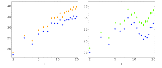
Figure 2: $\delta T_{l}/T\equiv\sqrt{l(l+1)C_{l}/(2\pi)}$ for the Thurston models $\Omega_{0}\!=\!0.2$ (left) and $\Omega_{0}\!=\!0.4$ (right) using expansion coefficients derived from 36 eigenmodes only(stars) and that using these coefficients and random Gaussian numbers for $13\!<\!k\!<\!50$ with 100 realizations (diamonds). Eigenvalues for higher modes are approximated by Weyl’s asymptotic formula.

From figure 2, one can see that the uncertainty in the Gaussian approximation is very small. Remarkably, each realization gives almost the same value so that 100 points for given $l$ are plotted as a tiny speck. The contribution of higher modes becomes significant as $\Omega_{0}$ is increased because the curvature dominant era is shifted to the late time so that the OSW effect becomes dominant over the ISW effect. It is found that contributions of the modes $k\!>\!13$ to $C_{l}$ for $2\!\leq\!l\!\leq\!20$ are approximately $7$ percent and $10$ percent for $\Omega_{0}\!=\!0.2$ and $\Omega_{0}\!=\!0.4$, respectively. Thus contribution of modes $k\!>\!13$ which we employ Gaussian approximation is almost negligible on large angular scales especially in low $\Omega_{0}$ models.

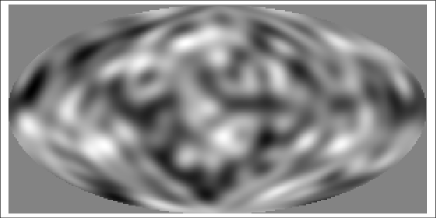
Figure 3: A simulated sky map of the microwave background (convolved with the COBE DMR beam) in the Thurston model $\Omega_{0}=0.2$.

One realization (for the initial fluctuation) of a typical CMB fluctuation as seen by COBE is plotted in figure 3 for $\Omega_{0}\!=\!0.2$. In the simulation, we used only ”exact” 36 eigenmodes. We have chosen a point where the injective radius is maximal as the center (belonging to the ”thick” part of the manifold). One can see that the structure due to the periodical boundary conditions is not apparent. However, approximated number of copies of the fundamental domain inside the last scattering surface is $\sim 500$ for the Thurston model with $\Omega_{0}\!=\!0.2$. Therefore, the effect of the non-trivial topology is expected to be significant.

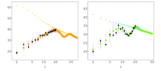
Figure 4: $\delta T_{l}/T\!=\!\sqrt{l(l+1)C_{l}/(2\pi)}$ for the Thurston models at center (diamonds) and ensemble averaged values (boxes) and open models (stars) with $\Omega_{0}=0.2$ (left) and $\Omega_{0}=0.4$ (right). Because of the global inhomogeneity, $\delta T_{l}/T$’s have dependence on the observing points inside the fundamental domain that causes the uncertainty in $\delta T_{l}/T$. Two-sigma ”geometric variance” is shown in vertical lines which has been obtained by $500$ realizations for the expansion coefficients.

The mode cut-off at $k\!=\!5.404$ which corresponds to the largest wavelength inside the fundamental domain causes the suppression of the angular power on large angular scales as in compact flat models. However, the decay of the Newtonian potential in the curvature dominant era makes the difference. Since the bulk of the large angular power comes from the decay of the potential well after the last scattering time, the large angular power does not suffer the significant suppression. We see from figure 4 that the slope of the large angular power is not steep even for the model with $\Omega_{0}\!=\!0.2$ in contrast to the compact flat models without cosmological constant. The two peaks in the power spectrum for the CH model are important in understanding the effect of the non-trivial topology. The angular scale which gives the first peak is equivalent to the angular fluctuation scale of the lowest eigenmode ($k\!=\!5.404$) on the last scattering surface. Substituting the comoving radius of the last scattering surface in unit of the curvature radius $R_{curv}$,

$$R_{LSS}=R_{curv}\cosh^{-1}(2/\Omega_{0}-1)$$ (8)

into (6) gives the angular scales $l\!=\!17$ for $\Omega_{0}\!=\!0.2$ and $l\!=\!7.4$ for $\Omega_{0}\!=\!0.4$. Beyond this scale, the OSW contribution is strongly suppressed as in compact flat models. However, eigenmodes with angular scales below the given scale at the last scattering can have large angular scales after the last scattering. Therefore, in the presence of the ISW effect, the suppression of the power beyond the scale which corresponds to the first peak is very weak in contrast to flat models. The angular scale which gives the second peak corresponds to the scale of the projected lowest eigenmode at the last scattering. Below this scale, the angular power asymptotically converges to that of open models because the effect of the modes with wavelength larger than the cut-off wavelength is negligible. Since we have ignored the effects of subhorizon perturbations at the last scattering such as the so-called ’early’ ISW effect during the matter-radiation equality epoch and the Doppler effect due to the acoustic velocity, the angular power on large to intermediate scales must be slightly boosted. However, these effects are irrelevant to the global effect of the non-trivial topology inasmuch as one considers the typical topological identification scale that is not significantly smaller than the present horizon.

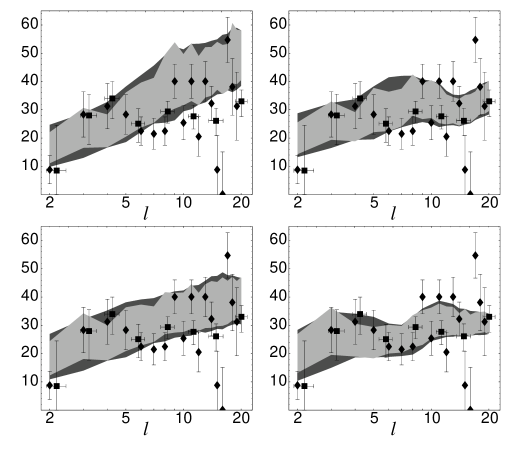
Figure 5: $\delta T_{l}/T\!=\!\sqrt{l(l+1)C_{l}/(2\pi)}$ in $\mu\!K$ for the Thurston model with $\Omega_{0}\!=\!0.1$ (top left) and $\Omega_{0}\!=\!0.4$ (top right) and $\Omega_{0}\!=\!0.2$ (bottom left) and $\Omega_{0}\!=\!0.6$ (bottom right) The light-gray band corresponds to the one-sigma cosmic variance in center and the darkgray band corresponds to the net variance of the one-sigma cosmic and the one-sigma ”geometric” variances. The COBE DMR measurements analysed by Gorski and Tegmark are plotted in diamonds and boxes respectively.

In figure 5, the angular power spectra for low-Omega models are plotted with the COBE data (Gorski et al, 1996) (diamonds). They have been calculated using 36 eigenmodes and the Gaussian approximation taking account of $\sim$10 percent contributions from higher eigenmodes. The slope of the power becomes steep as $\Omega_{0}$ is lowered since the ISW contribution transfers to the large scales.
We have performed a simple $\chi^{2}$ fitting analysis to the COBE DMR band power measurements (Tegmark 1997) (boxes) which are uncorrelated . We have adjusted the normalization of the initial power to minimise the value of $\chi^{2}$. As shown in table 1, the angular power for a model with $\Omega\!=\!0.1$ is still within the acceptable range. The apparent primordial spectral index is approximately $n\!=\!1.6$ for $\Omega\!=\!0.1$.

$\Omega_{0}$	0.1	0.2	0.3	0.4	0.5	0.6
$\chi^{2}$	10.6	6.29	6.42	4.21	4.33	5.20
$Q$	0.15	0.51	0.49	0.76	0.74	0.64

Table 1: $\chi^{2}$ and the probability $Q$ that $\chi^{2}$ should exceed a particular value by chance assuming that $\chi^{2}$ obeys the chi-square distribution with 7 degrees of freedom.

4 CONCLUSIONS

Thus the Thurston models with $\Omega\!\geq\!0.1$ are not constrained by the angular power spectrum from the COBE data, which confirms the preliminary result by one of the author (Inoue 1999b). The peak at $l\!\sim\!4$ in the COBE data may be merely the coincidence due to the large cosmic variance but it is interesting that a model with $\Omega_{0}\!\sim\!0.6$ has the first peak in this scale. Consequently, the Thurston models agree well with the COBE data than any FRW models. The similar conclusion that the constraints $\Omega\!\geq\!0.3$ for an orbifold model with volume $0.7173068R_{curv}^{3}$ have been obtained in (Aurich 1999). Although orbifolds have singular points, the behavior of eigenmodes for orbifolds is expected to be similar to that of manifolds. Therefore, the result for an orbifold model supports our conclusion.

References

- [1]
- [2] Stevens D., Scott D. & Silk J.,1993, Phys. Rev. Lett.,71,20
- [3] de Oliveira-Costa A., Smoot G.F. & Starobinsky A.A.,1996, Astrophys. J., 468,457
- [4] Levin J., Scannapieco E. & Silk J.,1998, Phys. Rev. D,58,103516; preprint (astro-ph/9811226 accepted MNRAS)
- [5] Levin J., Barrow J. D., Bunn E.F. & Silk J.,1997, Phys. Rev. Lett.,79,974
- [6] Bond J.R., Pogosyan D., Souradeep T.,1998, Class. Quant. Grav.,15,2671-2687
- [7] Cornish N.J., Spergel D. & Starkman G.,1998, Phys. Rev. D,57,5982
- [8] Lockhart C.M., Misra B. & Prigogine I.,1982, Phys. Rev. D,25,921
- [9] Gurzadyan V.G. & Kocharyan A.A.,1992, Astron. Astrophys.,260,14
- [10] Ellis G. & Tavakol R.,1994, Class. Quantum. Grav.,11,675
- [11] Goldwirth D.S. Piran T.,1989, Phys. Rev.,D40,3263
- [12] Goldwirth D.S.,1991, Phys. Rev. D,43, 3204
- [13] Cornish N.J., Spergel D., & Starkman G.,1996, Phys. Rev. Lett.,77,215
- [14] Cornish N.J., Spergel D., & Starkman G.,1998, Class. Quant. Grav., 15,2657; 1998, Proc.Nat.Acad.Sci.,95,82
- [15] Weeks J.,1998, Class. Quant. Grav.,15,2599
- [16] Fomenko A.T. & Kunii T.L.,1997, Topological Modeling for Visualization (Springer-Verlag)
- [17] Inoue K.T,1999a, Class. Quant. Grav.,16,3071
- [18] Gabai D, Meyerhoff R. and Thurston N.,1996, MSRI preprint 1996-058 available at http://www.msri.org/
- [19] Aurich R. & Steiner F.,1989, Physica D,39,169
- [20] Haake F. & Zyczkowski K.,1990, Phys. Rev. A,42,1013
- [21] Balazs N.L. & Voros A.,1986, Phys. Rep.,143,No. 3,109
- [22] Hu W., Sugiyama N. & Silk J.,1997, Nature,386,37
- [23] Sachs R.K. & Wolfe A.M.,1967, Astrophys. J.,147,73
- [24] Kodama H. & Sasaki M.,1986, Prog. Theor. Phys. Supp.,78,1
- [25] Mukhanov V.F., Feldman H.A. & Brandenberger R.H.,1992, Phys. Rep.,215,203
- [26] Grski K.M. et al,1996, Astrophys. J.,464,L11
- [27] Tegmark M.,1997, Phys. Rev. D,55,10,5895
- [28] Inoue K.T.,1999b, in Maiani L., Melchiorri F.& Vittorio N., eds., AIP Conference Proceedings 3K Cosmology 1998, (American Institute of Physics) 343
- [29] Aurich R.,1999, Astrophys. J., 524,497