Modeling the Motion and Distribution of Interstellar Dust inside the Heliosphere

Abstract

The interaction of dust grains originating from the local interstellar cloud with the environment inside the heliosphere is investigated. As a consequence of this interaction the spatial distribution of interstellar dust grains changes with time. Since dust grains are charged in the interplanetary plasma and radiation environment, the interaction of small grains with the heliosphere is dominated by their coupling to the solar wind magnetic field. The change of the field polarity with the solar cycle imposes a temporal variation of the spatial distribution and the flux of small (radius smaller than $0.4\;{\rm\mu m}$) interstellar dust grains in the Solar System, whereas the flux of large grains is constant because of their negligible coupling to the solar wind magnetic field. The flux variation observed by in-situ measurements of the Galileo and Ulysses spacecraft are reproduced by simulating the interaction of interstellar grains with charge-to-mass ratios between $0.5\;{\rm C}\;{\rm kg}^{-1}$ and $1.4\;{\rm C}\;{\rm kg}^{-1}$ with the interplanetary environment.

NASA/Johnson Space Center, Houston, Texas, U.S.A.

1 Introduction

Levy and Jokipii [1976] showed that the dominant force on small dust grains in the Solar System is the Lorentz-force caused by the solar wind magnetic field sweeping by the dust grains, which are charged to a positive surface potential, mainly by electron emission due to solar UV photo-effect. It was concluded that due to the coupling to the radially outward flowing solar wind, small interstellar grains do not exist inside the heliosphere which defines the domain of the solar wind. For big grains, Lorentz-force is less important, because they have smaller charge-to-mass ratios, but from the determination of the size range and size distribution of interstellar grains in our galaxy by fitting the wavelength dependence of extinction of starlight on its way through the interstellar medium [e.g. Mathis et al., 1977], it was believed that typical interstellar grains are not larger than $0.5\;{\rm\mu m}$ in diameter. So the conclusion was drawn that there are no big interstellar dust grains and the small ones are swept out of the Solar System by the solar wind magnetic field. Gustafson and Misconi [1979] on the other hand, argued that the electromagnetic interaction enhances the spatial density of small (radii between $0.0005\;{\rm\mu m}$ and $0.12\;{\rm\mu m}$) interstellar grains upstream of the Sun. The detection of interstellar grains in the Solar System by the dust detector on-board Ulysses [Grün et al., 1993] and its confirmation by data from the Galileo dust detector [Baguhl et al., 1995] proved the existence of grains larger than $0.5\;{\rm\mu m}$ and that smaller grains can penetrate into the Solar System, although they are depleted in number [Grün et al., 1994]. It was concluded [Grün et al., 1994; Gustafson and Lederer, 1996; Grogan et al., 1996] that the Lorentz-force on interstellar grains not only repels but also focuses them, depending on the configuration of the solar wind magnetic field, and thus on the phase of the solar cycle. The objective of this work is to quantitatively determine the spatial distribution of interstellar dust grains in the Solar System as a function of the solar cycle. To meet this objective, the motion of interstellar grains in the Solar System is simulated by numerically integrating the equation of motion for a big ($N=10^{6}$ to $10^{7}$) set of interstellar grains. In section 2 the assumptions and approximations used in the model are described. Section 3 presents the resulting three-dimensional and time-dependent spatial distributions of grains in the Solar System. The results are discussed and compared with the in-situ measurements of the Ulysses and Galileo spacecraft in section 4.

2 Model Description

As initial conditions, a homogeneous, mono-directional stream of grains is assumed arriving from an upstream direction of $\lambda_{\rm ecl}=259^{\circ}$ (heliocentric ecliptic longitude) and $\beta_{\rm ecl}=+8^{\circ}$ (heliocentric ecliptic latitude). This direction is equal to the upstream direction of interstellar dust grains in the Solar System as it was determined by analyzing the directional information of the Ulysses in-situ measurements [Baguhl et al., 1995; Frisch et al., 1999]. This direction is also compatible with the upstream direction of interstellar neutral helium atoms, determined by the measurements of the Ulysses/GAS experiment [Witte et al., 1996]. It was shown [Grün et al., 1994], that the impact velocity of interstellar grains measured by Ulysses after Jupiter fly-by was compatible with the velocity of the interstellar helium atoms. Because the impact velocity of an individual grain is determined with an uncertainty of factor $2$ by the in-situ measurement [Grün et al., 1992], the helium velocity of $v_{\infty}=25.3\;{\rm km}\;{\rm s}^{-1}$ was adopted for the model. In the simulation, a “wall” of grains is placed at a heliocentric distance of $100\;{\rm AU}$ every time interval $\Delta t$. The wall covers an area of $30\;{\rm AU}\times 30\;{\rm AU}$ for big and $120\;{\rm AU}\times 200\;{\rm AU}$ for small grains, and is $v_{\infty}\Delta t$ thick. Initially the grains are distributed uniformly inside the wall.

The position $\vec{x}$ and velocity $\dot{\vec{x}}$ of each grain as a function of time is determined by integrating the equation of motion given by:

$$\ddot{\vec{x}}+\left(1-\beta\right)\frac{GM_{\odot}}{\left|\vec{x}\right|^{3}}\vec{x}-\frac{q}{m}\left(\left(\dot{\vec{x}}-\vec{v}_{\rm sw}\right)\times\vec{B}_{\rm P}\right) = 0,$$ (1)

where $\beta$ is the strength of radiation pressure expressed as the ratio of the magnitude of radiation pressure force to the magnitude of gravity, $G$ is the gravitational coupling constant, $M_{\odot}$ the mass of the Sun, $q$ and $m$ the charge and mass of the grain, $\vec{v}_{\rm sw}$ the solar wind velocity, and $\vec{B}_{\rm P}$ the solar wind magnetic field. In the case $q/m\rightarrow 0$, i.e. if the Lorentz-force on the grains is negligible, the spatial distribution of grains can be determined analytically [Landgraf and Müller, 1998] and the solution is rotationally symmetric about the axis parallel to the upstream direction. If the Lorentz-force can not be neglected, the solution to equation (1) has no continuous symmetry and the dust grain trajectories are essentially three-dimensional. Equation (1) contains three basic parameters: the strength of radiation pressure $\beta$, the charge-to-mass ratio $q/m$, and the strength of the radial $B_{r,0}$ and azimuthal $B_{\phi,0}$ components of the solar wind magnetic field. To reduce the number of free parameters in the model, spherical grains with a constant density of $\rho=2.5\;{\rm g}\;{\rm cm}^{-3}$ are assumed. In this case, $\beta$ and $q/m$ can be expressed as a function of grain radius $a$. In the model the calculation of $\beta$ as a function of grain radius by Gustafson [1994] is used (see also table LABEL:tab_cycle below). In this Mie-theory calculation, the optical constants of “astronomical silicates” introduced by Draine and Lee [1984] are assumed. The parameter $\beta$ reaches its maximum for $a=0.18\;{\rm\mu m}$ and is greater than unity for $0.09\;{\rm\mu m}<a<0.4\;{\rm\mu m}$. In this regime, interstellar grains are effectively repelled by the Sun. For $a\rightarrow 0$, $\beta$ reaches a constant value of $\approx 0.1$, and for $a\rightarrow\infty$, $\beta$ depends on $a$ like $a^{-1}$, which is valid in the limit of geometric scattering.

For the charge on a dust grain in interplanetary space it is assumed that the charging process due to photo-emission of electrons induced by solar UV photons partially balanced by the interplanetary plasma environment produces a positive surface potential of $U=+5\;{\rm V}$ on the grain surface [Grün et al., 1994]. The charge of the grain is then given by

$$q = 4\pi\epsilon_{0}Ua,$$

where $\epsilon_{0}$ is the permeability of the vacuum. Thus, $q/m\propto a^{-2}$, which means that electromagnetic interaction with the solar wind magnetic field is only important for small grains.

In the model, Parker’s [1958] model is used, which has been found to be a good large scale approximation of the observed magnetic field in interplanetary space [Mariani and Neubauer, 1990; Burlaga and Ness, 1993; Smith et al., 1995]. The radial, azimuthal, and normal components ($B_{r}$, $B_{\phi}$, $B_{\theta}$) of the Parker-field can be expressed as a function of location in heliographic coordinates ($r_{\rm hg}$, $\lambda_{\rm hg}$, $\beta_{\rm hg}$):

$$B_{r} = \pm B_{r,0}\left(\frac{r_{0}}{r_{\rm hg}}\right)^{2}$$

$$B_{\phi} = \pm B_{\phi,0}\frac{r_{0}}{r_{\rm hg}}\cos\beta_{\rm hg}$$ (2)

$$B_{\theta} = 0,$$

where $B_{r,0}=B_{\phi,0}=3\;{\rm nT}$ are the radial and azimuthal field strength at $r_{0}=1\;{\rm AU}$, respectively [markciteGustafson, 1994]. The Lorentz-force $\vec{F}_{\rm L}$ on a dust grain in interplanetary space caused by the solar wind magnetic field is dominated by the effect of the field sweeping by the grain with the solar wind speed, because the grain velocity is much smaller than the solar wind velocity. Therefore, the Lorentz-force is governed by the term $(q/m)(B_{\phi}v_{\rm sw})$ (see equation (1)). Although it would seem that the Lorentz-force depends on the solar wind speed, this is not the case, because at higher solar wind speeds, the Parker spiral becomes steeper, and consequently the azimuthal component $B_{\phi}$ is reduced [Gustafson and Misconi, 1979], effectively keeping the Lorentz-force constant. The observed sector structure of the polarity of the solar wind magnetic field has been modeled by Alfven [1977] using a “ballerina model”. This model describes a warped current sheet that separates opposite polarities of the magnetic field in interplanetary space. In the ecliptic, opposite polarities are observed in separate sectors, the boundaries of which are given by the intersections of the current sheet with the ecliptic plane. For dust grains in the considered size-range between $a=0.1\;{\rm\mu m}$ and $a=0.7\;{\rm\mu m}$, the instantaneous polarity can be replaced by an average polarity $\overline{p}$ which is a function of the heliographic latitude $\beta_{\rm hg}$. This averaging process is a good approximation for grains for which the Larmor-frequency is orders of magnitude smaller than the solar rotation frequency $\omega_{\odot}$, therefore,

$$a \gg \sqrt{\frac{3\epsilon_{0}UB_{0}}{\rho\omega_{\odot}}}=8\;{\rm nm},$$

where $B_{0}=3\;{\rm nT}$ is the interplanetary magnetic field strength at $1\;{\rm AU}$ and $\omega_{\odot}=2.7\cdot 10^{-6}$ is the solar rotation frequency (rotational period of 27 days). The effect of the sector structure on very small ($6\;{\rm nm}$ to $10\;{\rm nm}$) dust grains which have been ejected by the Jovian system, has been observed by Ulysses [Zook et al., 1996]. The average polarity $\overline{p}$ seen by a dust grain at heliographic latitude $\beta_{\rm hg}$, is given by

$$\overline{p} = \frac{2}{\pi}\arcsin\frac{\tan\beta_{\rm hg}}{\tan\epsilon}$$ (3)

$$B_{r,\phi} \rightarrow \overline{B}_{r,\phi}=\overline{p}\left|B_{r,\phi}\right|,$$

where $\epsilon$ is the tilt angle of the (equivalent) flat current sheet, that rotates with the $22$-year period of the solar cycle [Gustafson, 1994]. From equation (3) it is clear that the average field strength $\overline{B}_{r,\phi}$ is small at low heliographic latitudes, whereas the instantaneous field strength is high at low heliographic latitudes (see equation (2)). This is because a particle at low latitudes experiences a negative polarity nearly as long as a positive polarity. It was shown [Morfill and Grün, 1979] that the stochastic perturbation of the trajectories of small dust grains by the sectored solar wind magnetic field produces an outward directed diffusion of these grains. This is not taken into account by the model, because the sector structure was removed by using an average polarity.

The average polarity $\overline{p}$ defines the sign of the azimuthal component of the average magnetic field and thus the sign of the Lorentz-force, and because the average polarities in the northern and southern hemispheres are always opposite, the Lorentz-force accelerates dust grains away from the solar equatorial plane for $\overline{p}>0$ and towards this plane for $\overline{p}<0$. The sequence of this focusing/defocusing cycle is shown in table 1.

To simulate the motion of interstellar grains in the heliosphere, equation (1) was integrated by using a simple Runge-Kutta integrator of fourth order [Numerical Recipes, 1992]. After the first grains have completely traversed the heliosphere, the spatial distribution of dust grains has been determined at each time step by counting grains inside each cell of an orthogonal, equidistant grid. The resulting spatial distributions of interstellar grains in the heliosphere are discussed in the following sections.

The model described above uses some non-trivial approximations. For the determination of the basic parameters $\beta$ and $q/m$, a spherical grain shape has been assumed. On the other hand, the observation of the polarization of starlight (for summary see Li and Greenberg [1997]) has shown that interstellar dust grains (at least the part of the population that causes the extinction) must have elongated shapes. A deviation from a spherical shape would increase $q/m$ for the same surface potential $U$, because the charge carriers on the grains are separated by larger distances. The $\beta$-value would also increase for non-spherical particles, because it is proportional to the cross-section-to-volume ratio which is minimal for spheres. It can therefore be concluded that a non-spherical particle of the same size as a spherical one has larger values for the basic parameters $q/m$ and $\beta$, or, a non-spherical particle with the same $q/m$ and $\beta$ values used in the simulation is larger than indicated in table 2. Still, $q/m$ and $\beta$ are quantities that depend on material properties of the grains and have not been measured directly. Therefore, they have to be treated as free parameters.

Another assumption made in the model is the constancy of $q$. Due to short-term variations in the solar wind, the surface potential and thus $q$ is expected to fluctuate. These charge fluctuations have the same effect on the grain’s motion as short-term variations of the ambient magnetic field. As shown above, it is a good approximation to use an average strength of the Lorentz-force, with the averaging time-scale being the Larmor-period of the grain. Furthermore it was shown by Zook et al. [1996], who modeled the motion of very small Jupiter stream particles through interplanetary space, that the effect of charge fluctuations on grain dynamics can be neglected for the grain sizes under consideration.

Finally it can be argued that the solar wind magnetic field is not well represented by a Parker spiral during the solar maximum. The physical situation during solar maximum is a highly disordered field with the polarity distribution showing no clear separation of polarities between the northern and southern heliographic hemisphere [Hoeksema, 1985]. As shown above, the motion of grains in the size range of $0.1\;{\rm\mu m}$ depends only on the average polarity $\overline{p}$. In the highly disordered configuration of the solar maximum, regions of positive and negative polarity act on the grains in a stochastic way, independent of the heliographic latitude of the grain’s position. Therefore $\overline{p}=0$ and thus vanishing average Lorentz-force for all heliographic latitudes is a good approximation of the physical situation during the solar maximum, independent of the actual form of the field lines.

3 Spatial Distributions of Interstellar Dust in the Solar System

The spatial distribution of interstellar grains inside the heliosphere shows how the concentration of grains of different sizes is reduced or enhanced by solar gravity, radiation pressure, and the solar wind magnetic field. To display the distributions that result from the model described in section 2, a coordinate-system is chosen such that the $x$-axis is anti-parallel to the initial velocity vector. The $z$-axis is then chosen to be perpendicular to the $x$-axis and to lie in the plane of the initial velocity vector $\vec{v}_{\infty}$ and the solar rotation axis vector $\vec{\omega}_{\odot}$ (see figure 1). The $y$-axis is set to be perpendicular to the $x$- and $z$-axes such that a right-handed coordinate-system is formed.

The angle $\kappa$ between the downstream-direction and the solar rotation axis (as shown in figure 1), has been determined by fitting the directional information of the Ulysses in-situ measurements. The best fit was achieved at $\kappa=98^{\circ}$ [Frisch et al., 1999].

The result of the simulation is shown for four different grain radii: $0.7\;{\rm\mu m}$, $0.5\;{\rm\mu m}$, $0.3\;{\rm\mu m}$, $0.2\;{\rm\mu m}$, and $0.1\;{\rm\mu m}$. For the dynamical parameters $\beta$ and $q/m$ of these grains see table 2.

The spatial distribution of the $0.7\;{\rm\mu m}$ and $0.5\;{\rm\mu m}$ grains is shown in figure 2. Because of the small charge-to-mass ratio of these grains, the coupling to the time-variable solar wind magnetic field is weak, and therefore their spatial distribution is nearly constant and rotationally symmetric about the $x$-axis (downstream direction). The density enhancement downstream of the Sun is produced by gravitational bending of the grain’s trajectories towards the Sun. Due to their smaller $\beta$-value, the downstream concentration increase of the $0.5\;{\rm\mu m}$-grains is less pronounced. The comparison with the result of the analytical calculation [Landgraf and Müller, 1998], which assumes $q/m=0$, shows that electromagnetic interactions can indeed be neglected for these particles. The spatial distribution of grains with radii of $0.3\;{\rm\mu m}$ is already slightly affected by their interaction with the solar wind magnetic field.

For even smaller grains the interaction with the solar wind magnetic field becomes important, as shown in figure 3, in which the time-sequence of the density distribution of interstellar $0.2\;{\rm\mu m}$-grains in the $x$-$y$-plane (approximately in the ecliptic plane) is displayed. As shown in table 1, the solar maximum 1991 was the end of a focusing cycle. The density enhancement in the $x$-$y$-plane is the result of the focusing of grains to this plane. At the maximum of solar activity the average magnetic field is weak, because the current sheet extends to high heliographic latitudes. In this configuration sectors of positive and negative polarity cancel each other efficiently as they pass by the dust grains, creating a weak average Lorentz-force. Therefore, the region of enhanced grain density moves downstream without much perturbation until in 1996 the defocusing effect becomes important. The void region downstream of the Sun is expanded by the defocusing, and the overall density in the $x$-$y$-plane is reduced until the end of the defocusing cycle in 2002. After that the new focusing cycle starts to increase the density in the $x$-$y$-plane until the distribution in 2012 is similar to the one in 1991 when the defocusing cycle started. As a consequence of the large $\beta$-value of $\beta=1.4$, the concentration of $0.2\;{\rm\mu m}$-grains downstream of the Sun is very low. In the $x$-$z$-cut (plane approximately perpendicular to the ecliptic that also contains the stream vector) of the density distribution shown in figure 4 one can see that the density distribution is no longer symmetric about the $x$-axis for $0.2\;{\rm\mu m}$-grains. The first panel in figure 4 also shows that because the upstream direction lies close to but not in the plane of the solar equator, the distribution is asymmetric about the $x$-$y$-plane. At the end of the focusing cycle in 1991 the grains are concentrated along the plane of the solar equator and the density at higher latitudes is reduced. As the defocusing cycle proceeds, the density at higher latitudes increases as more grains are deflected into this region. In 2002, at the end of the defocusing cycle the regions of enhanced density move downstream and the new focusing cycle starts again to concentrate grains around the plane of the solar equator until in 2012 the distribution of 1991 is restored.

The spatial distribution of grains with radii of $0.1\;{\rm\mu m}$ is dominated by the interaction of these grains with the solar wind magnetic field due to their high charge-to-mass ratio of $q/m=5.31\;{\rm C}\;{\rm kg}^{-1}$. At the end of the focusing solar cycle, the grains are concentrated in a sheet about the plane of the solar equator as can be seen in the first panel in figure 6. Because the solar wind magnetic field moves radially outward with the solar wind, the Lorentz-force on the grains is not perfectly perpendicular to the solar equator, but also contains a small outward directed component. This force decelerates small grains and causes a region of enhanced density upstream of the Sun, which is visible as the arc-shaped feature in the first panel of figure 5. As the average field strength is low during the solar maximum, this feature can propagate towards the Sun and the concentration around the plane of the solar equator is split into a northern and southern part by the new defocusing field (1993 to 2001 in figure 6). As can be seen in the panel for 1996 in figure 5, the region of high grain density is diverted before it reaches the solar vicinity. Therefore, the flux of $0.1\;{\rm\mu m}$ grains measured in the solar vicinity (roughly inside Jupiter’s orbit) is expected to be reduced during the full solar cycle due to the interaction with the solar wind magnetic field. This deficiency of small grains has been observed in the in-situ data [Grün et al., 1994; Landgraf et al., 1999]. After a new focusing cycle starts in 2002, grains are again concentrated around the solar equator as can be seen in the panels from 2006 to 2012 in figure 6 until the configuration of 1991 is restored.

The simulation shows that the flux of small interstellar grains in the solar vicinity depends on the phase of the solar cycle. Since in the interstellar medium, small grains ($a<0.2\;{\rm\mu m}$) dominate the dust population by number as indicated by extinction measurements [Mathis et al., 1977; Kim et al., 1994], the total flux of interstellar grains in the Solar System should be dominated by smallest grains that are not filtered by the solar wind magnetic field. Therefore, the total flux of interstellar dust depends on the phase of the solar cycle. In the next section the flux of interstellar grains measured in-situ with the Galileo and Ulysses dust detectors is compared with the temporal variation predicted by the model.

4 Comparison with In-Situ Measurements

The magnitude $f_{\rm isd}(t_{1},t_{2})$ of flux of interstellar dust measured by the dust detectors on-board Ulysses and Galileo in the time-interval $[t_{1},t_{2}]$ is determined by $f_{\rm isd}=N_{\rm isd}(t_{1},t_{2})/I(t_{1},t_{2})$, where $N_{\rm isd}(t_{1},t_{2})$ is the number of interstellar grains detected in the given time-interval and $I(t_{1},t_{2})$ is the average sensitive detector-area, accumulated between $t_{1}$ and $t_{2}$. $I(t_{1},t_{2})$ is given by:

$$I(t_{1},t_{2}) = \int_{t_{1}}^{t_{2}}dt\int_{0}^{2\pi}\frac{d\phi_{\rm rot}}{2\pi}A(t,\phi_{\rm rot})\frac{v_{\rm rel}(t)}{v_{\infty}},$$

where $\phi_{\rm rot}$ is the spacecraft rotation angle (Ulysses and Galileo are spin-stabilized spacecraft, and therefore the sensitive area for a dust stream from one direction has to be averaged over the rotation angle), $A$ is the sensitive detector-area of the dust detector which is a function of time and rotation angle, $v_{\infty}$ is the dust velocity at large distances from the Sun, and $v_{\rm rel}$ is the relative velocity of the spacecraft and the dust as a function of time. By introducing the factor $v_{\rm rel}/v_{\infty}$, the effect of the flux measured in the spacecraft frame being enhanced if the spacecraft moves upwind and reduced during downwind motion is taken into account. Therefore, $f_{\rm isd}$ is the flux in the inertial frame at the location of the spacecraft at time $t$.

In the following $f_{\rm isd}(t)$ predicted by the model is compared with the flux measured with the Ulysses and Galileo spacecraft. For the comparison it is assumed, that the population of interstellar dust grains is dominated by grains out of a narrow size-interval which can be represented by one of the simulated grain-sizes (and thus dynamical parameters $\beta$ and $q/m$). In figure 7 the model prediction for the flux of interstellar grains at the location of the Ulysses and Galileo spacecraft is shown as a function of time.

For the Galileo measurements the simulation predicts a constant flux of interstellar grains on the detector for all but the smallest grain sizes. This is because of the short period of time covered by the Galileo data. Interstellar grains could be identified clearly in the Galileo data only after it left the inner Solar System in mid-1993 and before it reached the Jovian system at the end of 1995. This time interval is short compared to the duration of the solar cycle, therefore the change of the solar cycle did not affect the flux of $0.2\;{\rm\mu m}$- and $0.3\;{\rm\mu m}$-grains. The predicted increase in the flux of $0.1\;{\rm\mu m}$-grains is due to to Galileo’s upstream directed motion towards the region of enhanced spatial density as can be seen in the first three panels of figure 5.

The prediction for the long-term measurements of Ulysses from February 1992 (Jupiter flyby) to end of 1997 (latest data) shows that for $0.1\;{\rm\mu m}$-, $0.2\;{\rm\mu m}$, and $0.3\;{\rm\mu m}$-grains the effects of the solar cycle should modulate the measured flux. In the Ulysses data, the flux of $0.1\;{\rm\mu m}$-grains is predicted to be strongly reduced. After 1996 the simulation predicts a decrease in the flux of the $0.2\;{\rm\mu m}$- and $0.3\;{\rm\mu m}$-grains. This is due to the defocusing effect of the solar wind magnetic field on the trajectories of these grains. The flux of larger grains is nearly constant and close to its value at large distances, because they couple weakly to the solar wind magnetic field.

Figures 8 and 9 show the comparison of the temporal variation of the flux predicted by the simulation with the Galileo and Ulysses in-situ measurements, respectively. Since the spatial density of grains represented by one of the simulated grain sizes at large heliocentric distances is not known, the normalization of the spatial distribution is a free parameter that can be scaled by an overall factor such that the square of the difference of prediction and measurement is minimized. If grains with dynamical parameters similar to the simulated $0.1\;{\rm\mu m}$-, $0.2\;{\rm\mu m}$-, or $0.3\;{\rm\mu m}$-grains dominate the interstellar dust population measured by Galileo and Ulysses, the predicted temporal variation of the flux of the corresponding grain size should match the measurements.

Galileo has measured an increasing flux of interstellar grains on its way to Jupiter. According to the simulation this is best explained with grains that interact strongly with the solar wind magnetic field and are thus deficient in the inner Solar System. Because Galileo was moving upwind to larger heliocentric distances, it detected an increasing flux. The same deficiency of grains in the inner Solar System can be created by the effect radiation pressure, but to explain an increase of flux outside $4\;{\rm AU}$ observed by Galileo, the grains must have very high $\beta$ values of $2.5$ and larger, which is not supported by the Mie-calculations. Compared to the duration of the solar cycle, Galileo spent a short time in the interplanetary space of the outer Solar System. Therefore, the comparison of the Galileo measurements with the results of the simulation is rather ambiguous and does not give any information about the effect of the changing solar cycle on the distribution of interstellar dust grains in the Solar System.

Since the Ulysses measurements cover nearly $6$ years, the effect of the changing solar cycle can be observed in the Ulysses data. The measured flux stayed constant after Ulysses left the ecliptic plane in February 1992 until mid-1996. After that the flux of interstellar grains decreased until it reached its minimal value of $(4\pm 1)\cdot 10^{-5}\;{\rm m}^{-2}\;{\rm s}^{-1}$ at the end of 1997. For $0.1\;{\rm\mu m}$ grains the simulation does not predict a constant flux at the Ulysses location between $1992$ and $1996$. Furthermore, the flux of the simulated $0.1\;{\rm\mu m}$-grains decreases by an order of magnitude within one year after mid-1996. This is also not observed. Therefore, the in-situ measurements as well as the simulation indicates that grains with charge-to-mass ratios of $5\;{\rm C}\;{\rm kg}^{-1}$ or larger do not contribute significantly to the flux of interstellar grains in the Solar System within Jupiter’s orbit. For $0.2\;{\rm\mu m}$- and $0.3\;{\rm\mu m}$-grains (charge-to-mass ratios between $0.5\;{\rm C}\;{\rm kg}^{-1}$ and $1.4\;{\rm C}\;{\rm kg}^{-1}$) the simulation predicts a flux variation that is in good agreement with the observation, though long-term measurements are necessary to confirm the agreement. Interstellar grains with lower charge-to-mass ratios do not show a decrease in flux (see right panel of figure 7). This explains why bigger grains dominate the mass distribution of interstellar grains measured by Ulysses after mid-1996 compared to the mass distribution measured between 1992 and mid-1996 [Landgraf et al., 1999].

5 Conclusion

The model described in section 2 explains the observed time variability of the flux and grain mass distribution of interstellar dust in the Solar System as due to electromagnetic interaction of the grains with the changing solar wind magnetic field. It also shows that very small grains with large charge-to-mass ratios are repelled from the Sun by the average electromagnetic effects. Since the grain size distribution in the LIC is believed to be very steep, the most abundant interstellar grains have charge-to-mass ratios just small enough (or, equivalently, sizes large enough) for their inertia to overcome the electromagnetic repulsion. In this marginal case the electromagnetic perturbation is still strong and defines the spatial distribution of the grains. The knowledge of the spatial distribution of interstellar dust grains can be used to predict in-situ measurements by spacecraft (e.g. Cassini and Stardust) [Landgraf and Müller, 1998] depending on their location in the Solar System.

The simulation has furthermore shown that the spatial distribution of small interstellar dust grains deviates strongly from the distribution of bound, interplanetary grains. This asymmetry as well as the time variability of the spatial distribution can be used to observe the infrared emission of interstellar dust in the Solar System by telescopic means and distinguish it from the radiation emitted by interplanetary grains. Because of the low average spatial density (about $10^{-15}\;{\rm cm}^{-3}$ to $10^{-14}\;{\rm cm}^{-3}$) of interstellar grains, an instrument of very high sensitivity is needed for such an observation.

Further long-term in-situ measurements are needed to confirm the time variation of the interstellar dust flux discovered in the Ulysses data. The simulation has shown that even small interstellar dust grains reach heliocentric distances of $1\;{\rm AU}$. Therefore, an Earth orbiting satellite can be used to measure or even collect dust grains from outside the Solar System.

Acknowledgments. This work was performed while ML held a National Research Council-NASA/JSC Research Associateship and is based on ML’s PhD thesis “Modellierung der Dynamik und Interpretation der In-Situ-Messung interstellaren Staubs in der lokalen Umgebung des Sonnensystems”, Ruprecht–Karls–Universität Heidelberg, 1998.

References

H. Alfven. Electric Currents in Cosmic Plasmas. Reviews of Geophysics and Space Physics, 15:271–284, 1977.

M. Baguhl, E. Grün, D. P. Hamilton, G. Linkert, R. Riemann, and P. Staubach. The Flux of Interstellar Dust Observed by Ulysses and Galileo. Space Science Reviews, 72:471–476, 1995.

M. Baguhl, D.P. Hamilton, E. Grün, S.F. Dermott, H. Fechting, M.S. Hanner, J. Kissel, B.-A. Lindblad, D. Linkert, G. Linkert, I. Mann, J.A.M. McDonnell, G.E. Morfill, C. Polanskey, R. Riemann, G. Schwehm, P. Staubach, and H.A. Zook. Dust measurements at high ecliptic latitudes. Science, 268:1016–1019, 1995.

L. F. Burlaga and N. F. Ness. Radial and Latitudinal Variations of the Magnetic Field Strength in the Outer Heliosphere. Journal of Geophysical Research, 98(A3):3539–3549, 1993.

B.T. Draine and H.M. Lee. Optical propoerties of interstellar graphite and silicate grains. Astrophysical Journal, 285:89–108, 1984.

P. C. Frisch, J. Dorschner, J. Geiß, J. M. Greenberg, E. Grün, M. Landgraf, P. Hoppe, A. P. Jones, W. Krätschmer, T. J. Linde, G. E. Morfill, W. Reach, J. Slavin, J. Svestka, A. Witt, and G. P. Zank. Dust in the local interstellar wind. submitted to ApJ, 1999.

K. Grogan, S.F. Dermott, and B.Å.S. Gustafson. An estimation of the interstellar contribution to the zodiacal thermal emission. Astrophysical Journal, 472:812–817, 1996.

E. Grün, H. Fechtig, M.S. Hanner, J. Kissel, B.-A. Lindblad, D. Linkert, D. Maas, G.E. Morfill, and H.A. Zook. The galileo dust detector. Space Science Reviews, 60:317–340, 1992.

E. Grün, B.Å.S. Gustafson, I. Mann, M. Baguhl, G.E. Morfill, P.Staubach, A.Taylor, and H.A.Zook. Interstellar dust in the heliosphere. Astronomy and Astrophysics, 286:915–924, 1994.

E. Grün, H.A. Zook, M. Baguhl, A. Balogh, S.J. Bame, H. Fechtig, R.Forsyth, M.S. Hanner, M. Horanyi, J. Kissel, B.-A. Lindblad, D. Linkert, G. Linkert, I. Mann, J.A.M. McDonnell, G.E. Morfill, J.L. Phillips, C. Polanskey, G. Schwehm, N. Siddique, P. Staubach, J. Svestka, and A. Taylor. Discovery of jovian dust streams and interstellar grains by the ulysses spacecraft. Nature, 362:428–430, 1993.

B.Å.S. Gustafson. Physics of zodiacal dust. Annual Review of Earth and Planetary Science, 22:553–95, 1994.

B.Å.S. Gustafson and S.M. Lederer. Interstellar grain flow through the solar wind cavity around 1992. In B.Å.S. Gustafson and M.S. Hanner, editors, Physics, Chemistry and Dynamics of Interplanetary Dust, volume 104 of Astronomical Society of the Pacific Conference Series, pages 35–39, 1996.

B.Å.S. Gustafson and N.Y. Misconi. Streaming of Interstellar Grains in the Solar System. Nature, 282:276, 1979.

J.T. Hoeksema. The relationship of the large-scale solar field to the interplanetary magnetic field: what will Ulysses find? In R.G. Marsden, editor, The Sun and the Heliosphere in Three Dimensions, pages 241–254. Astrophysics and Space Science Library, 1985.

S.-H. Kim., P.G. Martin, and P.D. Hendry. The size distribution of interstellar dust particles as determined from extinction. Astrophysical Journal, 422:164–175, 1994.

M. Landgraf, W. J. Baggaley, and E. Grün. Measurements of the Mass Distribution of Interstellar Dust Grains in the Solar System. Journal of Geophysical Research, this issue, 1999.

M. Landgraf and M. Müller. Prediction of the In-Situ Dust Measurements of the Stardst Mission to Comet 81P/Wild 2. Planetary and Space Science, in press, 1999.

E.H. Levy and J.R. Jokipii. Penetration of interstellar dust into the solar system. Nature, 264:423–424, 1976.

A. Li and J.M. Greenberg. A unified model of interstellar dust. Astronomy and Astrophysics, 323:566–584, 1997.

F. Mariani and F. M. Neubauer. The Interplanetary Magnetic Field. In R. Schwenn and E. Marsch, editors, Physics of the Inner Heliosphere I, pages 183–206, Springer-Verlag, Heidelberg, 1990.

J.S. Mathis, W. Rumpl, and K.H. Nordsieck. The size distribution of interstellar grains. Astrophysical Journal, 280:425, 1977.

G. E. Morfill and E. Grün. The motion of charged dust particles in interplanetary space – II. interstellar grains. Planetary and Space Science, 27:1283–1292, 1979.

E.N. Parker. Dynamics of interplanetary gas and magnetic fields. Astrophysical Journal, 128:664–676, 1958.

E. J. Smith, A. Balogh, R. P. Lepping, E. Neugebauer, J. Phillips, and T. Tsurutani. Ulysses Observations of Latitude Gradients in the Heliosperic Magnetic Field. Advances in Space Research, 16:165+, 1995.

Numerical Recipes in C: The Art of Scienfitic Computing ISBN 0-521-43108-5, Cambridge University Press, 1992.

M. Witte, M. Banaszkiewicz, and H. Rosenbauer. Recent results on the parameters of interstellar helium from the ulysses/gas experiment. In R. von Steiger, R. Lallement, and M.A. Lee, editors, The Heliosphere in the Local Interstellar Medium, volume 78 of Space Science Reviews, pages 289–296. Kluwer Academic Publishers, October 1996.

H.A. Zook, M. Baguhl E. Grün, D.P. Hamilton, G. Linkert, J.-C. Liou, R. Forsyth, and J.L. Phillips. Solar wind magnetic field bending of jovian dust trajectories. Science, 274:1501–1503, November 1996.

    M. Landgraf, NASA/Johnson Space Center, Mailcode: SN2, 2101 NASA Road 1, Houston, TX 77058, U.S.A. (e-mail: Markus.K.Landgraf1@jsc.nasa.gov)

Figure 1.: Coordinate-system in which the spatial distribution of interstellar dust in the heliosphere are displayed. The $x$-$y$-plane is close ($<10^{\circ}$ off) to the cliptic. A tilt angle $\kappa$ of $90^{\circ}$ between the downstream-direction and the solar rotation axis is compatible with the determination of the stream-direction, but the best fit to the in-situ data is achieved at $\kappa=98^{\circ}$ [Frisch et al., 1999].

Figure 2.: The spatial distribution of $0.7\;{\rm\mu m}$- (upper two panels) and $0.5\;{\rm\mu m}$- (lower two panels) grains in a $20\;{\rm AU}\times 20\;{\rm AU}$ area in the $x$-$y$-plane. The linear color scale represents the spatial grain density in units of the density at infinity. The two panels on the left have been calculated using the numerical simulation of particle trajectories and the two panels on the right show the result of a analytical calculation for $q/m=0$ but the same $\beta$-values (see table 2). The numerical simulation is in good agreement with the results from the analytical calculation, the deviations result from the limited number of particles and the limited spatial resolution of the simulation. As expected, gravitational focusing is weaker for $0.5\;{\rm\mu m}$-grains due to their higher $\beta$-value.

Figure 3.: Distribution of simulated interstellar $0.2\;{\rm\mu m}$ grains in the $x$-$y$-plane during the solar cycle between 1991 and 2012. The time sequence starts at the upper left panel and ends at the lower right. Time steps are about 2.5 years. Plots are $80\;{\rm AU}\times 80\;{\rm AU}$

.

Figure 4.: Distribution of simulated interstellar $0.2\;{\rm\mu m}$ grains in the $x$-$z$-plane during the solar cycle between 1991 and 2012. The time sequence starts at the upper left panel and ends at the lower right. Time steps are about 2.5 years. Plots are $80\;{\rm AU}\times 80\;{\rm AU}$.

Figure 5.: Distribution of simulated interstellar $0.1\;{\rm\mu m}$ grains in the $x$-$y$-plane during the solar cycle between 1991 and 2012. The time sequence starts at the upper left panel and ends at the lower right. Time steps are about 2.5 years. Plots are $80\;{\rm AU}\times 80\;{\rm AU}$.

Figure 6.: Distribution of simulated interstellar $0.1\;{\rm\mu m}$ grains in the $x$-$z$-plane during the solar cycle between 1991 and 2012. The time sequence starts at the upper left panel and ends at the lower right. Time steps are about 2.5 years. Plots are $80\;{\rm AU}\times 80\;{\rm AU}$.

Figure 7.: The flux of interstellar dust in the inertial frame at the location of Galileo (left panel) and Ulysses (right panel) as a function of time as predicted by the simulation. The magnitude of the flux is normalized to its value at large distances from the Sun. The radius $a$ of the simulated grains increases from the top to the bottom. Major mission events are indicated by dotted vertical lines. In both cases, the flux of small grains varies stronger than the flux of big grains due to their coupling to the solar wind magnetic field. The flux of $0.1\;{\rm\mu m}$-grains strongly reduced at Ulysses locations.

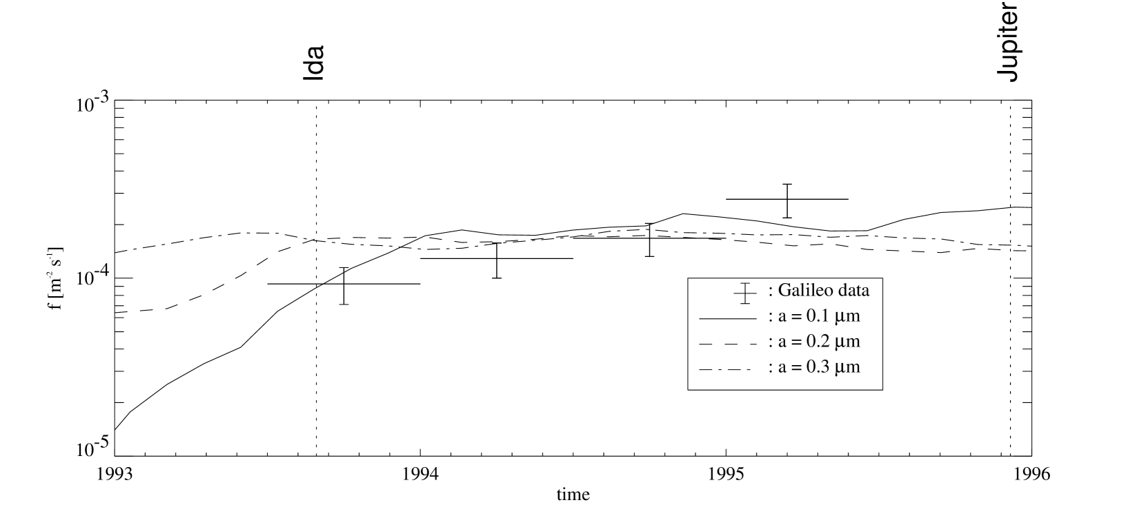
Figure 8.: Comparison of the temporal variation of the flux in the inertial frame at Galileo’s location predicted by the simulation (solid line for $0.1\;{\rm\mu m}$-grans, dashed line for $0.2\;{\rm\mu m}$-grans, and dash-dotted linefor $0.3\;{\rm\mu m}$-grans) with Galileo measurements (crosses). Due to the short time interval covered by the measurements, no significant changes of the flux due to the solar cycle are expected.

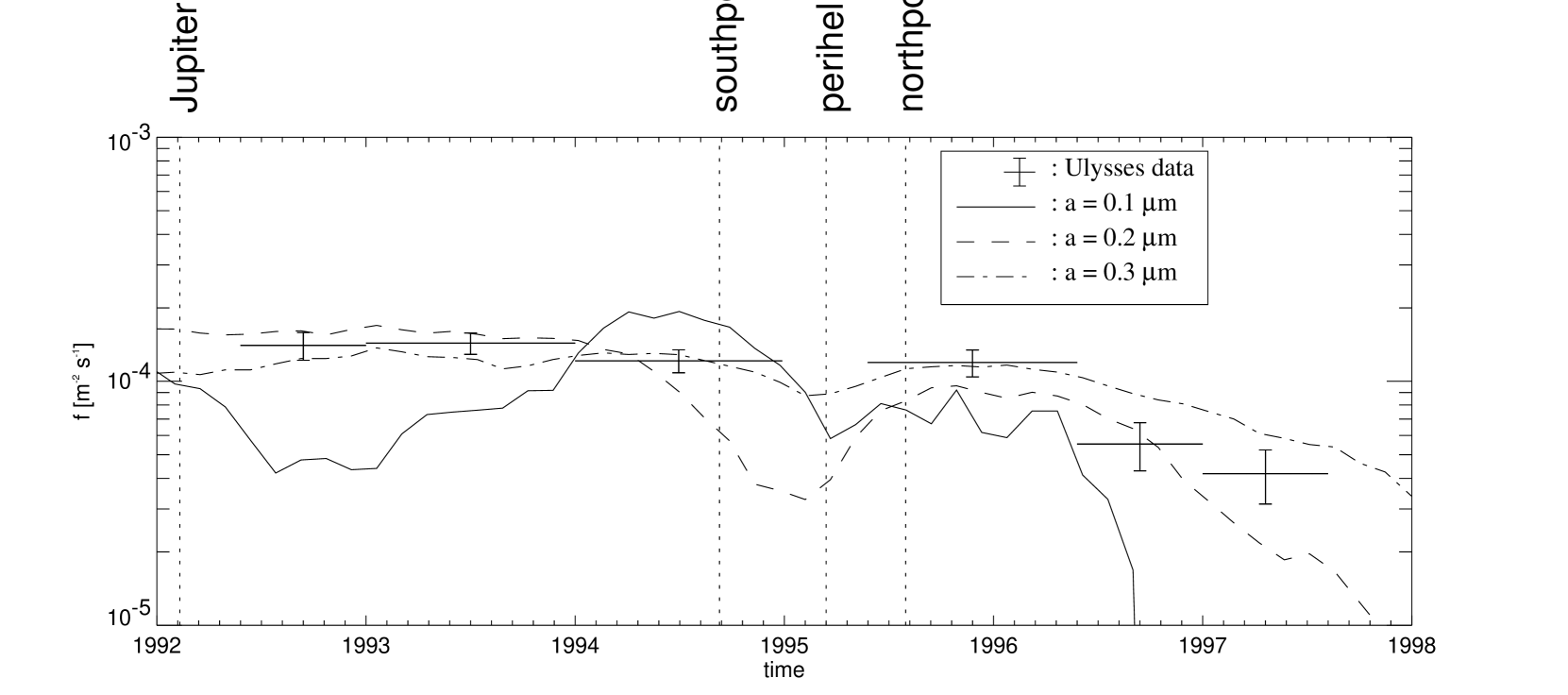
Figure 9.: Comparison of the temporal variation of the flux in the inertial frame at Ulysses’ location predicted by the simulation (solid line for $0.1\;{\rm\mu m}$-grans, dashed line for $0.2\;{\rm\mu m}$-grans, and dash-dotted linefor $0.3\;{\rm\mu m}$-grans) with Ulysses measurements (crosses). Because impacts of interstellar grains could not be distinguished clearly from impacts of interplanetary grains around perihelion passage, there is a gap in the measured flux between January and May 1995. The measured decrease in flux after 1996 can be due to the onset of the defocusing cycle in 1991 as indicated by the results of the simulation.

$\epsilon$	solar activity	c		year (approx.)
		North	South
$-\frac{\pi}{2}$	max	$0$	$0$	$1991$
$0$	min	$+$	$-$	$1997$
$\frac{\pi}{2}$	max	$0$	$0$	$2002$
$\pi$	min	$-$	$+$	$2008$
$\frac{3}{2}\pi$	max	$0$	$0$	$2013$

Table 1.: Average polarity phases of the solar wind magnetic field in the $22$-year solar cycle parameterized by the current sheet tilt angle $\epsilon$. If the north/south polarity configuration is +/-, the magnetic north pole is the heliographic north pole, and for -/+ the magnetic north pole is the heliographic south pole.

c		c		c		mass $m$ $[{\rm kg}]$	charge $q$ $[{\rm C}]$
$0$.	$7$	$0$.	$46$	$0$.	$108$	$3.6\cdot 10^{-15}$	$3.9\cdot 10^{-16}$
$0$.	$5$	$0$.	$70$	$0$.	$213$	$1.3\cdot 10^{-15}$	$2.8\cdot 10^{-16}$
$0$.	$3$	$1$.	$1$	$0$.	$590$	$2.8\cdot 10^{-16}$	$1.7\cdot 10^{-16}$
$0$.	$2$	$1$.	$4$	$1$.	$33$	$8.4\cdot 10^{-17}$	$1.1\cdot 10^{-16}$
$0$.	$1$	$1$.	$2$	$5$.	$31$	$1.0\cdot 10^{-17}$	$5.3\cdot 10^{-17}$

Table 2.: Dynamic parameters of the simulated grain sizes. The mass is determined by assuming the grains to be homogeneous spheres with a density of $2.5\;{\rm g}\;{\rm cm}^{-3}$. The radiation pressure parameter $\beta$ is taken from Mie-calculations for spheres made of astronomical silicates [Gustafson, 1994; Draine and Lee, 1984], and the charge is calculated for a sphere with a surface potential of $U=+5\;{\rm V}$.