The Second Most Distant Cluster of Galaxies in the EMSS

Abstract

We report on our ASCA, Keck, and ROSAT observations of MS1137.5+6625, the second most distant cluster of galaxies in the Einstein Extended Medium Sensitivity Survey (EMSS), at redshift 0.78. We now have a full set of X-ray temperatures, optical velocity dispersions, and X-ray images for a complete, high-redshift sample of clusters of galaxies drawn from the EMSS. Our ASCA observations of MS1137.5+6625 yield a temperature of $5.7^{+2.1}_{-1.1}$  keV and a metallicity of $0.43^{+0.40}_{-0.37}$ solar, with 90% confidence limits. Keck-II spectroscopy of 22 cluster members reveals a velocity dispersion of $884^{+185}_{-124}$ km s^-1. This cluster is the most distant in the sample with a detected iron line. We also derive a mean abundance at $z=0.8$ by simultaneously fitting X-ray data for the two $z=0.8$ clusters, and obtain an abundance of $Z_{Fe}=0.33\pm^{0.26}_{0.23}$. Our ROSAT observations show that MS1137.5+6625 is regular and highly centrally concentrated. Fitting of a $\beta$ model to the X-ray surface brightness yields a core radius of only 71 $h^{-1}$ kpc ($q_{0}=0.1$) with $\beta=0.70\pm^{0.45}_{0.15}$. The gas mass interior to 0.5 h^-1 Mpc is thus $1.2\pm^{0.2}_{0.3}\times 10^{13}h^{-5/2}M_{\odot}$ ($q_{0}=0.1$). If the cluster’s gas is nearly isothermal and in hydrostatic equilibrium with the cluster potential, the total mass of the cluster within this same region is $2.1\pm^{1.5}_{0.8}\times 10^{14}h^{-1}M_{\odot}$, giving a gas fraction of $0.06\pm 0.04~{}h^{-3/2}$. This cluster is the highest redshift EMSS cluster showing evidence for a possible cooling flow ($\sim 20-400$ M_⊙ yr^-1). The velocity dispersion, temperature, gas fraction, and iron abundance of MS1137.5+6625 are all statistically the same as those properties in lower redshift clusters of similar luminosity. With this cluster’s temperature now in hand, we derive a high-redshift temperature function for EMSS clusters at $0.5<z<0.9$ and compare it with temperature functions at lower redshifts, showing that the evolution of the temperature function is relatively modest. Supplementing our high-redshift sample with other data from the literature, we demonstrate that neither the cluster luminosity-temperature relation, nor cluster metallicities, nor the cluster gas fraction has detectably evolved with redshift. The very modest degree of evolution in the luminosity-temperature relation inferred from these data is inconsistent with the absence of evolution in the X-ray luminosity functions derived from ROSAT cluster surveys if a critical-density structure formation model is assumed.

1 Introduction

The Extended Medium Sensitivity Survey (EMSS) sample of high-redshift clusters of galaxies serendipitously discovered in the fields of Einstein Imaging Proportional Counter (IPC) images (Gioia et al. 1990; Henry et al. 1992) has proved to be useful for testing cosmological models (Henry 1997; Eke et al. 1998; Donahue et al. 1998). It was the first X-ray survey with significant numbers of clusters at $z>0.3$. Even now, the EMSS stands unique among cluster surveys. Because of its large sky coverage and moderately deep X-ray sensitivity, it is the only survey with a full suite of spectroscopic redshifts that can begin to place constraints on the evolution of the rarest and most luminous clusters of galaxies. These are the clusters which are expected to evolve the most dramatically in models of structure formation driven by gravitational collapse. The only survey similar in size and depth is the ROSAT serendipitous survey by Vikhlinin et al. (1998), containing 200 galaxy clusters with a mixture of photometric and spectroscopic redshifts.

The clusters we have studied from the EMSS are at moderately high redshift ($z>0.5$) and high X-ray luminosities ($\sim 10^{45}~{}{\rm erg\,s^{-1}}$), and thus are the clusters most likely to show evidence for evolution, if cluster evolution occurs. The original luminosity functions derived from the EMSS suggested that the highest luminosity clusters $L_{x}\gtrsim 10^{44}h^{-2}~{}{\rm erg\,s^{-1}}$ may be somewhat less common at the highest redshifts (Gioia et al. 1990; Henry et al. 1992). More recently, deeper X-ray surveys with more sophisticated cluster detection algorithms but less sky coverage (e.g., Rosati et al. 1998; Jones et al. 1998) showed little evolution for cluster luminosities $\lesssim 8\times 10^{43}~{}h^{-2}{\rm erg\,s^{-1}}$. Followup X-ray observations of the EMSS clusters with ASCA and ROSAT to acquire temperatures and emitting volumes of the intracluster gas (Donahue 1996; Donahue et al. 1998; Furuzawa et al. 1994; Yamashita et al. 1994) along with ground-based measurements of their galaxy velocity dispersion (Carlberg et al. 1996; Donahue 1996; Donahue et al. 1998) have shown that these clusters contain hot intracluster media and correspondingly high velocity dispersions characteristic of massive clusters. In addition, the weak lensing signatures of these clusters corroborate the large mass estimates derived from their X-ray temperatures and galaxy kinematics (Luppino & Gioia 1995; Luppino & Kaiser 1996).

The temperature function of massive distant clusters strongly constrains cosmological models because cluster temperatures are closely related to cluster masses whose evolution with redshift is quite sensitive to cosmological parameters. Gravitational compression is the dominant source of heating of the intracluster medium (ICM) of massive clusters. While the ICM of smaller clusters ($\lesssim 2$ keV) may be significantly modified by the effects of superwinds or other energetic processes, the gravitational energy per particle in larger clusters is several times the thermal energy per particle available through supernovae (e.g., Renzini et al. 1993). Because the temperatures of clusters reflect their virial masses, a compilation of the cluster temperature function at different epochs reflects how the cluster mass function evolves. Furthermore the evolution of the cluster mass function is exponentially sensitive to the mean density of the universe, so even a handful of massive clusters at high redshift can begin to constrain $\Omega_{M}$, the fraction of the critical density in the form of gravitating matter (Eke et al. 1998, Donahue et al. 1998, Bahcall, Fan & Cen 1997; Viana & Liddle 1996; Oukbir & Blanchard 1992; Eke, Cole & Frenk 1996; Bahcall & Fan 1998).

This paper reports on our observations of the complete EMSS sample of high-redshift clusters. Section 2 presents our observations of the cluster MS1137.5+6625, the last of the high-redshift EMSS clusters to be observed with ASCA, the ROSAT HRI, and Keck-II. Section 3 summarizes and updates our findings for the sample as a whole and presents the temperature function for EMSS clusters at $z>0.5$, the first derived from a complete sample at such high redshifts. Section 4 assesses whether the X-ray luminosity-temperature relation for clusters evolves with redshift and finds no evidence for significant evolution. Section 5 summarizes our results. In this paper we parametrize $H_{0}$ as $100\,h\,{\rm km\,s^{-1}\,Mpc^{-1}}$, and explicitly state the $q_{0}$ assumed.

2 Cluster MS1137.5+6625

Cluster MS1137.5+6625 at $z=0.78$ is the last of the high-redshift EMSS clusters to be observed in our program. Our ASCA observations find a best-fit rest-frame temperature for this cluster of $5.7^{+2.1}_{-1.1}$   keV with a best-fit iron abundance of $0.43^{+0.40}_{-0.37}$ times solar (90% confidence intervals). The ROSAT observations indicate that the cluster is relatively compact, with a core radius of roughly $60-70\,h^{-1}\,{\rm kpc}$. The velocity dispersion for the cluster derived from Keck-II observations of 22 cluster members ($884^{+185}_{-124}\,{\rm km\,s^{-1}}$) is consistent with the ASCA X-ray temperature. Because the uncertainties on the derived iron abundance are so large, we simultaneously fit the ASCA data on MS1137.5+6625 and MS1054.4-0321 ($z=0.83$) while constraining their iron abundances to be the same in order to derive a “mean” iron abundance for clusters at $z\sim 0.8$ equal to $0.33^{+0.26}_{-0.23}$ times solar (90% confidence). The remainder of this section provides the details of these observations.

2.1 ASCA Observations

ASCA executed a single long ($\sim 70,000$ s) exposure of the cluster MS1137.5+6625 during 1997 May 3-8. This satellite carries four independent X-ray telescopes, two with Gas Imaging Spectrometers (GIS) and two with Solid-State Imaging Spectrometers (SIS), from which we obtained four independent datasets. To prepare the data for analysis, we extracted clean X-ray event lists using a magnetic cut-off rigidity threshold of 4 GeV c^-1 and the recommended minimum elevation angles and bright Earth angles to reject background contamination (see Day et al. 1995). Events were extracted for spectral analysis from within circular apertures of radii 1.6 arcmin (SIS1), 2.3 arcmin (SIS0), and 3.25 arcmin (GIS) to maximize the ratio of signal to background noise for the spectra analysis. The SIS apertures are smaller than usual because the cluster was not centered on the SIS detector. To obtain the best estimates of the total flux from the GIS observations, we increased the radius of the GIS aperture to 5.0 arcmin; these data were used for flux estimates only, not to obtain temperature estimates. We rejected $\sim$98% of cosmic ray events by using only SIS chip data grades of 0, 2, 3, 4, and we rejected hot and flickering pixels. Light curves for each instrument were visually inspected, and time intervals with high background or data dropouts were excluded manually. We rebinned the SIS data in the standard way to 512 spectral channels using Bright2Linear (see Day et al. 1995) with the lowest 13 channels flagged as bad, and we regrouped all the spectral data so that no energy bin under consideration had fewer than 25 counts for the GIS detector and 16 counts for the SIS detector. Table 1 gives the resulting net count rates and effective exposure times. We do not expect the derived X-ray fluxes to be consistent between the two SIS detectors and the GIS detectors because the target was not centered and some of the extended flux may have missed the SIS detectors.

Background estimates were taken from the regions of the detector surrounding the cluster observation. The cluster is very compact, and local backgrounds have proved reliable for all of our previous observations (Donahue 1996; Donahue et al. 1998). After rebinning the data, we restricted our fitting of the ASCA spectra to the $0.5-8$ keV range over which the signal-to-noise was adequate after background subtraction.

To analyze the spectra, we used XSPEC (v10.0) from the software package XANADU available from the ASCA GOF (Arnaud 1996). We fitted the spectral data from the four ASCA datasets and their respective response files (see Day et al. 1995). The individual SIS response matrices were generated with the tool sisrmg (1997 version), which takes into account temporal variations in the gain and removes the inconsistencies seen in data analyzed with the standard SIS response matrices.

The standard model we used to fit the data was a Raymond-Smith thermal plasma with a temperature $T_{X}$, absorbed by cold Galactic gas with a characteristic column density of neutral hydrogen $N_{\rm H}$. The Galactic column density toward the cluster is not constrained by the data. Thus, we fixed soft X-ray absorption at an assumed Galactic HI value of $1.0\times 10^{20}$ cm^-2 (Gioia et al. 1990). Allowing the modelled $N_{\rm H}$ intrinsic to the cluster to vary had little effect on the best-fit temperature ($\sim 0.1$ keV) and no significant improvement of reduced $\chi^{2}$. Thus, in the following results, we fixed the intrinsic column to be zero. Each SIS spectrum was fit with its own normalization; the normalizations of the GIS spectra were constrained to be the same. The parameters varied to provide a fit to 4 spectra were therefore the 3 independent normalizations (1 for each SIS spectrum, 1 for both GIS spectra), a single emission-weighted temperature, and the metallicity (effectively the iron abundance of the cluster gas). The binned spectra and best-fit model convolved with the appropriate detector response matrix are found in Figure 1. Note that this figure shows the average SIS and GIS spectra for display purposes only; to reiterate: all spectral analyses were carried out on the individual datasets. The best-fit temperature was $5.7^{+2.1}_{-1.1}$  keV with a best-fit iron abundance of $0.43\pm^{0.40}_{0.37}$ solar, where solar abundances are those of Anders & Grevesse (1989). All uncertainties quoted are the 90% confidence levels for a single interesting parameter ($\Delta\chi^{2}=2.70$), and all fits have an acceptable reduced $\chi^{2}$  of $\sim 0.8-0.9$.

The cluster flux in the 2-10 keV observed band within the GIS3 5 arcmin aperture is $(6.1\pm 0.7)\times 10^{-3}$ ct s^-1, corresponding to $1.8\times 10^{-13}{\rm erg\,s^{-1}\,cm^{-2}}$, and the cluster luminosity in the 2-10 keV rest band is $2.8\times 10^{44}\,h^{-2}\,{\rm erg\,s^{-1}}$ for $q_{0}=0.0$ and $1.9\times 10^{44}\,h^{-2}\,{\rm erg\,s^{-1}}$ for $q_{0}=0.5$. This luminosity is consistent with the luminosity one would predict for a cluster of this temperature, given the low-redshift $L_{x}-T_{x}$ relation (Edge & Stewart 1991; David et al. 1993).

2.2 ROSAT Observations

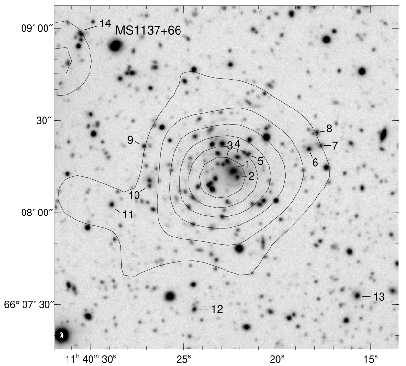
Figure 2: An optical image of the central region of the X-ray cluster MS1137.5+6625, with X-ray emission contours overlaid. The ROSAT HRI image was adaptively smoothed with Gaussians such that the product of the Gaussian widths and the number of counts inside that Gaussian was nearly constant. The contours start three sigma above the background ($5.2\times 10^{-3}$ cts s^-1 arcmin^-2) and increase in linear steps of $1.57\times 10^{-3}$ cts s^-1 arcmin^-2. The maximum contour value displayed is $1.30\times 10^{-2}$ cts s^-1 arcmin^-2. The galaxies are identified according to Table 3.

The ROSAT HRI obtained observations of MS1137.5+6625 on 3 separate occasions for a total of 100,034 seconds (Table 2). The HRI data were filtered to include only PHA bins 1-7. By excluding the higher PHA bins we reduced the background count rate but sacrificed very few source counts. Contours of X-ray emission are overplotted on an optical image of the cluster from Clowe et al. (1998) in Figure 2. We binned the HRI data into 4″ by 4″ bins and fit a two-dimensional model to the X-ray emission by generating an intrinsic model, convolving that model with the HRI point response function, and fitting that to the binned data (see Hughes & Birkinshaw 1998 for a full description of the technique and software). The background count rate in the HRI image near the cluster was $3.59\times 10^{-3}$ counts s^-1 arcmin^-1. The best fit model to the surface brightness was a circular King model ($I\propto[1+(r/r_{c})^{2}]^{-3\beta+1/2}$) with a core radius $r_{c}$ of $0.25\arcmin\pm_{0.10}^{0.20}$ and $\beta=0.70\pm_{0.15}^{0.45}$ (90% confidence for 2 interesting parameters). In Figure 3 we plot the 68%, 90%, and 95% confidence contours for two interesting parameters, $\beta$ and core radius. The slope $\beta$ is not well measured with the HRI data, but it is consistent with that of low redshift clusters of galaxies. We also fit an elliptical King model to the data, but without significant improvement in $\chi^{2}$. This cluster is more compact than many X-ray clusters, with a core radius of only 71$h^{-1}$ kpc ($q_{0}=0.1$) to 61$h^{-1}$ kpc ($q_{0}=0.5$). The best-fit normalization corresponds to a central surface brightness of $0.023$ HRI counts s^-1 arcmin^-2 which is comparable to other high redshift clusters without strong cooling flows. MS0016+16, for example, has a central surface brightness of $0.047$ HRI counts s^-1 arcmin^-2 (Hughes & Birkinshaw 1998). The nominal center of the X-ray emission in MS1137.5+6625 is $11^{h}40^{m}22.0^{s}$, $+66^{\circ}\,08\arcmin\,17\arcsec$ (J2000).

We converted the observed central surface brightness to physical units by assuming 1 HRI count = $3.77\times 10^{-11}$ erg cm^-2. The calibration was derived by using the IRAF/PROS program called hxflux to convert the count rate to an unabsorbed energy flux between the ROSAT band energies of 0.2-2.5 keV, assuming that $kT=5.7$ keV, log $N_{H}=20.0$, $z=0.78$, and abundances of 30% solar. The conversion is not very sensitive to the assumed abundances, varying by only 1-3% when assumed $kT=4.5-7.5$ and $Z_{Fe}=10-30\%$. The central surface brightness is thus $8.6\times 10^{-13}{\rm erg\,s^{-1}\,cm^{-2}\,arcmin^{-2}}$.

We estimated a gas mass for this cluster by converting the central HRI surface brightness into a central electron density of $2.0\pm^{0.6}_{0.5}\times 10^{-2}h^{1/2}$ cm^-3 using the relation of Henry & Henriksen (1986), modified to account for redshift effects on surface brightness (Hughes & Birkinshaw 1998). The gas mass is integrated out to a radius of 0.5 $h^{-1}$ Mpc by assuming $\rho=1.14n_{e}m_{H}[1+(r/r_{c})^{2}]^{-3\beta/2}$, with values of $r_{c}$ and $\beta$ from our fit to the HRI observations. The value 1.14 is the mass per free electron in a fully-ionized, primordial hydrogen/helium plasma in units of the proton mass, $(1.+4A_{He})/(1.+2A_{He})$ where $A_{He}$, the number fraction of He/H is 0.08. The gas mass interior to $0.5\,h^{-1}$ Mpc found in this way is $0.9-1.2\pm^{0.2}_{0.3}\times 10^{13}h^{-5/2}M_{\odot}$, for $q_{0}=0.5$ and $0.1$ respectively. The main uncertainty in the central electron density and the gas mass inside 0.5 h^-1 Mpc arises from our fit to the HRI data. The uncertainties reflect the 90% statistical uncertainties in $\beta$, $r_{c}$, and the appropriate fit normalization.

The total mass interior to $0.5\,h^{-1}$ Mpc can be estimated if we assume that the ICM is nearly isothermal and in hydrostatic equilibrium within the cluster gravitational potential. The total mass inside a radius of $0.5\,h^{-1}$ Mpc would then be $2.1\times 10^{14}\pm^{1.5}_{0.8}h^{-1}M_{\odot}$ (relatively insensitive to $q_{0}$). The main sources of uncertainty are in the $\beta$ value for the gas distribution ($\beta$ is proportional to the total mass under our assumptions) and the absolute temperature. The quoted uncertainty does not reflect the systematic uncertainty in the assumption of hydrostatic equilibrium, which, according to current numerical simulations (e.g., Navarro, Frenk & White 1995; Evrard 1997; Roettiger, Stone & Mushotzky 1997; Roettiger, Burns, & Loken 1996), can be considerable ($\sim 20-50\%$) but less than the statistical uncertainities of our data. The minimum mass estimate from weak lensing in this cluster is $2.45\pm 0.8\times 10^{14}h^{-1}M_{\odot}$ interior to 0.5 $h^{-1}$ Mpc (Clowe et al. 1998), consistent with the X-ray derived mass inside the same radius.

The gas fraction within $0.5\,h^{-1}$ Mpc is therefore $0.02-0.08\,h^{-3/2}$, but this ratio could be as high as $0.10\,h^{-3/2}$ if both $\beta$ and the actual virial temperature are at the low end of their respective 90% uncertainty ranges. Furthermore, according to the simulations mentioned in the previous paragraph, cluster masses derived from X-ray temperatures can exceed their actual masses by up to $20\%$, so the true gas fraction could be up to 20% higher ($f_{g}\sim 0.12\,h^{-3/2}$) if the gravitational mass is overestimated. These observations, therefore, do not necessarily imply that the gas fraction in this cluster is any different from the gas fractions typical of lower-redshift clusters.

In earlier work, Donahue (1996) reported that the cluster MS0451.6-0305 showed evidence for a lower gas fraction than is typical of local clusters. A re-analysis of the HRI data for the cluster MS0451.6-0305 (z=0.54) using the techniques described here give a central surface brightness of $0.029$ HRI counts s^-1 arcmin^-2 and a best-fit $\beta=0.6_{-0.05}^{+0.2}$ and $r_{core}=0.5_{-0.05}^{+0.25}$ arcminutes (90% uncertainties for two interesting parameters.) The corresponding central electron density is $n_{e}=0.012^{+0.001}_{-0.002}h^{1/2}$ cm^-3, and the gas mass inside 0.5 $h^{-1}$ Mpc is $2.4-2.7\pm 0.2\times 10^{13}h^{-5/2}M_{\odot}$, for $q_{0}=0.5$ and $0.1$ respectively. This estimate corrects the value in Donahue (1996) which omitted a $(1+z)^{3/2}$ factor for the central density. The gas fraction for MS0451.6-0305 is thus revised upward to span $0.048-0.096h^{-3/2}$, spanning the 90% ranges of allowed $\beta$, core radius, and $kT=10.9\pm 1.2$ (Donahue 1996; this work). Thus we find no evidence that the gas fraction has changed in cluster cores from either of the clusters MS1137.5+6625 or MS0451.6-0305. (The HRI data for cluster MS1054.4$-$0321 does not allow for straightforward conversion of the measured emissivity to gas mass since the X-ray emission profile shows internal structure and the cluster may not be hydrodynamically relaxed (Donahue et al. 1998).)

The cooling time within the core of MS1137.5+6625, estimated from the ratio $(5kT/2)/(\epsilon_{ff}(T)/n_{e})$, where $\epsilon_{ff}(T)$ is the free-free emissivity of hydrogen gas at temperature $T$, is somewhat shorter than the Hubble time at $z=0.78$. We assumed $\epsilon_{ff}(T)=1.4\times 10^{-27}g_{ff}[1.14n_{e}^{2}]T^{0.5}$ erg cm^-3 s^-1, where $g_{ff}\sim 1.25$, $T$ is the electron temperature in units of Kelvins, $n_{e}$ is the electron density, and the factor 1.14 comes from the assumption that the gas is fully ionized. The cooling rate is estimated by computing the amount of gas inside the radius at which the cooling time equals the Hubble time at the redshift of the cluster, and dividing by the Hubble time at the cluster redshift. For a range of cosmological assumptions ($H_{0}=50-75$ km s^-1 Mpc^-1, $q_{0}=0.0-0.5$), the derived cooling rate lies between 20 and 400 M_⊙ yr^-1, where the slower rates correspond to $q_{0}=0.5$. The cooling rates estimated in this way are far more sensitive to $q_{0}$ than to $H_{0}$. For $H_{0}=75$ km s^-1 Mpc^-1 and $q_{0}=0.1$, the inferred cooling rate is 130 M_⊙ yr^-1.

2.3 Keck-II Observations

Multi-object spectroscopy of galaxies in the cluster MS1137.5+6625 was obtained with LRIS (Oke et al. 1995) on the Keck-II telescope on Feb. 17, 1998. We used a 1.5^′′ slit width and a 300 line/mm grating at 5000 Å, with the GG495 filter. The wavelength scale was 2.47 Å/pix; the spatial scale was 0.215^′′/pixel. The seeing was 0.8^′′ - 1.0^′′. Three masks with total exposure times of 6300, 6900, and 7200 seconds were used to obtain spectra.

Twenty-three galaxies in MS1137.5+6625 have concordant redshifts (Table 3). One galaxy was discarded by the three-sigma clipping code used to compute the velocity dispersion (Danese, De Zotti, & Di Tullio 1980), for 22 cluster members in total. The dispersion for the 22 galaxies is $884\pm^{185}_{124}$ km/sec (1-sigma errors), with a mean redshift of $z=0.7842\pm 0.0003$. A similar result was obtained using ROSTAT (Beers, Flynn & Gebhardt 1990). The velocity dispersion corresponds to a cluster temperature of $kT\sim\mu m_{p}\sigma_{\rm 1D}^{2}=4.8\pm 0.4$ keV (1-sigma errors). Although the velocities of the cluster galaxies may appear to be a little “cooler” than the cluster gas, in fact the temperature and velocity dispersion are statistically in agreement. The temperature and velocity dispersion of MS1137.5+6625 are completely consistent with the observed relationship for lower redshift clusters (Mushotzky & Scharf 1997) and for other $z=0.5-0.8$ EMSS clusters (Donahue et al. 1998). The agreement of the X-ray temperature and the velocity dispersion and the agreement of the X-ray mass and the lensing mass from Clowe et al. (1998) suggest that the cooling flow in this cluster does not affect the emission-weighted temperature significantly.

2.4 Iron Abundance at $z\sim 0.8$

The iron line detection in MS1137.5+6625, if real, is the most distant iron line detected in the EMSS cluster sample. The best-fit abundance is consistent with the abundances of low-redshift clusters; however, the uncertainty range is disappointingly large. In order to improve our constraints on ICM abundances at $z\sim 0.8$, we can combine our ASCA data on MS1137.5+6625 with our existing ASCA data on MS1054.4$-$0321, the other EMSS cluster at this redshift (Donahue et al. 1998).

We estimated a “mean” iron abundance of clusters at $z\sim 0.8$ by simultaneously fitting all of the ASCA data for MS1137.5+6625 and MS1054.4$-$0321. We allowed the temperatures of the two clusters to differ, but required their metal abundances to be equal. The Galactic absorption columns to each cluster and the redshifts were fixed at their individual values. The resulting iron abundance was $Z_{Fe}=0.33\pm^{0.26}_{0.23}$ for a formal 90% confidence range for one interesting fit parameter ($\Delta\chi^{2}=2.70$.)

The mean iron abundance at $z\sim 0.8$ is statistically more significant than the abundance determinations for the individual clusters and is similar to that of clusters of galaxies at lower redshifts. This result implies that the metal enrichment of the cluster ICM, presumably from supernovae erupting in cluster galaxies, must have occurred before $z\sim 0.8$.

3 High Redshift Complete Sample of Clusters of Galaxies

A primary motivation for observing distant clusters with ASCA has been to establish a temperature function for high-redshift clusters that can be compared with cosmological models. Now that we have ASCA data in hand for almost all the EMSS clusters at $z>0.5$, we can construct a high-redshift temperature function that is based on a complete sample of clusters (Table 4). The flux limit of our subsample of the EMSS, set by ASCA’s capabilities, is approximately $1.80\times 10^{-13}\,{\rm erg\,s^{-1}\,cm^{-2}}$ in the EMSS detection cell of $2.4\times 2.4$ arcminutes, within the Einstein bandpass of 0.3-3.5 keV. Some of the original clusters listed in Henry et al. (1992) are revised in our updated sample. We have revised the redshift of cluster MS1241.5+1710 upward from 0.31 to 0.54, based on spectroscopy of the cD galaxy and one other galaxy. The cluster candidate MS2053.7-0449 at $z=0.58$ drops out of the sample because short followup observations by the ROSAT HRI failed to detect it. Its X-ray flux is thus likely to be below the flux limits of our sample. However, it was definitely detected by the Einstein IPC, and long ROSAT HRI and ASCA observations have been made (PI: Henry). The cluster candidate MS1610.4+6616 (Gioia & Luppino 1994) is an X-ray point source and is excluded from our sample, since it is a likely AGN.

The resulting EMSS sample of clusters of galaxies with redshifts greater than 0.5 is listed in Table 4. The X-ray temperatures for the cluster MS 1241.5+1710 were extracted and fit from archival ASCA data using the same procedure as described above. We also analyzed the complete suite of ASCA data for the MS0015.9+1609 cluster, excluding the SIS0 and SIS1 dataset of the second observation contained in the HEASARC because they exhibited severe anomalies. This analysis differs somewhat from the Hughes & Birkinshaw (1998) analysis in that our analysis included 6 out of the 8 ASCA datasets available as well as the ROSAT PSPC data, while Hughes & Birkinshaw (1998) analyzed the PSPC data and the GIS data from the Performance Verification stage of the ASCA mission only. However, the mean temperature that we obtain ($8.7^{+1.8}_{-0.6}$ keV, 90% confidence limits) is statistically consistent with their temperature limits of $7.55^{+0.72}_{-0.58}$ keV ($1-\sigma$ errors), and all other best fit spectral values (Fe/H and $N_{H}$) are nearly identical. These fits are also consistent with the results of Furuzawa et al. (1998) who obtain a best fit temperature of $8.0\pm^{1.0}_{0.8}$ keV. The detection cell fluxes (Table 4) are from the Einstein IPC (0.3-3.5 keV). The total fluxes within a 5-6 arcmin aperture were measured from the ASCA GIS3 observations of each cluster. (The SIS observations do not in general provide a good estimate of the total flux because flux is lost off the side of the main CCD or between the CCDs.) Luminosities were computed within XSPEC (Arnaud 1996), assuming the appropriate cosmological models. We could recover, to within uncertainties, estimates of the Einstein detect cell flux from the large aperture ASCA GIS fluxes and estimates about the cluster structure (see Table 4). From the GIS total fluxes, we determined the bolometric X-ray luminosity for each cluster (by using the dummyrsp capability in XSPEC). The original Einstein detection fluxes were used to compute maximum volume $V_{\rm max}$ within which the X-ray emission from the cluster would exceed the flux limits of the EMSS, assuming that all clusters have an average core radius of $0.125h^{-1}$ Mpc (Table 4).

We derived maximum volumes for each of the clusters following the prescription of Henry et al. (1992), using the Einstein detection cell fluxes and assuming a mean core radius of $125h^{-1}$ kpc and $\beta=2/3$. The assumed source parameters did not influence the maximum volumes significantly, so we simply assumed the same parameters for all of the clusters. For most of the clusters, the maximum volume spanned the redshift limits of the sample ($0.5\leq z\leq 0.9$). The cumulative temperature function was then computed by summing $1/V_{\rm max}$ for each $T\geq T_{i}$.

The temperature function for these high-$z$ clusters differs only modestly from the temperature functions for lower-redshift clusters. Figure 5 shows the temperature functions for clusters at $z=0.04-0.09$ clusters (data from Markevitch 1998), $z=0.3-0.4$ (Henry 1997), and $z=0.5-0.9$ (this paper) for a $q_{0}=0.5$ cosmology. The statistical review of these data and comparison to semi-analytic models are continued in our analysis paper (Donahue & Voit 1999), which finds that this amount of evolution in the temperature function is consistent with $\Omega_{M}=0.45\pm 0.1$ (open universe) or $\Omega_{M}=0.27\pm 0.1$ (flat universe), with systematic uncertainties of an additional $\pm 0.1$ (see also Donahue 1999 for our preliminary report of this work). As we reported in Donahue et al. (1998), the presence of hot clusters ($>8\,{\rm keV}$) at $z>0.5$ in the EMSS strongly suggests that $\Omega_{M}<1$.

4 Bolometric Luminosity-Temperature Evolution

The relationship between the cluster X-ray luminosity and the mean temperature of its ICM and the evolution of that relationship are relevant both for what we can learn about cluster ICM physics and for tests of cosmology from studying the evolution of the cluster luminosity function.

At low redshift, the X-ray luminosities of galaxy clusters are related to their temperatures via a power law: $L_{x}\propto T_{x}^{\alpha}$ with $\alpha\sim 3$ (Edge & Stewart 1991; David et al. 1993, Arnaud & Evrard 1998). Not all clusters are isothermal and the scatter in this relation can be reduced if one corrects for the cooler gas often found in cluster cores. Recent relations derived by excluding the cool regions (Markevitch 1998) or by accounting for them with models (Allen & Fabian 1998) arrive at somewhat flatter power-law slopes. All the cluster temperatures and luminosities in our high-$z$ EMSS sample are consistent with these low-$z$ temperature-luminosity relations. Here we assess the significance of that consistency.

The scaling of cluster luminosities with cluster temperatures presumably depends on the thermal history of the ICM. In general, the luminosity of a cluster should scale with the core density ($n_{c}$), the core radius ($r_{c}$), and the temperature: $L_{X}\propto n_{c}^{2}r_{c}^{3}T^{1/2}$. According to self-similar models of cluster formation in a critical universe, the cluster temperature should scale as $T_{X}\propto n_{c}r_{c}^{2}$, and given $n_{c}\propto(1+z)^{3}$, one finds $L_{X}\propto(1+z)^{3/2}T^{2}$ (Kaiser 1986). The power-law dependence of $L_{X}$ on $T_{X}$ in this relation is somewhat shallower than observed. One way to account for this discrepancy is to suppose that the ICM of each cluster undergoes a similar pre-heating event that fixes the minimum specific entropy at a value common to all (Kaiser 1991; Evrard & Henry 1991). Then the core density is determined by the ICM temperature ($n_{c}\propto T^{3/2}$ for an ideal gas), and the luminosity should scale as $L_{X}\propto T_{X}^{11/4}$, with redshift evolution depending on how and when the cluster gas heats or cools (e.g., Bower 1997).

Furthermore, the scaling of cluster luminosities with cluster temperatures is an important step in the exercise of connecting the observed X-ray luminosity function of clusters at different redshifts with predictions of the evolution of the cluster mass function. If the evolution of the cluster $L_{X}-T_{X}$ relation is strongly positive ($L_{x}\propto T_{x}^{3}(1+z)^{A}$, where $A\sim 2$), then the lack of evolution in the cluster luminosity function, at least at $L_{x}<3\times 10^{44}~{}{\rm erg\,s^{-1}}$ (Rosati et al. 1998; Ebeling et al. 1998; Sadat, Blanchard, & Oukbir 1998; Mathiesen & Evrard 1998), is remotely consistent with the strong evolution of the mass function predicted by $\Omega_{M}=1$ models (Borgani et al. 1999). This consistency arises because the evolution in the mass function may be counteracted by evolution in the $L_{X}-T_{X}$ relation (see also Oukbir & Blanchard 1992 for the EMSS sample).

In order to constrain the redshift evolution of the $L_{X}$–$T_{X}$ relation with observations, we have compiled data on $z>0.1$ cluster bolometric luminosities, temperatures, and redshifts from Mushotzky & Scharf (1997), Donahue (1996), Donahue et al. (1998), and Henry (1997). We have added cluster AX2019 (Hattori et al. 1997) to this sample and have revised the redshift, luminosity, and temperature of the cluster MS1241.5+1710 as described above.

Since we cannot correct our high-redshift temperatures for deviations from isothermality with our current data, we have chosen to compare mean temperatures of clusters at low redshift with mean temperatures of clusters at high redshift and to quantify the higher intrinsic dispersion incurred. For simplicity, we compare the data with an $L_{X}$–$T_{X}$ relation assuming a power-law redshift dependence: $L_{x}\propto T_{x}^{\alpha}(1+z)^{A}$ (Borgani et al. 1999). Formally, the observational uncertainties in the temperature measurements are often significantly smaller than the scatter in the relation, demonstrating that there are physical effects that are not taken into account by a simple relation, such as cooling flows (see Allen & Fabian (1998); Markevitch (1998) for how these effects might be handled in X-ray data with sufficient resolution and signal to noise.)

For illustrative purposes, we plot the $z=0.3-0.5$ and the $z=0.5-0.9$ bolometric luminosity and temperature data in Figure 6, along with the Markevitch bolometric $L_{x}-T_{x}$ fit to the relation, with $1\sigma$ dispersion to corrected temperatures and luminosities of low-redshift clusters ($L_{x}=3.11\times 10^{44}h^{-2}{\rm erg\,s^{-1}}T_{6}^{2.64}$ where $\sigma_{log~{}L}=0.103$). We note that the uncorrected high-redshift points cluster around the low-redshift relation within the dispersion. In Figure 6, the normalization of the low-redshift Markevitch relation has been evolved appropriate to $A=2$ for two epochs, $z=0.3$ and $z=0.8$. This amount of evolution is ruled out by the data.

To test the significance to which evolution of the $L_{x}-T_{x}$ relation could be constrained, the procedure was to obtain a linear regression fit of the expression $\log T_{\rm fit}=\log T_{0}+(1/\alpha)\log L_{x}-(A/\alpha)\log(1+z)$ to the redshift, luminosity, and temperature data. We weighted each point by defining an effective standard deviation $\sigma_{\rm eff}=0.6(T_{h}-T_{l})/2$, where $T_{h}$ and $T_{l}$ are the upper and lower bounds on the 90% confidence interval of the temperature. This value for $\sigma_{\rm eff}$ roughly reproduces the width of the 68% confidence interval normally associated with $1\sigma$. The David et al. (1993) cluster temperature catalog provides both 68% and 90% confidence limits. The mean ratio between the 68% intervals and the corresponding 90% intervals is $0.60\pm 0.06$ for $kT>6$ keV.

To check this estimate, the actual probability distributions for each of the measurements were derived for the 5 EMSS clusters in our highest redshift sample. We then fit the probability distributions to Gaussians. The results of this exercise demonstrated that the estimate of the size of the 68% uncertainties from the 90% uncertainties as obtained from the literature is reasonable. However, we also note in the cases where the error bars are uneven in size (the upper error bar is larger than the lower error bar), the mean temperature from the Gaussian fit is higher than the actual best-fit temperature, and the errors from the Gaussian fit are approximately the mean of the two original errors (Table 5.)

Formally, the best fitting $L_{x}-T_{x}$ relation is not a good fit, owing to the significant intrinsic scatter in the relationship between luminosity and temperature. Intrinsic scatter can be caused by inclusion of “cooling-flow” emission from the core of the galaxy and other processes that affect the luminosity of the cluster, which is very sensitive to the electron density in the ICM. To ensure that our $\chi^{2}$ values reflected the actual scatter in the $L_{x}-T_{x}$ relation, we added a constant intrinsic scatter term to each measurement’s standard deviation in quadrature, so that the reduced $\chi^{2}=1$ for the best fit. In this case, the intrinsic scatter of the $L-T$ relationship in the temperature of clusters with $kT>3$ keV and $z=0.1-0.9$ is $\sim 0.08$ in units of log keV. The intrinsic scatter in log T for these clusters is nearly identical to that of low redshift clusters. Markevitch (1998) finds an intrinsic scatter of $\sigma_{{\rm log~{}}T}\sim 0.09$ for uncorrected temperature data. Mushotzky & Scharf (1997) also noted that the intrinsic variance in the $L-T$ did not change with redshift in their analysis of a subset of the clusters analyzed here, with $z=0.14-0.55$.

Because the observed luminosities of clusters at these moderate redshifts depend on the assumed cosmology, we fit the $L_{X}$–$T_{X}$ relation for three different cosmologies. Our results for the best fit $A$ vs. $\Delta\chi^{2}$ are displayed in Figure 7. The most relevant cosmology for $\Omega_{M}=1$ models is the flat $q_{0}=0.5$ assumption. The $\Delta\chi^{2}$ distribution for $A$ in a critical ($q_{0}=0.5$) cosmology, shown in Figure 7, demonstrates that self-similar evolution ($A=1.5$) is a poor fit to the data, even when intrinsic dispersion is accounted for. The best-fit value of $A$ is actually slightly negative and $\Delta\chi^{2}=9.5$ for $A=1.5$. Our results are statistically consistent with those obtained by Reichart, Castander, & Nichol (1999), who assumed all of the EMSS clusters had a cluster temperature of 6 keV and who fit only the $z\leq 0.5$ clusters.

The absence of $L_{X}$–$T_{X}$ evolution in our sample poses serious difficulties for cluster evolution in a critical universe. The reason for this difficulty is that in order to account for the lack of evolution observed in the cluster luminosity function out to $z\sim 0.8$ (Rosati et al. 1998), models in which $\Omega_{M}=1$ must include sufficient luminosity evolution to mask the dramatic number evolution in the mass function that occurs if $\Omega_{M}=1$ (Viana & Liddle 1996; Eke, Cole & Frenk 1996). The power-law index of $A\approx 2-3$ which reproduces the lack of evolution of the observed cluster luminosity function at the outer limits of statistical and systematic uncertainties (Borgani et al. 1999) results in an extremely poor fit to our high redshift $L_{X}$–$T_{X}$ data for any $q_{0}$.

5 Conclusions

We have presented X-ray observations from the ASCA and ROSAT satellites, and new Keck-II galaxy redshifts for the EMSS cluster MS1137.5+6625 at $z=0.78$. This cluster is the last cluster in our complete sample of high-redshift EMSS clusters of galaxies to be observed with ASCA. X-ray spectra from ASCA constrain the temperature of the intracluster plasma to be $kT=$  $5.7^{+2.1}_{-1.1}$  keV. The total X-ray luminosity within a 5^′ radius GIS aperture is $1.9-2.8\times 10^{44}\,h^{-2}$ erg s^-1 in the 2-10 keV band in the rest frame of the cluster ($q_{0}=0.0-0.5$). The luminosity and temperature are consistent with the empirical relation between X-ray luminosity and redshift for low-redshift clusters of galaxies.

The velocity dispersion of 22 member galaxies measured with the Keck-II telescope and LRIS is $884\pm^{185}_{124}$ km/sec, which is consistent with the value of the ICM temperature. This consistency implies that the thermal properties of the X-ray gas and the dynamics of the galaxies are both governed by the gravitational potential of the cluster. Clowe et al. (1998) report a weak lensing mass of $2.45\pm 0.8\times 10^{14}\,h^{-1}\,M_{\odot}$ interior to 0.5 h^-1 Mpc. This is consistent with the isothermal mass estimated from the cluster temperature and the best-fit $\beta=0.7$ from the HRI observations of $2.1\times 10^{14}\,h^{-1}\,M_{\odot}$. Therefore the cluster temperature, the galaxy velocity dispersion, and the weak lensing mass, all independent measures of the cluster gravitational mass, are all self-consistent at a radius of 0.5 $h^{-1}$ Mpc.

We report a mean iron abundance for $z\sim 0.8$ clusters of galaxies that is consistent with that of low redshift clusters of galaxies by simultaneously fitting all of the ASCA spectra for MS1054.4$-$0321 and MS1137.5+6625. The mean abundance is $0.33$ solar with a formal one-dimensional 90% uncertainty range of 0.10–0.59. This measurement is one of the highest-redshift detections of intracluster iron.

We have estimated a gas fraction that is consistent with being the same as that of clusters at low redshift. Our main uncertainties are primarily in constraining the gas distribution of the cluster and secondarily in constraining the cluster temperature. The cluster may have a modest cooling flow of $\sim 20-400$ M_⊙ yr^-1. In summary, the velocity dispersion, temperature, gas fraction, and iron abundance of MS1137.5+6625 are all similar to those properties in lower redshift clusters of similar luminosity.

The X-ray luminosity-temperature relation for clusters appears to evolve little out to $z\sim 0.8$. We supplemented the Mushotzky & Scharf (1997) $L_{x}-T_{x}$ dataset with the two $z=0.8$ EMSS clusters, MS1054.4$-$0321 and MS1137.5+6625, the $z=0.9$ cluster discovered by Hattori et al. (1997), the Henry $z=0.3-0.4$ clusters, and one of the Henry clusters revised to a higher redshift in order to constrain the parameter $A$, where $L_{x}\propto T_{x}^{\alpha}(1+z)^{A}$. We exclude $A=3/2$ at greater than $3\sigma$ confidence for $q_{0}=0.5$. Values of $A=2-3$, required to explain why the X-ray luminosity function does not appear to change out to $z\sim 0.8$ if $\Omega_{m}=1$, are strongly ruled out by this data.

We present a cluster temperature function for $z=0.5-0.9$ based on a complete sample of 5 EMSS clusters. A companion paper (Donahue & Voit 1999) compares this high-redshift temperature function to cosmological models which predict how the cluster temperature function should evolve.

Figure 1: Binned, background-subtracted ASCA spectra and the best-fit thermal model. For clarity of display only, the individual SIS and GIS X-ray spectra and corresponding models were averaged to produce this figure.

Figure 3: Contour plot for the two-dimensional uncertainties for $\beta$ and core radius for MS1137, where $\Delta\chi^{2}=2.30$, 4.61, and 6.17 corresponding to 68%, 90% and 95% confidence intervals.

Figure 4: We plot the result of a simultaneous fit of two $z=0.8$ cluster iron abundances. We allowed the fluxes and the temperatures of the two clusters to be different but forced the iron abundance to be the same. We plot the two-dimensional $\chi^{2}$ contours at 68.3%, 90% and 99% confidence levels ($\Delta\chi^{2}=2.30$, 4.61 and 9.21) for two interesting parameters for the mean cluster iron abundance in units of the solar abundance and temperature of MS1137.5+6625 in keV.

Figure 5: The temperature function at three different redshift ranges from $z=0.04-0.09$ (data from Markevitch 1998) in solid line, $z=0.3-0.4$ (Henry 1997, sample revised as discussed in the text), dotted line, and $z=0.5-0.9$ (this paper) for $q_{0}=0.5$ in the dashed line. The temperature function changes slightly from one redshift range to the next. $N(\geq T)$ is in the units of number of clusters per cubic Mpc (Mpc${}^{-3}h^{3}$) and temperature is plotted in keV. The evolution in the temperature function is consistent with $\Omega=0.3-0.45$ (Donahue & Voit 1999.)

Figure 6: Bolometric luminosities and temperatures for $z>0.3$ EMSS clusters and other clusters from the literature are plotted here. The filled circles are clusters with $z=0.5-0.9$, and the open diamonds are clusters with $z=0.3-0.5$. The solid lines indicate the low-redshift bolometric luminosity temperature relation from Markevitch (1998) where $L_{x}\propto T_{x}^{2.64}$, and a dispersion in log $L_{x}$ of 0.103. The luminosities in this plot were computed assuming $q_{0}=0.5$. The dotted and dashed lines indicate where the low-redshift relation evolves if $A=2$ and $z=0.3$ and $z=0.8$ respectively. Note that the Markevitch relation is for clusters whose central cooler regions have been removed from the data, while the $z>0.3$ data are uncorrected. Corrected cluster temperatures would tend to move to the right in this plot. The two most serious outliers are $z\sim 0.4$ clusters from the Mushotzky & Scharf (1997) sample, RXJ1347.5-1145 ($kT\sim 11.4$ keV) and MS2137.3-2353 ($kT\sim 4.4$ keV). They are both massive cooling flow clusters with unusually high luminosities for their temperatures (Allen & Fabian 1998).

Figure 7: The change in $\chi^{2}$ for a fit to a single interesting parameter, $A$, in which the luminosities and temperatures of a sample of moderate redshift ($z=0.1-0.9$) clusters is fit to the relation $L_{x}\propto T_{x}^{\alpha}(1+z)^{A}$, including an intrinsic dispersion. (See text for details.) Luminosities were computed assuming $q_{0}=0.5$ (solid line), $q_{0}=0.15$ (dashed line), and a flat universe where $\Omega_{m}=0.3$ and $\Lambda=0.7$ (dot-dash line). One, two and three sigma levels are marked horizontally across the plot. A model where $A=3/2$ is ruled out at $>3$ sigma for the $q_{0}=0.5$.

Table 1: ASCA Observations

Detector	Good Exposure	Count Rate
	(seconds)	($10^{-3}$ cts/s)
SIS0	71,377	$6.7\pm 0.4$
SIS1	70,528	$4.5\pm 0.3$
GIS2-spectrum	66,432	$3.7\pm 0.4$
GIS3-spectrum	66,494	$4.4\pm 0.4$
GIS2-5 arcmin	66,432	$4.5\pm 0.6$
GIS3-5 arcmin	66,494	$6.1\pm 0.7$

Table 2: HRI Observations

Dataset ID	Observation Dates	Exposure Time
RH800662N00	May 19-25, 1995	3,563 seconds
RH800784N00	Oct 12-Dec 4, 1995	32,202 seconds
RH800784A01	May 6-30, 1996	64,269 seconds

Table 3: Redshift Catalog for MS1137.5+6625

RA (J2000)	DEC (J2000)	ID	Redshift
11 40 22.3	+66 08 15	1	$0.7844\pm 0.0010$
11 40 22.0	+66 08 12	2	$0.7903$
11 40 22.6	+66 08 17	3	$0.7844\pm 0.0006$
11 40 22.0	+66 08 19	4	$0.7927\pm 0.0007$
11 40 21.4	+66 08 20	5	$0.7826\pm 0.0009$
11 40 17.7	+66 08 23	6	$0.7808$
11 40 16.9	+66 08 25	7	$0.7909\pm 0.0007$
11 40 17.2	+66 08 29	8	$0.7916\pm 0.0007$
11 40 27.4	+66 08 23	9	$0.7761\pm 0.0011$
11 40 27.0	+66 08 09	10	$0.7760\pm 0.0015$
11 40 29.3	+66 08 02	11	$0.7831\pm 0.0001$
11 40 24.5	+66 07 26	12	$0.7823\pm 0.0013$
11 40 14.8	+66 07 32	13	$0.7824\pm 0.0009$
11 40 30.8	+66 09 03	14	$0.7900\pm 0.0011$
11 40 15.1	+66 09 22	15	$0.7773\pm 0.0008$
11 40 17.4	+66 09 14	16	$0.7909\pm 0.0011$
11 40 42.8	+66 10 19	17	$0.7814\pm 0.0010$
11 40 40.4	+66 07 52	18	$0.7889\pm 0.0003$
11 40 37.1	+66 07 25	19	$0.7902$
11 40 10.3	+66 07 18	20	$0.7898\pm 0.0008$
11 40 05.9	+66 08 05	21	$0.7790$
11 39 58.9	+66 08 00	22	$0.7792\pm 0.0007$
11 40 06.0	+66 08 18	23	$0.7714$

Table 4: Summary of EMSS Cluster X-ray Parameters

Cluster	MS0451-03	MS1241+17	MS0015+16	MS1137+66	MS1054-03
Redshift	0.539	0.540	0.5455	0.785	0.828
kT (keV)	$10.9\pm 1.2$	$6.4\pm^{1.8}_{1.1}$	$9.9\pm^{1.1}_{1.0}$	$5.7^{+2.1}_{-1.1}$	$12.3\pm^{3.7}_{2.1}$
GIS aperture (arcmin)	6.0	5.0	6.0	5.0	5.0
$F_{x}$ (GIS, 0.3-3.5 keV obs)	$19.0\pm 0.4$	$7.1\pm 0.4$	$21.0\pm 0.4$	$2.7\pm 0.3$	$5.6\pm 0.3$
$F_{x}$ (GIS, 2-10 keV obs)	$22.0\pm 0.5$	$6.2\pm 0.3$	$23.0\pm 0.4$	$1.8\pm 0.2$	$6.1\pm 0.3$
$L_{44}$ (2-10 keV rest)	$10.6\pm 0.2$	$3.4\pm 0.2$	$12.0\pm 0.2$	$2.8\pm 0.3$	$8.4\pm 0.5$
$L_{44}$ (bolometric)	$21.0\pm 0.4$	$6.1\pm 0.3$	$22.0\pm 0.4$	$4.8\pm 0.5$	$16.6\pm 0.9$
$F_{x,det}$ (Einstein, 0.3-3.5 keV)	$9.54\pm 1.71$	$4.23\pm 1.08$	$7.06\pm 0.79$	$1.89\pm 0.36$	$2.11\pm 0.25$
$F_{x,det}$ (GIS, 0.3-3.5 keV)	$12.4\pm 1.2$	$4.31\pm 0.5$	$12.8\pm 0.3$	$2.46\pm 0.3$	$2.19\pm 0.25$
core radius (arcmin)	0.5	0.68	0.74	0.25	0.9
Vol, $q_{0}=0.5$	15.58	4.24	11.60	4.45	6.25
Vol, $q_{0}=0.15$	21.97	5.73	16.26	6.77	9.67
Vol, $\Omega_{M}=0.3$,$\Lambda=0.7$	34.12	8.59	25.91	10.78	15.55

Table 5: Comparison of Actual Fit Temperatures and 1-$\sigma$ Errors to Mean Fit Temperatures

Cluster	Actual Fit	Mean Fit from Gaussian
	(keV), 1-sigma	(keV), 1-sigma
MS1054	$12.3^{+1.9}_{-1.3}$	$12.6\pm 1.6$
MS1137	$5.8^{+0.9}_{-0.7}$	$6.0\pm 0.9$
MS0451	$11.0^{+0.9}_{-0.8}$	$11.1\pm 0.9$
MS0016	$9.9^{+0.7}_{-0.6}$	$9.9\pm 0.6$
MS1241	$6.4^{+0.8}_{-0.7}$	$6.5\pm 0.8$

References

- (1) Allen, S. W. & Fabian, A. C. 1998, MNRAS, 297, L57.
- (2) Anders, E. & Grevesse, N. 1989, Geochmica et Cosmochimica Acta 53, 197.
- (3)
- (4) Arnaud, K. A. 1996, Astronomical Data Analysis Software and Systems V, eds. G. Jacoby and J. Barnes, ASP Conf. Series vol 101.
- (5)
- (6) Arnaud, M. & Evrard, A. E. 1998, MNRAS, submitted (astro-ph/9806353).
- (7)
- (8) Bahcall, N. A., Fan, X., Cen, R. 1997, ApJ, 485, L53.
- (9) Bahcall, N. A. & Fan, X. 1998, ApJ, 504, 1.
- (10)
- (11) Beers, T.C., Flynn, K., & Gebhardt, K. 1990, AJ, 100, 32.
- (12)
- (13) Borgani, S., Rosati, P., Tozzi, P., Norman, C. 1999, ApJ, in press, May 20.
- (14)
- (15) Bower, R. G. 1997, MNRAS, 288, 355
- (16)
- (17) Carlberg, R. G., Yee, H. K. C., Ellingson, E., Abraham, R., Gravel, P., Morris, S., & Pritchet, C. J. 1996, ApJ, 462, 32
- (18)
- (19) Clowe, D., Luppino, G. A., Kaiser, N., Henry, J. P., Gioia, I. M., 1998, ApJ, 497, L61.
- (20)
- (21) Danese, L., De Zotti, G. & Di Tullio, G. 1980, å, 82, 322.
- (22)
- (23) David, L. P., Slyz, A., Jones, C., Forman, W., Vrtilek, S. D., & Arnaud, K. A. 1993, ApJ, 412, 479.
- (24)
- (25) Day, C., Arnaud, K., Ebisawa, K., Gotthelf, E., Ingham, J., Mukai, K., & White, N. 1995, “The ABC Guide to ASCA Data Reduction, Fourth Version”, available by request from the ASCA GOF.
- (26)
- (27) Donahue, M. 1996, ApJ, 468, 79.
- (28) Donahue, M. 1999, in “Observational Cosmology: Development of Galaxy Systems”, PASP proceedings, ed. by Giuricin, G., Mezzetti, M., & Salucci, P.
- (29)
- (30) Donahue, M., Voit, G. M., Gioia, I. M., Luppino, G., Hughes, J. P., Stocke, J. T. 1998, ApJ, 502, 550 (D98).
- (31)
- (32) Donahue, M. & Voit, G. M., 1999, ApJ, submitted.
- (33)
- (34) Ebeling, H., et al. 1998, MNRAS, 301, 881.
- (35)
- (36) Edge, A. C. & Stewart, G. C. 1991, MNRAS, 252, 428.
- (37)
- (38) Eke, V. R., Cole, S., & Frenk, C. S. 1996, MNRAS, 282, 263.
- (39) Eke, V. R., Cole, S., Frenk, C. S., & Henry, J. P. 1998, MNRAS, 298, 1145.
- (40)
- (41) Evrard, A. E. & Henry, J. P. 1991, ApJ, 383, 95.
- (42) Evrard, A. E. 1997, MNRAS, 292, 289.
- (43)
- (44) Furuzawa, A., Yamashita, K., Tawara, Y., Tanaka, Y., & Sonobe, T. 1994, in New Horizon of X-ray Astronomy, eds. F. Makino and T. Ohashi, (Universal Academy Press: Tokyo), p. 541.
- (45)
- (46) Furuzawa, A., et al., 1998, ApJ, 504, 35.
- (47)
- (48) Gioia, I. M., Maccacaro, T., Schild, R. E., Wolter, A., Stocke, J. T. 1990, ApJS, 72, 567.
- (49)
- (50) Gioia, I. M. & Luppino, G. A. 1994, ApJS, 94, 583.
- (51)
- (52) Hattori, M. et al. , 1997, Nature, 388, 146.
- (53)
- (54) Henry, J. P., Gioia, I. M., Maccacaro, T., Morris, S. L., Stocke, J. T. 1992, ApJ, 386, 408. (H92).
- (55)
- (56) Henry, J. P. & Henriksen, M. 1986, ApJ, 301, 689
- (57)
- (58) Henry, J. P. 1997, ApJ, 489, L1
- (59)
- (60) Hughes, J. P., & Birkinshaw, M. 1998, ApJ, 501, 1
- (61)
- (62) Jones, L. R., Scharf, C., Ebeling, H., Perlman, E., Wegner, G., Malkan, M., & Horner, D. 1998, ApJ, 495, 100.
- (63) Kaiser, N. 1986, MNRAS, 222, 323.
- (64) Kaiser, N. 1991, ApJ, 383, 104.
- (65) Luppino, G. A. & Gioia, I. M. 1995, ApJ, 445, L77.
- (66) Luppino, G. A. & Kaiser, N. 1997, ApJ, 475, 20.
- (67)
- (68) Markevitch, M., 1998, ApJ, 504, 27.
- (69)
- (70) Mathiesen, B. & Evrard, A. E. 1998, MNRAS, 295, 769
- (71)
- (72) Mushotzky, R. & Scharf, C. A. 1997, ApJ, 482, L13.
- (73)
- (74) Navarro, J. F., Frenk, C. S., White, S. D. M. 1995, MNRAS, 275, 720.
- (75)
- (76) Oke, J. B. et al. , 1995, PASP, 107, 375.
- (77)
- (78) Oukbir, J. & Blanchard, A. 1992, A&A, 262, L21.
- (79) Reichart, D. E., Castander, F. J., Nichol, R. C. 1999, ApJ, in press.
- (80) Renzini, A., Ciotti, L., D’Ercole, A., Pellegrini, S. 1993, ApJ, 419, 52.
- (81)
- (82) Roettiger, K., Burns, J. O., & Loken, C. 1996, ApJ, 473, 651.
- (83) Roettiger, K., Stone, J. M., Mushotzky, R. F. 1997, ApJ, 482, 588.
- (84)
- (85) Rosati, P., Della Ceca, R., Norman, C., Giacconi, R. 1998, ApJ, 492, L21.
- (86)
- (87) Sadat, R., Blanchard, A., Oukbir, J. 1998, A&A, 329, 21.
- (88)
- (89) Viana, P. T. P. & Liddle, A. R. 1996, MNRAS, 281, 323.
- (90) Vikhlinin, A., McNamara, B. R., Forman, W., Jones, C., Quintana, H. 1998, ApJ, 502, 558.
- (91)
- (92) Yamashita, K. 1994, in New Horizon of X-ray Astronomy, eds. F. Makino and T. Ohashi, (Universal Academy Press: Tokyo), p. 279.
- (93)